Abstract
As artificial intelligence technology progresses, deep learning models are increasingly utilized for machine fault classification. However, a significant drawback of current state-of-the-art models is their high computational complexity, rendering them unsuitable for deployment in portable devices. This paper presents a compact fault diagnosis model that integrates a self-attention SqueezeNet architecture with a hybrid texture representation technique utilizing empirical mode decomposition (EMD) and a gammatone spectrogram (GS) filter. In the model, the dominant signal is first isolated from the audio fault signals by discarding lower intrinsic mode functions (IMFs) from EMD, and subsequently, the dominant signals are transformed into 2D texture maps using the GS filter. These generated texture maps feed as input into the modified self-attention SqueezeNet classifier, featuring reduced model width and depth, for training and validation. Different attention modules were tested in the paper, including the self-attention, channel attention, spatial attention, and convolutional block attention module (CBAM). The models were tested on the MIMII and ToyADMOS datasets. The experimental results demonstrated that the self-attention mechanism with SqueezeNet achieved an accuracy of 97% on the previously unseen MIMII and ToyADMOS datasets. Furthermore, the proposed model outperformed the SqueezeNet attention model with other attention mechanisms and state-of-the-art deep architectures, exhibiting a higher precision, recall, and F1-score. Lastly, t-SNE is applied to visualize the features of the self-attention SqueezeNet for different fault classes of both MIMII and ToyADMOS.
1. Introduction
The modern economy mostly relies on industrial production. The production efficiency mostly depends on the status of the machines. An untimely equipment breakdown leads businesses to a situation in which there is no movement or activity at all. In addition, the repair time of faulty machines causes a negative impact on industrial production. With the advancement of artificial intelligence (AI), researchers have applied AI in machine fault diagnosis to deal with detection and prediction without human intervention []. These AI models are data-hungry, and different sensors [,], including acoustic, vibration, current, voltage, audio, and thermal sensors, are used to collect the machine’s environmental data.
The sensor’s data are in the time domain and one-dimensional. In traditional supervised machine learning models [,], extracted time and frequency domain features are utilized to train and test the support vector machine (SVM), logistic regression (LR), K-nearest neighbors (KNN), random forest (RF), and MLP neural networks (NNs). The advantage of machine learning (ML) models is that the model performance mostly depends on the characteristics of the training dataset, such as quality, quantity, and representation. Feature engineering deals with feature extraction and optimal feature selection. The main limitation of ML models is that they perform well on training datasets. Still, they show poor results for unknown datasets. As the industrial environment and machine faults are not always known, ML models are not suitable due to their feature dependency.
Like other applications, deep learning (DL)-based fault diagnosis is becoming a key issue due to its automatic feature extraction mechanism. The DL architecture consists of several sequential layers, where the output of the first layer will be the output of the second layer, and so on. The final layer is the dense or the output layer. The prior flattened layer converts the output of the convolutional layer into a single 1D vector to feed it as an input into the dense layer and then makes the decision based on the input 1D vector using an activation function. The models use 1D time domain sensor signals for training, validation, and testing [,] and automatically extract the deep features from the sensor data. The attention mechanism helps the model to focus on the most relevant parts or effective information of the input for prediction and classification []. Several attention mechanisms are applied in deep learning architectures, such as the Convolutional Block Attention Module (CBAM) [], the Global Attention Block (GAB) [], the Split-Attention module [], the spatial/channel-wise attention block [], and the Multipath Residual Attention Block (MRAB) [].
In [], Huang et al. show that a 2D-Convolutional Neural Network (CNN) can more accurately extract detailed information than a 1D CNN for time-varying signals by exhibiting a higher accuracy. As a consequence, several researchers have converted 1D sensor data into 2D images for utilizing 2D deep architectures. Islam et al. [] generated a wavelet packet transform-based DDRgram for 1D acoustic emission (AE) signals. Instead of using 1D raw AE signals, they utilized DDRgram (1024 pixels) as an input in an adaptive deep CNN (ADCNN). The experimental results show that the DDRgram-based deep learning model with a small length outperforms the raw 1D signals by requiring less processing time in CPU/GPU architectures.
Shao et al. [] used a pre-trained VGG16 network with ‘ImageNet’ (https://www.image-net.org/, accessed on 3 July 2024) weights to extract the lower-level features and fine-tuned the model with the generated fault images by applying wavelet transform. In [], Wen et al. utilize a pre-trained VGG19 architecture with ‘ImageNet’ and fine-tune it with generated 224 × 224 RGB images by segmenting the 1D CWRU bearing dataset. A summary of the results of the pre-trained state-of-the-art deep learning architectures including ResNet50, InceptionV3, MobileNetv2, Xception, DenseNet121/169/201, and NASNets are presented in []. Besides cross-domain issues, the model complexity of transfer learning (TL) architectures is a big concern due to their higher trainable parameters. The computational complexity increases with the increase in the number of trainable parameters, and vice versa. To handle the computational complexity issue of the DL models, different researchers are applying lightweight deep architectures for fault diagnosis.
The domain adaptation issue is solved by implementing the TL on a 1D CNN [,]. Gou et al. used an Intelligent Maintenance System (IMS), CWRU, and a Railway Locomotive (RL) bearing dataset for implementing TL with pre-trained deep networks []. Among the three datasets, one or two datasets are used for pre-training and fine-tuned with another dataset. The deep TL model shows an average accuracy of 86% for 3000 epochs. Negative transfer is a concern in TL as, in some cases, the training of source tasks or pre-training leads to a degraded performance in fine-tuning. The probability of negative TL is increased when the pre-trained dataset is different from the fine-tuned dataset []. Han et al. [] applied TL with various environmental datasets of the same machine to reduce discrimination discrepancies and negative TL. Li et al. [] implemented self-supervised learning on a CNN using 2D grayscale images segmenting the 1D vibration sensor data. In [], Berenji et al. use the SEU-bearing dataset to implement self-supervised learning. Wei et al. utilized a data transformation combinations (DCT)-SimCLR framework for implementing self-supervised learning []. In all models, pre-training is performed using a large unlabeled dataset and then fine-tuned with a small amount of label fault dataset.
1.1. Literature Review
In recent years, researchers have focused on texture-based feature extraction pre-processing methods along with DL architectures. In [], Tang et al. and Islam et al. [] generate grayscale images from vibration sensor data by subdividing large-size time series data, with pixel values ranging from 0 to 255 and a size of 64 × 64 and 89 × 89, respectively. In [], a unique texture pattern is presented for each type of fault signal. In [], the Hilbert transform operator is applied to generate 2D images for vibration sensor signals. As the Hilbert operator is a complex function, the authors used absolute values during image generation and then utilized those generated images as input in the deep CNN for classification. The limitation of the model is that the model is tested with the vibration signals dataset, which is not challenging due to its controlled environments (only varies noises). The Hilbert operator is computationally intensive for large data in real-time applications. In [], Fan et al. propose a fault diagnosis method using generated gray texture images from vibration signals and a CNN with batch normalization. Although the model extracts features in variable load conditions including no-load, on-load, and unknown load, the dataset used in the experiment does not cover the industrial machine states.
In [], Tran et al. utilize scalogram feature images by applying the continuous wavelet transform (CWT) to validate a convolutional attention neural network (CANN). In [], Chen et al. propose a gate-CANN using long short-term memory and an attention module with a CNN. In both cases, CWT is applied to generate 2D time-frequency images from vibration signals. The fine-tuning of wavelet functions in the CWT is an issue as the overall performance mostly depends on the choice of wavelet function. The CWT is not suitable for industrial applications as it is noise sensitive.
In [], Short-Time Fourier Transform (STFT) is applied to generate a spectrogram of vibration signals and then the generated spectrogram is utilized to validate a DL model using a stacked sparse autoencoder. In [], Benkedjouh use STFT-based spectrograms for classifying faults using a traditional CNN. Du et al. [] utilized STFT-based spectrogram images as an input in a transfer deep residual network (TDRN), where the TDRN makes the bridge between different working conditions using knowledge learned from one working condition to another. Table 1 presents a brief summary of state-of-art fault diagnosis models and their limitations.

Table 1.
Summary of state-of-the-art models and their limitations.
1.2. Contribution Summary
This paper is an extension of [], where we utilized a lightweight SqueezeNet with the self-attention mechanism. Motivated by the papers [,,], in this extended paper, we have applied three more attention mechanisms, namely CBAM, channel, and spatial, and then compared these with the self-attention mechanism. The contributions of the paper are as follows:
- This paper presents the classification results of the lightweight SqueezeNet with four attention mechanisms: self-attention, CBAM, channel, and spatial. With the additional attention mechanisms, the model is lightweight compared to state-of-the-art architectures, such as CNN, VGG, DenseNet, and ResNet. The trainable parameters of the SqueezeNet architecture with and without attention mechanisms are 0.73~0.82 million, whereas the trainable parameters of the state-of-art architectures are 1.3~138 million [].
- All the experiments run with texture images of Malfunctioning Industrial Machine Investigation and Inspection (MIMII) and Toy Anomaly Detection in Machine Operating Sounds (ADMOS) audio sensor datasets, which are generated by applying EMD and Gammatone Spectrogram. In [], it is shown that the EMD–Gammatone spectrogram generates more unique texture patterns for each type of fault compared to the MFCC, Gammatone, and Hilbert–Huang transform. The experimental results show that the EMD–Gammatone spectrogram demonstrates 88.81% accuracy for the SqueezeNet architecture, whereas the other state-of-the-art texture generation techniques exhibited only 62~79.42% accuracy.
- The experimental results show that among the attention mechanisms, the self-attention mechanism outperforms the other three attention mechanisms. It is concluded that the self-attention mechanism can acquire the most effective information from the input vector forwarded by the convolution and pooling layers. The experimental results show that the self-attention mechanism exhibits 97% accuracy for the MIMII and ToyADMOS datasets, whereas the other attention mechanisms exhibited 95~96% accuracy.
- In addition, to explain the classifier results step by step, the t-SNE is applied to visualize the features. We run all the experiments for 200 epochs and report the features for every 100 epochs of the training dataset, and the features of the testing dataset after 200 epochs both for MIMII and ToyADMOS for the SqueezeNet architecture with the self-attention mechanism. The t-SNE results illustrate that the model with a self-attention block almost accurately extracted the distinct features of each fault both for balanced and imbalanced datasets.
The rest of the paper is organized as follows. Section 2 presents a detailed methodology of the proposed classification framework, explaining different attention mechanisms with relevant equations. An analysis of the experimental results is presented in Section 3 considering different performance metrics, such as the accuracy, confusion matrix, training and loss curves, and receiver operating characteristic (ROC) plot. The interpretation of the Self-Attention SqueezeNet Results with t-SNE is presented in Section 4. Finally, the paper is concluded in Section 5, along with the limitations of this research and future directions.
2. Methodology
The fault diagnosis model presented in this paper (as shown in Figure 1) followed the following steps: data preprocessing, texture spectrogram image generation, and the classification of the machine audio faults using a lightweight SqueezeNet followed by attention blocks. The detailed steps associated with the model are presented in Algorithm 1. As an extension of the paper [], in this paper, we compare the performance of the self-attention SqueezeNet model with three other attention mechanisms: channel, CBAM, and spatial.
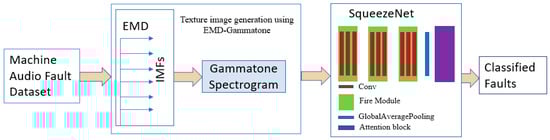
Figure 1.
Detailed block diagram of the proposed methodology.
The self-attention architecture, as depicted in [], consists of a self-attention layer preceded by two 2D convolutional layers with three fire modules in between, and a global max pooling layer. The self-attention layer is responsible for computing the logits. The fire module is one of the core components of our model. It comprises three convolutional layers. The first layer is a 1 × 1 convolution that reduces the number of filters to the “squeeze” parameter, followed by two parallel convolutional layers: one 1 × 1 convolution and one 3 × 3 convolution. These layers each produce “expand//2” filters. The outputs of these parallel layers are concatenated to form the final output of the fire module. This design reduces the computational complexity while maintaining rich feature extraction capabilities.
The total trainable parameters of the SqueezeNet architecture is 73,632 and with additional attention blocks, this increases to a maximum of 82,224. The model is lightweight compared to the state-of-the-art architectures, where the trainable parameters of CNN [,], DenseNet151 [], ResNet50 [], and VGG16 [] are 1.3 million, 20 million, 23 million, and 138 million, respectively.
| Algorithm 1: Steps followed to implement the proposed fault detection model |
Step 1: Signal pre-processing and texture image generation
|
The encoder model begins with an input layer that accepts tensors of the specified input shape. This input is then processed through an initial convolutional layer with a 3 × 3 kernel and 16 filters, utilizing ‘ReLU’ activation and the same padding. Following this, the data are passed through a sequence of three fire modules, which are innovative structures combining 1 × 1 and 3 × 3 convolutions to balance complexity and performance, with the first module configured with 24 squeezes and 48 expand filters, and the subsequent two modules each with 48 squeezes and 96 expand filters. After each of the first two fire modules, a MaxPooling2D layer with a pool size of 2 is applied to reduce the spatial dimensions. After the third fire module, another convolutional layer with a 3 × 3 kernel and 16 filters is applied. The output of this layer is then subjected to global average pooling, reducing the feature map to a single value per filter. This pooled output is processed by a multi-head attention layer with two heads and a key dimension of 64, focusing attention across one axis and outputting the transformed tensor along with attention scores. Finally, the resulting tensor is fed into a dense layer with a softmax activation function to produce the class probabilities.
The following subsections present the channel details, CBAM, and spatial attention mechanisms.
2.1. Channel Attention Mechanism
After passing through convolutional layers, the channel attention produces a multi-channel feature map, [], where C, H, and W represent the number of channels, height, and width of the feature map, respectively. The information of each channel is different. The channel attention uses the relationship between the feature map of each channel to learn a one-dimensional weight, , and then multiply it with the respective channel. With the above principle, the channel attention mechanism focuses on more meaningful information. In [], the channel attention is computed as follows:
where stands for the sigmoid function, , and . The MLP weights ( and are shared for inputs and the ‘relu’ activation function is followed by . The channel attention module is presented in Figure 2, where both the average pooled and max pooled features are used simultaneously.
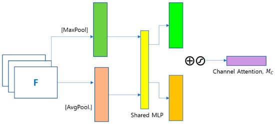
Figure 2.
Channel Attention module.
2.2. Spatial Attention Mechanism
The spatial attention mechanism [,] assigns a higher weight to the more informative features of each frame. Figure 3 shows the spatial attention mechanism, where Max-pooling and Global average pooling are applied to the feature map, and F is applied to interpret the features. Then, a convolution layer with a kernel size of 3 and a filter size of 16, along with the ‘relu’ activation function, is applied to calculate the attention map, . The is calculated as [],
where is sigmoid function and is used for a convolutional operation with a filter size of 3 × 3.
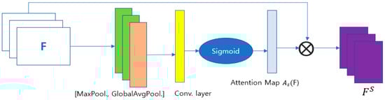
Figure 3.
Spatial attention mechanism.
2.3. CBAM Attention Mechanism
The CBAM has two sequential sub-modules, namely channel and spatial []. Considering an intermediate input feature map, , CBAM sequentially infers a one-dimensional channel attention map, , and a two-dimensional spatial attention map, . The attention processing can be expressed as
where stands for element-wise multiplication. is the final refined output and, during the multiplication, channel attention values broadcast along with the spatial dimension and vice versa. Figure 4 illustrates the detailed blocks associated with the CBAM mechanism.
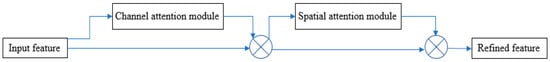
Figure 4.
CBAM Attention Mechanism with channel and spatial attention module.
3. Experimental Results Analysis
The following subsections present the results of different experiments performed with the lightweight SqueezeNet followed by four attention mechanisms. All the simulation results are collected by running the model for 200 epochs both for MIMII [] and ToyADMOS []. The MIMII dataset consists of eight classes, including normal and abnormal faults in a fan, pump, slider, and valve. In Figure 5 and Figure 6, 0 stands for fan abnormal, 1 for fan normal, 2 for pump abnormal, 3 for pump normal, 4 for slider abnormal, 5 for slider normal, 6 for valve abnormal, and 7 for valve normal. In all cases, normal samples are almost 3 times higher than the abnormal fault samples; details of the number of samples are presented in []. There are three types of machines in ToyADMOS, namely toy car, toy conveyor, and toy train, where each machine has normal and abnormal faults. Compared to the MIMII dataset, ToyADMOS is an imbalanced dataset, as the total samples for toy car is 6573, where 250 and 150 samples are for toy train and toy conveyer, respectively. During dataset preparation, a sample with a size of 1024 is taken from each large sample signal. To sift out the high-frequency constituents from the input signal, we selected the top six IMFs for generating a combined signal. Then, we applied the gammatone spectrogram to generate a spectrogram texture image. Then, after resizing the spectrogram image to 32 × 32, the input images were fed to the architectures for training and testing the model. As performance metrics, we utilized precision, recall, F1-score, and confusion matrix. In addition to the different metrics, different visualization curves such as the training and validation accuracy, loss curves, ROC curves, and t-SNE were used to explain the results of the model with four different attention mechanisms.
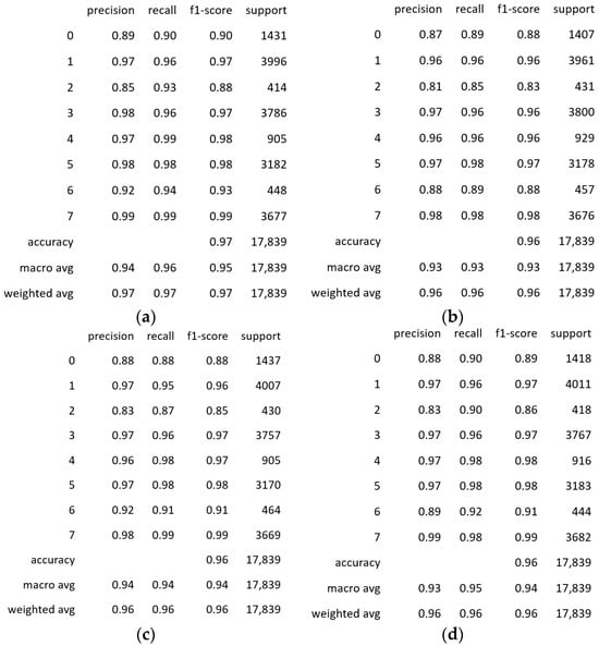
Figure 5.
Detailed accuracy results: precision, recall and F1-score of (a) self-attention, (b) CBAM, (c) channel, and (d) spatial attention mechanisms for the MIMII dataset.
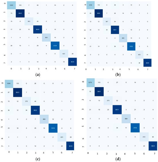
Figure 6.
Detailed confusion matrix of (a) self-attention, (b) CBAM, (c) channel, and (d) spatial attention mechanisms for the MIMII dataset.
3.1. Experiment with MIMII Dataset
The performance of various modified SqueezeNet models was evaluated on the MIMII dataset. Table 2 presents the results of these models, including the number of trainable parameters, accuracy, and f1-score for each model.
Table 2.
Classification report of the tested models for the MIMII dataset.
The SqueezeNet model integrated with self-attention exhibited a superior performance compared to the other models. It achieved the highest accuracy of 97% and an F1-score of 0.97, indicating that the self-attention mechanism enhances the model’s ability to identify faults accurately. The other models, which incorporated channel attention, spatial attention, and CBAM attention, all achieved an accuracy of 96% and an F1-score of 0.96, demonstrating their effectiveness but not matching the performance of the self-attention model.
Furthermore, as shown in Figure 7, the validation loss and accuracy curves for the self-attention SqueezeNet model were more stable compared to those of the other models. This stability suggests that the self-attention mechanism contributes to a more consistent training process, reducing fluctuations in model performance and leading to more reliable fault diagnosis results. Figure 8 shows the ROC curve of the self-attention SqueezeNet model, which were almost similar to the other attention mechanisms.
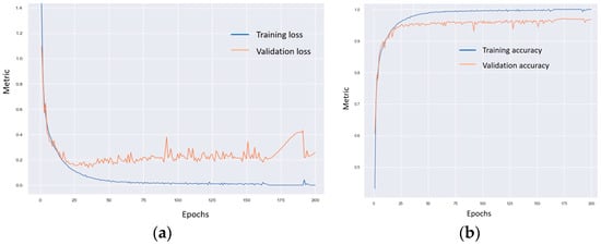
Figure 7.
Training and validation loss and accuracy curves for the self-attention mechanism: (a) loss curve and (b) accuracy curve for the MIMII dataset.
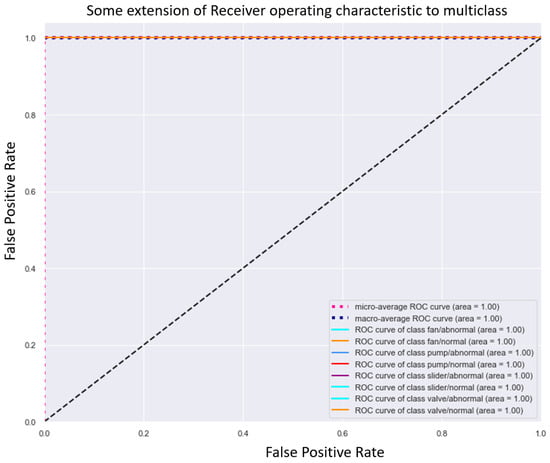
Figure 8.
ROC curve of self-attention mechanism for the MIMII dataset.
3.2. Experiment with ToyADMOS
The performance of different modified SqueezeNet models was assessed using the ToyADMOS dataset. Table 3 summarizes the results, highlighting the number of trainable parameters, accuracy, and F1-score for each model. In Figure 9 and Figure 10, 0 stands for car abnormal, 1 for car normal, 2 for conveyer abnormal, 3 for conveyer normal, 4 for train abnormal, and 5 for train normal.
Table 3.
Details of the classification report for the models tested using the ToyADMOS dataset.
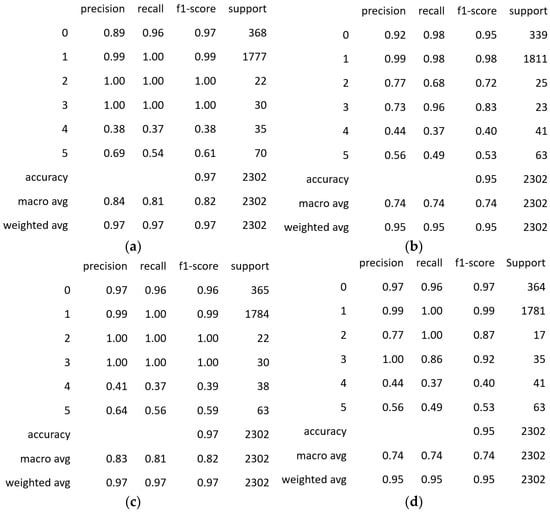
Figure 9.
Accuracy results: precision, recall and F1 score of (a) self-attention, (b) CBAM, (c) channel, and (d) spatial attention mechanisms for the ToyADMOS dataset.
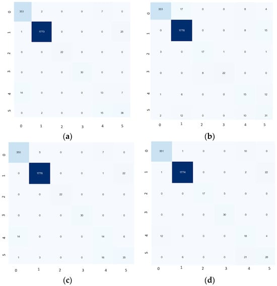
Figure 10.
Confusion matrix of (a) self-attention, (b) CBAM, (c) channel, and (d) spatial attention mechanisms for the ToyADMOS dataset.
As depicted in Figure 9, both the SqueezeNet model with self-attention and the one with channel attention achieved an accuracy of 97% and an F1-score of 0.97 on the ToyADMOS dataset, which were the highest values. This highlights that the self-attention and channel attention mechanisms both significantly enhance the model’s fault identification capabilities. The models with spatial attention and CBAM attention demonstrated a strong performance as well, with accuracies of 96% and 95%, and F1-scores of 0.96 and 0.95, respectively. These results confirm the effectiveness of these attention mechanisms, though they fell short of the self-attention and channel attention models’ performance.
Additionally, the validation loss and accuracy curves (as shown in Figure 11) for the self-attention SqueezeNet model were more stable compared to the other models. This indicates that the self-attention mechanism contributes to a more consistent training process, reducing performance fluctuations and resulting in more reliable fault diagnosis outcomes.
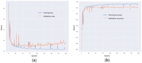
Figure 11.
Training and validation loss and accuracy curves of the self-attention mechanism: (a) loss curve and (b) accuracy curve for the ToyADMOS dataset.
However, it is important to note that the ToyADMOS dataset exhibited extreme class imbalance, posing a significant challenge for the models, particularly in handling minority classes. The models, including those with self-attention and channel attention, struggled considerably to accurately identify faults in these underrepresented classes, impacting their overall performance and highlighting an area for further improvement in future research. Like the MIMII dataset, the ROC curve of the self-attention SqueezeNet model for ToyADMOS was almost similar to the other attention mechanisms, as shown in Figure 12.
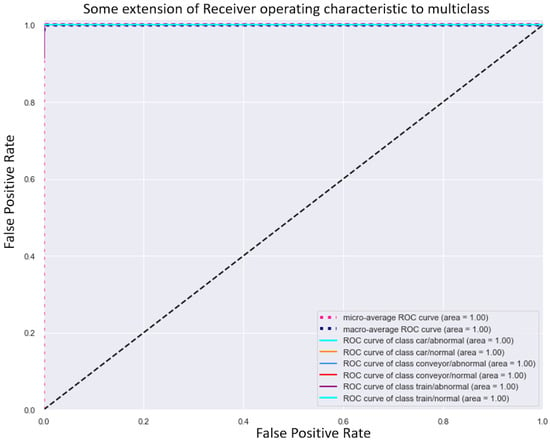
Figure 12.
ROC curve of self-attention mechanism for the ToyADMOS dataset.
4. Interpretation of Self-Attention SqueezeNet Results with T-SNE
Figure 13 and Figure 14 exhibit t-SNE plots of the self-attention SqueezeNet logits using the MIMII and ToyADMOS dataset, respectively. The plots were generated at 100-epoch intervals throughout the 200-epoch training session. The figures also include two additional plots: one representing the t-SNE plot with no training (epoch 0) and the other depicting the t-SNE plot on the test set of MIMII and ToyADMOS.
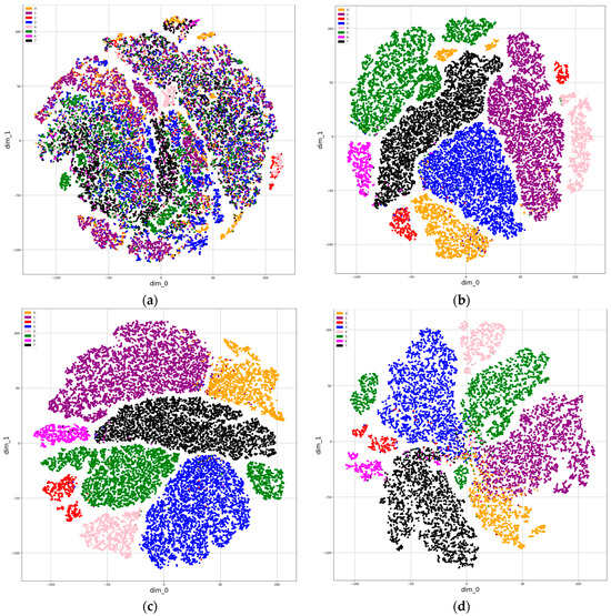
Figure 13.
tSNE plots of self-attention SqueezeNet logits using the MIMII dataset: (a) 0 epochs, (b) 100 epochs, (c) 200 epochs, (d) test set features after training.
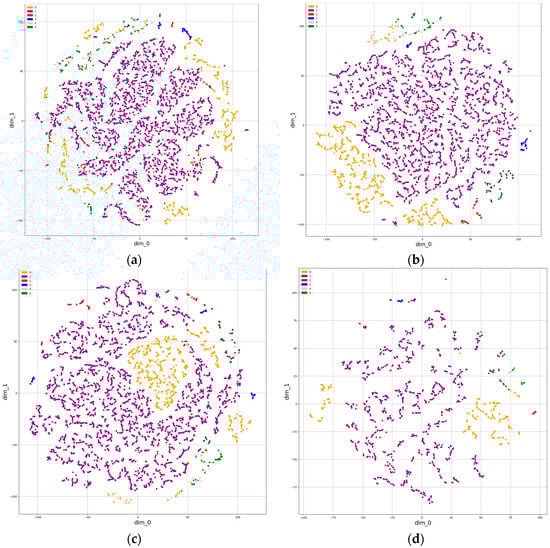
Figure 14.
tSNE plots of self-attention SqueezeNet logits using the ToyADMOS dataset: (a) 0 epochs, (b) 100 epochs, (c) 200 epochs, (d) test set features after training.
These visualizations provide insights into how the model’s feature space evolves during training and its effectiveness in differentiating between classes. The progression of the t-SNE plots over the epochs highlights the model’s ability to learn and separate different fault types more distinctly as training progresses. The comparison between the training and test set t-SNE plots further demonstrates the model’s generalization capability.
The t-SNE plots in Figure 13 demonstrate a clear separation of clusters representing different fault types. This indicates that the self-attention SqueezeNet model effectively learned to distinguish between various fault categories, with the separation becoming more distinct as training progressed. These well-defined clusters in the feature space highlight the model’s robust capacity for fault identification and classification.
In contrast to Figure 13, Figure 14 shows the t-SNE plots of the self-attention SqueezeNet logits using the ToyADMOS dataset. Here, the clusters representing different fault types are less clearly separated. This observation is primarily attributed to the class imbalance present in the ToyADMOS dataset, where certain fault types are underrepresented compared to others. This imbalance poses a challenge for the model in learning distinct representations for minority classes, resulting in fewer distinct clusters in the feature space visualization.
Despite these challenges, the t-SNE plots in Figure 14 still provide valuable insights into the model’s learning process and its attempt to differentiate between fault types. Addressing class imbalance through techniques like data augmentation or class weighting could potentially improve the model’s performance on datasets such as ToyADMOS, enabling the clearer separation of clusters and enhancing the overall fault classification accuracy.
5. Conclusions
While the model is designed to be computationally efficient, the incorporation of multi-head attention mechanisms still introduces a non-negligible computational overhead. This could be a constraint when deploying the model on resource-limited portable devices. The further optimization and exploration of lightweight attention mechanisms could mitigate this issue. Moreover, the ToyADMOS dataset’s class imbalance significantly impacted the model’s performance, particularly for minority classes. Although the model achieved high accuracy overall, its ability to accurately identify faults in underrepresented classes was diminished.
In conclusion, this paper presented a comparative analysis of four attention mechanisms: self-attention, channel, spatial, and CBAM. All the experiments were run using two public datasets: MIMII and ToyADMOS. Among the attention mechanisms, the self-attention mechanism accurately extracts more useful information from the fault datasets. The experimental results show that the additional self-attention blocks do not increase the number of trainable parameters in the overall architecture and that the self-attention mechanism demonstrates a 0.97 F1-score, whereas the other three mechanisms show a 0.96 F1 score for the MIMII dataset. For the ToyADMOS dataset, self-attention demonstrates a 0.97 F1-score, whereas the channel, spatial, and CBAM exhibit F1-scores of 0.97, 0.96, and 0.95, respectively. The results demonstrate that the self-attention SqueezeNet model achieved the highest accuracy and F1-scores on both datasets, indicating its superior fault identification capabilities.
The limitations of this study are that the model is tested with an imbalanced dataset and that the computational complexity of it is only determined with trainable parameters. In the future, data imbalance issues could be handled with data augmentation techniques and the model’s computational complexity could be addressed using optimal feature selection with explainable AI techniques.
Author Contributions
Conceptualization, M.Z.; methodology, M.Z.; software, M.Z.; validation and visualization, M.Z., A.N.B.K. and M.K.K.; formal analysis, M.Z. and M.K.K.; data curation, M.Z. and M.K.K.; writing—original draft preparation, M.Z. and M.K.K.; writing—review and editing, H.-J.C. and J.U.; supervision, H.-J.C.; funding acquisition, H.-J.C. All authors have read and agreed to the published version of the manuscript.
Funding
This research was supported and funded by the Korean National Police Agency. [Project Name: XR Counter-Terrorism Education and Training Test Bed Establishment/Project Number: PR08-04-000-21].
Data Availability Statement
To validate the model, we have used two publicly available audio machine fault datasets: MIMII (https://zenodo.org/record/3384388, accessed on 5 June 2024) and ToyADMOS (https://zenodo.org/record/3351307#.XT-JZ-j7QdU, accessed on 5 June 2024).
Conflicts of Interest
The authors declare no conflicts of interest.
References
- Liu, R.; Yang, B.; Zio, E.; Chen, X. Artificial intelligence for fault diagnosis of rotating machinery: A review. Mech. Syst. Signal Process. 2018, 108, 33–47. [Google Scholar] [CrossRef]
- Xu, L.; Teoh, S.S.; Ibrahim, H. A deep learning approach for electric motor fault diagnosis based on modified InceptionV3. Sci. Rep. 2024, 14, 12344. [Google Scholar] [CrossRef] [PubMed]
- Siraj, F.M.; Ayon, S.T.K.; Samad, M.A.; Uddin, J.; Choi, K. Few-Shot Lightweight SqueezeNet Architecture for Induction Motor Fault Diagnosis using Limited Thermal Image Dataset. IEEE Access 2024, 12, 50986–50997. [Google Scholar] [CrossRef]
- Kankar, P.K.; Sharma, S.C.; Harsha, S.P. Fault diagnosis of ball bearings using machine learning methods. Expert Syst. Appl. 2011, 38, 1876–1886. [Google Scholar] [CrossRef]
- Sobie, C.; Freitas, C.; Nicolai, M. Simulation-driven machine learning: Bearing fault classification. Mech. Syst. Signal Process. 2018, 99, 403–419. [Google Scholar] [CrossRef]
- Liu, Y.; Yan, X.; Zhang, C.A.; Liu, W. An ensemble convolutional neural networks for bearing fault diagnosis using multi-sensor data. Sensors 2019, 19, 5300. [Google Scholar] [CrossRef]
- Zhang, R.; Peng, Z.; Wu, L.; Yao, B.; Guan, Y. Fault diagnosis from raw sensor data using deep neural networks considering temporal coherence. Sensors 2017, 17, 549. [Google Scholar] [CrossRef] [PubMed]
- Guo, M.; Liu, H.; Xu, Y.; Huang, Y. Building extraction based on U-Net with an attention block and multiple losses. Remote Sens. 2020, 12, 1400. [Google Scholar] [CrossRef]
- Woo, S.; Park, J.; Lee, J.Y.; Kweon, I.S. Cbam: Convolutional block attention module. In Proceedings of the 2018 European Conference on Computer Vision (ECCV), Munich, Germany, 8–14 September 2018; pp. 3–19. [Google Scholar]
- He, A.; Li, T.; Li, N.; Wang, K.; Fu, H. CABNet: Category attention block for imbalanced diabetic retinopathy grading. IEEE Trans. Med. Imaging 2020, 40, 143–153. [Google Scholar] [CrossRef]
- Zhang, H.; Wu, C.; Zhang, Z.; Zhu, Y.; Lin, H.; Zhang, Z.; Sun, Y.; He, T.; Mueller, J.; Manmatha, R.; et al. Resnest: Split-attention networks. In Proceedings of the IEEE/CVF Conference on Computer Vision and Pattern Recognition, New Orleans, LA, USA, 18–24 June 2022; pp. 2736–2746. [Google Scholar]
- Chen, L.; Zhang, H.; Xiao, J.; Nie, L.; Shao, J.; Liu, W.; Chua, T.S. Sca-cnn: Spatial and channel-wise attention in convolutional networks for image captioning. In Proceedings of the IEEE Conference on Computer Vision and Pattern Recognition, Honolulu, HI, USA, 21–26 July 2017; pp. 5659–5667. [Google Scholar]
- Akbar, A.S.; Fatichah, C.; Suciati, N. Single level UNet3D with multipath residual attention block for brain tumor segmentation. J. King Saud. Univ.—Comput. Inf. Sci. 2022, 34, 3247–3258. [Google Scholar] [CrossRef]
- Huang, J.; Chen, B.; Yao, B.; He, W. ECG arrhythmia classification using STFT-based spectrogram and convolutional neural network. IEEE Access 2019, 7, 92871–92880. [Google Scholar] [CrossRef]
- Islam, M.M.; Kim, J.M. Automated bearing fault diagnosis scheme using 2D representation of wavelet packet transform and deep convolutional neural network. Comput. Ind. 2019, 106, 142–153. [Google Scholar] [CrossRef]
- Shao, S.; McAleer, S.; Yan, R.; Baldi, P. Highly accurate machine fault diagnosis using deep transfer learning. IEEE Trans. Ind. Inform. 2018, 15, 2446–2455. [Google Scholar] [CrossRef]
- Wen, L.; Li, X.; Li, X.; Gao, L. A new transfer learning based on VGG-19 network for fault diagnosis. In Proceedings of the 2019 IEEE 23rd International Conference on Computer Supported Cooperative Work in Design (CSCWD), Porto, Portugal, 6–8 May 2019; pp. 205–209. [Google Scholar]
- Zhang, D.; Zhou, T. Deep convolutional neural network using transfer learning for fault diagnosis. IEEE Access 2021, 9, 43889–43897. [Google Scholar] [CrossRef]
- Guo, L.; Lei, Y.; Xing, S.; Yan, T.; Li, N. Deep convolutional transfer learning network: A new method for intelligent fault diagnosis of machines with unlabeled data. IEEE Trans. Ind. Electron. 2018, 66, 7316–7325. [Google Scholar] [CrossRef]
- Yang, B.; Lei, Y.; Jia, F.; Xing, S. An intelligent fault diagnosis approach based on transfer learning from laboratory bearings to locomotive bearings. Mech. Syst. Signal Process. 2019, 122, 692–706. [Google Scholar] [CrossRef]
- Zhang, R.; Tao, H.; Wu, L.; Guan, Y. Transfer learning with neural networks for bearing fault diagnosis in changing working conditions. IEEE Access 2017, 5, 14347–14357. [Google Scholar] [CrossRef]
- Han, T.; Liu, C.; Wu, R.; Jiang, D. Deep transfer learning with limited data for machinery fault diagnosis. Appl. Soft Comput. 2021, 103, 107150. [Google Scholar] [CrossRef]
- Li, G.; Wu, J.; Deng, C.; Wei, M.; Xu, X. Self-supervised learning for intelligent fault diagnosis of rotating machinery with limited labeled data. Appl. Acoust. 2022, 191, 108663. [Google Scholar] [CrossRef]
- Berenji, A.; Taghiyarrenani, Z.; Rohani Bastami, A. Fault identification with limited labeled data. J. Vib. Control 2024, 30, 1502–1510. [Google Scholar]
- Wei, M.; Liu, Y.; Zhang, T.; Wang, Z.; Zhu, J. Fault diagnosis of rotating machinery based on improved self-supervised learning method and very few labeled samples. Sensors 2021, 22, 192. [Google Scholar] [CrossRef]
- Tang, H.; Gao, S.; Wang, L.; Li, X.; Li, B.; Pang, S. A novel intelligent fault diagnosis method for rolling bearings based on Wasserstein generative adversarial network and Convolutional Neural Network under Unbalanced Dataset. Sensors 2021, 21, 6754. [Google Scholar] [CrossRef] [PubMed]
- Islam, R.; Uddin, J.; Kim, J.M. Texture analysis based feature extraction using Gabor filter and SVD for reliable fault diagnosis of an induction motor. Int. J. Inf. Technol. Manag. 2018, 17, 20–32. [Google Scholar] [CrossRef]
- Zabin, M.; Choi, H.J.; Uddin, J.; Furhad, M.H.; Ullah, A.B. Industrial Fault Diagnosis using Hilbert Transform and Texture Features. In Proceedings of the 2021 IEEE International Conference on Big Data and Smart Computing (BigComp), Jeju Island, Korea, 17–20 January 2021; pp. 121–128. [Google Scholar]
- Fan, H.; Ren, Z.; Zhang, X.; Cao, X.; Ma, H.; Huang, J. A gray texture image data-driven intelligent fault diagnosis method of induction motor rotor-bearing system under variable load conditions. Measurement 2024, 233, 114742. [Google Scholar] [CrossRef]
- Tran, M.Q.; Liu, M.K.; Tran, Q.V.; Nguyen, T.K. Effective fault diagnosis based on wavelet and convolutional attention neural network for induction motors. IEEE Trans. Instrum. Meas. 2021, 71, 3139706. [Google Scholar] [CrossRef]
- Chen, L.; Ma, Y.; Wang, H.; Wen, S.; Guo, L. A novel deep convolutional neural network and its application to fault diagnosis of the squirrel-cage asynchronous motor under noisy environment. Meas. Sci. Technol. 2023, 34, 115113. [Google Scholar] [CrossRef]
- Liu, H.; Li, L.; Ma, J. Rolling Bearing Fault Diagnosis Based on STFT-Deep Learning and Sound Signals. Shock Vib. 2016, 1, 6127479. [Google Scholar] [CrossRef]
- Benkedjouh, T.; Zerhouni, N.; Rechak, S. Deep Learning for Fault Diagnosis based on short-time Fourier transform. In Proceedings of the 2018 International Conference on Smart Communications in Network Technologies (SaCoNeT), El Oued, Algeria, 27–31 October 2018; pp. 288–293. [Google Scholar]
- Du, Y.; Wang, A.; Wang, S.; He, B.; Meng, G. Fault diagnosis under variable working conditions based on STFT and transfer deep residual network. Shock Vib. 2020, 1, 1274380. [Google Scholar] [CrossRef]
- Ahmed, H.O.; Nandi, A.K. Connected components-based colour image representations of vibrations for a two-stage fault diagnosis of roller bearings using convolutional neural networks. Chin. J. Mech. Eng. 2021, 34, 37. [Google Scholar] [CrossRef]
- Pham, M.T.; Kim, J.M.; Kim, C.H. Rolling bearing fault diagnosis based on improved GAN and 2-D representation of acoustic emission signals. IEEE Access 2022, 10, 78056–78069. [Google Scholar]
- Qin, Z.; Huang, F.; Pan, J.; Niu, J.; Qin, H. Improved Generative Adversarial Network for Bearing Fault Diagnosis with a Small Number of Data and Unbalanced Data. Symmetry 2024, 16, 358. [Google Scholar] [CrossRef]
- Zabin, M.; Kabir, A.N.B.; Kabir, M.K.; Choi, H.J.; Uddin, J. Machine Fault Diagnosis Using EMD-Gammatone Texture Representation and A Lightweight Self-Attention SqueezeNet. In Proceedings of the 2024 IEEE International Conference on Big Data and Smart Computing (BigComp), Bangkok, Thailand, 18–21 February 2024; pp. 32–39. [Google Scholar]
- Jung, H.; Choi, S.; Lee, B. Rotor Fault Diagnosis Method Using CNN-Based Transfer Learning with 2D Sound Spectrogram Analysis. Electronics 2023, 12, 480. [Google Scholar] [CrossRef]
- Ruan, D.; Wang, J.; Yan, J.; Gühmann, C. CNN parameter design based on fault signal analysis and its application in bearing fault diagnosis. Adv. Eng. Inform. 2023, 55, 101877. [Google Scholar] [CrossRef]
- Lin, S.L. Intelligent fault diagnosis and forecast of time-varying bearing based on deep learning VMD-DenseNet. Sensors 2021, 21, 7467. [Google Scholar] [CrossRef]
- Wen, L.; Li, X.; Gao, L. A transfer convolutional neural network for fault diagnosis based on ResNet-50. Neural Comput. Appl. 2020, 32, 6111–6124. [Google Scholar] [CrossRef]
- Su, J.; Wang, H. Fine-Tuning and Efficient VGG16 Transfer Learning Fault Diagnosis Method for Rolling Bearing. In Proceedings of the IncoME-VI and TEPEN 2021, Performance Engineering and Maintenance Engineering; Springer: Berlin/Heidelberg, Germany, 2022; pp. 453–461. [Google Scholar]
- Li, H.; Qiu, K.; Chen, L.; Mei, X.; Hong, L.; Tao, C. SCAttNet: Semantic segmentation network with spatial and channel attention mechanism for high-resolution remote sensing images. IEEE Geosci. Remote Sens. Lett. 2020, 18, 905–909. [Google Scholar] [CrossRef]
- Park, J.; Woo, S.; Lee, J.Y.; Kweon, I.S. A simple and light-weight attention module for convolutional neural networks. Int. J. Comput. Vis. 2020, 128, 783–798. [Google Scholar] [CrossRef]
- Cao, G.; Luo, S. Multimodal perception for dexterous manipulation. In Tactile Sensing, Skill Learning, and Robotic Dexterous Manipulation; Academic Press: Cambridge, MA, USA, 2022; pp. 45–58. [Google Scholar]
- Tanabe, R.; Purohit, H.; Dohi, K.; Endo, T.; Nikaido, Y.; Nakamura, T.; Kawaguchi, Y. MIMII DUE: Sound dataset for malfunctioning industrial machine investigation and inspection with domain shifts due to changes in operational and environmental conditions. In Proceedings of the 2021 IEEE Workshop on Applications of Signal Processing to Audio and Acoustics (WASPAA), New Paltz, NY, USA, 17–20 October 2021; pp. 21–25. [Google Scholar]
- Koizumi, Y.; Saito, S.; Uematsu, H.; Harada, N.; Imoto, K. ToyADMOS: A dataset of miniature-machine operating sounds for anomalous sound detection. In Proceedings of the 2021 IEEE Workshop on Applications of Signal Processing to Audio and Acoustics (WASPAA), New Paltz, NY, USA, 17–20 October 2021; pp. 313–317. [Google Scholar]
Disclaimer/Publisher’s Note: The statements, opinions and data contained in all publications are solely those of the individual author(s) and contributor(s) and not of MDPI and/or the editor(s). MDPI and/or the editor(s) disclaim responsibility for any injury to people or property resulting from any ideas, methods, instructions or products referred to in the content. |
© 2024 by the authors. Licensee MDPI, Basel, Switzerland. This article is an open access article distributed under the terms and conditions of the Creative Commons Attribution (CC BY) license (https://creativecommons.org/licenses/by/4.0/).