An Efficient and Accurate Ground-Based Synthetic Aperture Radar (GB-SAR) Real-Time Imaging Scheme Based on Parallel Processing Mode and Architecture

Abstract

When performing high-resolution imaging with ground-based synthetic aperture radar (GB-SAR) systems, the data collected and processed are vast and complex, imposing higher demands on the real-time performance and processing efficiency of the imaging system. Yet a very limited number of studies have been conducted on the real-time processing method of GB-SAR monitoring data. This paper proposes a real-time imaging scheme based on parallel processing models, optimizing each step of the traditional $\omega$K imaging algorithm in parallel. Several parallel optimization schemes are proposed for the computationally intensive and complex interpolation part, including dynamic parallelism, the $Group$-$Nstream$ processing model, and the $Fthread$-$Group$-$Nstream$ processing model. The $Fthread$-$Group$-$Nstream$ processing model utilizes $Fthread$, $Group$, and $Nstream$ for the finer-grained processing of monitoring data, reducing the impact of the nested depth on the algorithm’s performance in dynamic parallelism and alleviating the issue of serial execution within the $Group$-$Nstream$ processing model. This scheme has been successfully applied in a synthetic aperture radar imaging system, achieving excellent imaging results and accuracy. The speedup ratio can reach 52.14, and the relative errors in amplitude and phase are close to 0, validating the effectiveness and practicality of the proposed schemes. This paper addresses the lack of research on the real-time processing of GB-SAR monitoring data, providing a reliable monitoring method for GB-SAR deformation monitoring.

1. Introduction

Ground-based synthetic aperture radar (GB-SAR) is a new type of radar system developed over the past two decades. It acquires a synthetic aperture by moving the radar at a constant speed along a linear track, thereby enhancing the system’s azimuth resolution and achieving high-resolution two-dimensional imaging. GB-SAR has found extensive applications in various fields, including ground deformation monitoring, foreign object detection (FOD) at airports, electromagnetic scattering measurement, and ground demonstration verification [1,2,3,4]. As the demand for large observation scenes and high resolution in GB-SAR systems continues to increase, challenges such as high data rates and complex implementation algorithms have become more pronounced. These issues significantly escalate the processing platform’s load and impose severe challenges for traditional signal-processing architectures. The real-time processing of high-frequency, continuous deformation monitoring data is crucial for early warnings for landslides and high-risk buildings, and it is also key for on-site emergency rescue. Therefore, the research on real-time processing technology is of significant importance. However, there has been little research on real-time processing methods for GB-SAR monitoring data [2,5].

A key step in GB-SAR imaging is Range Cell Migration Correction (RCMC) [6,7,8]. At this stage, the coupling of echo data in azimuth and range directions necessitates the use of effective methods to avoid Doppler spectral overlap [9]. Due to their adoption of second-order Taylor expansions, traditional methods like the Range Doppler Algorithm (RDA) and the Chirp Scaling Algorithm (CSA) struggle to adapt to imaging scenes with large bandwidths, wide beam angles, and high squints. To mitigate the phase errors introduced by the second-order Taylor series expansion, it is necessary to expand the square root term in the spectrum to the third, fourth, or higher orders. This implies that the algorithm’s complexity will also rapidly increase with higher orders [10], and the phase-stationary point cannot be quickly calculated via the Principles Of the Stationary Phase (POSP), making it impossible to obtain the analytical expression of the system function in the 2D frequency domain and the range-Doppler domain. The $\omega$K algorithm ($\omega$KA) is a truly broadband, wide-beam, and large-squint imaging algorithm; it only utilizes POSP and Stolt mapping in the process of solving the 2D frequency spectrum analysis expression. $\omega$KA reconstructs scene images in the wave number domain, theoretically enabling complete focusing over the entire surveillance area [11,12]. Simultaneously, the $\omega$K algorithm corrects range–azimuth coupling through Stolt interpolation, effectively avoiding the drawbacks of RDA and CSA. Therefore, the $\omega$KA is more suitable for wideband, high-resolution GB-SAR imaging systems [13,14]. Stolt interpolation is commonly used in fields such as ultrasound and synthetic aperture imaging for nonlinear phase error correction [15,16,17,18,19]. Stolt interpolation achieves residual-range migration correction, residual secondary range compression, and residual azimuth compression through the mapping and warping of the range frequency axis [20]. Therefore, the computation of Stolt interpolation has a significant impact on the imaging accuracy and efficiency of the $\omega$KA, and it is necessary to perform precise calculations of Stolt interpolation within the imaging algorithm.

Stolt interpolation can be implemented using traditional methods such as splines, Piecewise Cubic Hermite Interpolating Polynomial (PCHIP), linear interpolation, or cubic interpolation [21]. However, these methods typically involve complex functions, resulting in a significant increase in the total computation time for image reconstruction. Therefore, many researchers often seek various improvements to avoid the complex computation of Stolt interpolation. For instance, Skouroliakou et al. [22] employs standard 3D techniques to replace Stolt interpolation and 3D IFT, as the 3D scene is a collection of 2D slices, which necessitates the computation of numerous 2D IFTs, adding a certain level of complexity to the algorithm’s implementation. Wang et al. [23] utilizes the sub-linear sampling complexity of 2D-BLSFT to reduce the interpolation times in the Stolt mapping step, thereby decreasing the complexity of Stolt interpolation from $O\left(L\times N_c\times N_r\right)$ to $O\left(L\times K\times log\left(N_c\right)\times log\left(N_r\right)\right)$. This method requires the imaged scene to exhibit sparsity, and 2D-BLSFT still incurs a certain computational cost. Both keystone interpolation and Stolt interpolation deal with three-dimensional data. Keystone interpolation can interpolate along a particular dimension [24], whereas Stolt interpolation involves two-dimensional known data and one-dimensional estimated data, and thus cannot interpolate along the estimated or known data. Additionally, Stolt interpolation can be replaced by phase multiplication for completing residual azimuth compression [25]. Although this approach avoids the complexity of interpolation, it requires the assumption that both residual range migration and residual range–azimuth coupling are range-invariant, and it is only effective at low squint angles and narrow swath widths. Therefore, a low-complexity Stolt interpolation scheme needs to be introduced [26].

The various modules within imaging algorithms exhibit a degree of independence and parallelism, enabling the acceleration of algorithms through high-performance techniques [27,28]. GPUs possess powerful parallel computing capabilities and high memory bandwidth, making them commonly used in accelerating synthetic aperture image processing [29,30,31]. They can enhance signal processing and imaging efficiency through task partitioning and scheduling, optimizing access conflicts, and fine-grained parallel pipelines [32,33]. For instance, Jin et al. [34] reconstructed multi-layered medium ultrasound full-matrix imaging using Stolt interpolation and accelerated it with a GeForce MX150 GPU, which, compared to FPGA-based hardware acceleration, demands simpler hardware requirements and is easier to implement. Yu et al. [35] proposed a wave-number domain synthetic aperture ultrasound image reconstruction method based on Stolt migration and accelerated it using a GeForce GTX 970 GPU, demonstrating its high computational efficiency. Wang et al. [23] designed the $\omega$K-BLSFT algorithm for SAR imaging, which reduces the complexity of stolt interpolation and shows the potential of parallel computing through GPU.

Therefore, this study proposes a real-time processing scheme for GB-SAR monitoring data, enabling continuous monitoring and the timely analysis of rapid surface deformations, as illustrated in Figure 1. The main contributions of this research are as follows: (a) three nested interpolation schemes are proposed through dynamic parallelism with multilayer kernel concurrency, which effectively achieves rapid processing of three-dimensional radar signals; (b) to reduce the impact of nested depth on the algorithm, the $Group$-$Nstream$ processing model is proposed based on the two-layer nested interpolation, dividing computational tasks into sub-tasks and processing them via $Group$s and $Nstream$s; (c) to address the issue of serial execution within $Group$s in the $Group$-$Nstream$ processing model, the $Fthread$-$Group$-$Nstream$ processing model is formed through hybrid programming with CUDA and OpenMP, providing a finer-grained interpolation processing of computational tasks via $Fthread$, $Group$, and $Nstream$; (d) the applicability and effectiveness of the proposed methods are validated through experimental tests with a W-band GB-SAR system, achieving good imaging results, significantly improving processing efficiency.

2. Signal Model

Assuming that the transmitted pulse of the synthetic aperture in the range direction is a linear frequency modulated (LFM) signal and the range equation is in the hyperbolic form as shown in Equation (1), then the baseband signal of a single point target after demodulation can be represented in the complex form shown in Equation (2).

$$R\left(\eta \right)=\sqrt{R_0^2-{\left(v\eta \right)}^2}$$

(1)

$$\begin{array}{c}{S}_0\left(\tau ,\eta \right)=A_0{w}_r\left(\tau -{\displaystyle \frac{2R\left(\eta \right)}{c}}\right)w_a\left(\eta -{\eta }_c\right)\times \hfill \\ exp\left\{-j4\pi f_0{\displaystyle \frac{R\left(\eta \right)}{c}}\right\}exp\left\{j\pi K{\left(\tau -{\displaystyle \frac{2R\left(\eta \right)}{c}}\right)}^2\right\}\hfill \end{array}$$

(2)

where c is the speed of light, v is the platform speed, K is the range modulation frequency, $R_0$ is the shortest distance from the target to the platform, $A_0$ is a constant term, and $w_r\left(\cdot \right)$ and $w_a\left(\cdot \right)$ are the range and azimuth pulse envelopes, respectively. By applying the principle of the stationary phase to perform the range Fourier transform and the azimuth Fourier transform on the received signal $S_0\left(\tau ,\eta \right)$, the two-dimensional frequency domain signal $S_{2d}\left(\tau ,\eta \right)$ can be obtained:

$$S_{2d}\left(f_{\tau },f_{\eta }\right)=A{W}_r\left(f_{\tau }\right)W_a\left(f_{\eta }-f_{\eta c}\right)EXP\left\{j{\theta }_{2d}\right\}$$

(3)

$${\theta }_{2d}\left(f_{\tau },f_{\eta }\right)=-{\displaystyle \frac{4\pi R_0}{c}}\sqrt{{(f_c+f_{\tau })}^2-{\displaystyle \frac{{\left(c{f}_{\eta }\right)}^2}{4v^2}}}-{\displaystyle \frac{\pi f_{\tau }^2}{K}}$$

(4)

where $f_{\tau }$ and $f_{\eta }$ are the range and azimuth frequencies, $f_{\eta c}$ is the Doppler center frequency, A is the constant term, and $W_r\left(f_{\tau }\right)$ and $W_a\left(f_{\eta }-f_{\eta c}\right)$ are the envelopes of the range spectrum and the azimuth spectrum, respectively. Since $R_0$ and v are defined in the time domain, when performing Reference Function Multiplication (RFM) in the two-dimensional frequency domain, it is necessary to use reference range and equivalent velocity. Therefore, the phase of the RFM filter is given by

$${\theta }_{ref}=+{\displaystyle \frac{4\pi R_{ref}}{c}}\sqrt{{(f_c+f_{\tau })}^2-{\displaystyle \frac{{\left(c{f}_{\eta }\right)}^2}{4v^2}}}+{\displaystyle \frac{\pi f_{\tau }^2}{K}}$$

(5)

The filter using the reference range $R_{ref}$ can only compensate for the phase and achieve complete focusing at the reference range $R_{ref}$, while residual phase errors ${\theta }_{RFM}$ exist at other range gates, resulting in non-linearities in the range frequency $f_{\tau }$. Under these circumstances, performing a range of IFFT will result in defocused imaging results [36]. The solution is to use Stolt mapping to map the range frequency $f_{\tau }$ to a new range frequency $f_{\tau }^{\prime }$ [25,36,37], as shown in Equation (7). It can be seen that the new frequency $f_{\tau }^{\prime }$ is linearly related to the residual phase, addressing non-linearities. ${\theta }_{stolt}$ represents the phase function after mapping, and the phase after Stolt mapping is linearly related to the new range frequency.

$${\theta }_{RFM}=-4\pi (R_0-R_{ref})/\phantom{(R_0-R_{ref})c\sqrt{{(f_0+f_{\tau })}^2-{\displaystyle \frac{c^2{f}_{\eta }^2}{4V_r^2}}}}c\sqrt{{(f_0+f_{\tau })}^2-{\displaystyle \frac{c^2{f}_{\eta }^2}{4V_r^2}}}$$

(6)

$$\sqrt{{(f_0+f_{\tau })}^2-{\displaystyle \frac{c^2{f}_{\eta }^2}{4V_r^2}}}=f_{\tau }^{\prime }+f_0$$

(7)

$${\theta }_{stolt}=-4\pi (R_0-R_{ref})(f_{\tau }^{\prime }+f_0)/\phantom{(R_0-R_{ref})(f_{\tau }^{\prime }+f_0)c}c$$

(8)

Stolt mapping alters the phase of data in the two-dimensional frequency domain while adjusting both azimuth and range phases, thus eliminating residual phase modulations of the second order and higher. Stolt interpolation is required to correct residual range cell migration, residual secondary range compression, and residual azimuth compression, which significantly impact the quality of imaging. Therefore, precise computation is necessary for the Stolt interpolation portion [38,39,40].

3. Data Preprocessing before Interpolation

Datasets and System Parameters

The experimental data were collected using a ground-based synthetic aperture radar system. This system is a W-band track SAR mounted on a linear track with a height of 2.5 m and a length of 9 m. The operating frequency is in the W band, ranging from 92 to 98 GHz, with an instantaneous bandwidth of 6 GHz. Other operating parameters are shown in

Table 1. Set of system parameters.

Parameter	Value
Carrier frequency ($fc$)	95 GHz
Bandwidth (B)	6 GHz
Pulse repetition frequency ($PRF$)	400 MHz
Real aperture (L)	6.05 m
Sampling frequency ($fs$)	2.5 MHz
Echo signal ($Na\times Nr$)	4610 × 8000
Radar speed	0.3025 m/s
Imaging range (R)	1 m–4 m
CPU	Intel i7-9750H
GPU	NVIDIA GeForce GTX 1660 Ti

. According to Table 1, the range resolution is ${\displaystyle \frac{0.886c}{2B}}=2.22$ cm, and the azimuth resolution is ${\displaystyle \frac{R\lambda }{2L}}\le 1$ cm. In this experiment, the system was used to achieve the high-resolution imaging of a sand table. The experiment was compared to the traditional $\omega$K imaging scheme, with the experimental data and environment kept consistent.

Figure 1 shows a schematic diagram of the real-time processing scheme. The echo data collected by the imaging system are stored in the CPU’s memory, located in the range frequency domain and azimuth time domain. First, the echo data need to be read and saved to the GPU’s memory. At this point, the imaging range is relatively short, and there is oversampling in both the azimuth and range directions, so extraction is required to reduce the sampling rate. The $\omega$K algorithm requires signal processing in the range or azimuth frequency domain as well as the two-dimensional frequency domain. Therefore, the imaging algorithm involves multiple row FFT/IFFT, column FFT/IFFT, and 2D FFT operations. In this scheme, row FFT/IFFT and column FFT/IFFT are designed using the CUFFT library and encapsulated into corresponding macro functions.

Before interpolation, the data are non-uniform and need to be resampled into uniform data using Stolt interpolation [17,26,41]. As shown in Figure 2, Shadow 1 indicates that the front end of the data after Stolt interpolation will protrude forward, exceeding the length of the echo signal. Therefore, zero-padding is required to increase the data length [34]. Shadow 2 represents the discard zone, where data in this area need to be discarded after interpolation.

As shown in

Table 2. Optimization of data preprocessing before interpolation.

Preprocessing		Data Size	GPU	CPU	Speedup
Data reading	col FFT	4608 × 8000	120.05 ms	1250.02 ms	10.41
	col IFFT	2304 × 8000	39.36 ms	754.12 ms	19.14
Azimuth extraction	col FFT	8000 × 2304	42.95 ms	1115.06 ms	25.96
	col IFFT	8000 × 2304	46.72 ms	1133.70 ms	24.27
	extraction	4000 × 2304	1.18 ms	120.14 ms	101.81
Range extraction	col FFT	4000 × 2304	12.32 ms	228.68 ms	18.56
	col IFFT	4000 × 2304	9.09 ms	266.86 ms	29.36
	extraction	4000 × 1152	2.98 ms	62.10 ms	20.84
Windowing and zero-padding	windowing and zero-padding in the range	4000 × 1152	1.03 ms	106.10 ms	103.01
	windowing in the azimuth	4000 × 1728	1.2309 ms	397.262 ms	322.98

, the runtime for windowing and zero-padding on the GPU and CPU is presented. On the GPU, range domain zero-padding and windowing are performed simultaneously. The speedup for range domain zero-padding and windowing on the GPU is 103.01, and for azimuth domain windowing, the speedup is 322.98. When running zero-padding and windowing kernel functions on the default stream, window functions and compensation functions need to be invoked. As illustrated in Figure 3, this paper adopts a dual-stream approach, where window functions and compensation functions are generated in advance through a non-blocking stream before the execution of kernel functions on the default stream. This allows the default stream to directly invoke the window functions when running zero-padding and windowing kernel functions, eliminating the need to wait for the generation of window functions as is necessary on the CPU, thereby significantly reducing the runtime of the imaging algorithm. As depicted in Figure 3, the primary function of the $get\_t$ kernel function is to generate the relevant parameters and functions required by the kernel functions on the default stream. It is evident that the generation of these parameters and functions can be entirely hidden within the data transfer process. The FFT/IFFT kernel functions for rows and columns on the CPU side in Table 2 are designed and encapsulated using the FFTW library. It is apparent that the FFT operations for rows and columns on the GPU exhibit better real-time performance. Performing FFT operations on the GPU helps avoid data transfer between the CPU and GPU, thereby significantly enhancing the speed and efficiency of the imaging algorithm.

4. Fine Parallel Implementation of Stolt Interpolation

4.1. Three Layers Dynamic Nesting Implementation Scheme

The object of Stolt interpolation is a set of three-dimensional signals with a size of $Na\times Nr\times Nr$, including two-dimensional known data of size $Na\times Nr$ and one-dimensional estimated data of size $1\times Nr$. Algorithmically, it manifests as a triple loop, implying that Stolt interpolation requires the implementation of multiple complex kernel functions with strict dependencies among them. If all these kernel functions’ workloads are controlled solely by the host, frequent interactions between the host and the device would be necessary. Therefore, the imaging algorithm needs to be designed as a separate, massively data-parallel kernel launch. Dynamic parallelism offers a more hierarchical approach, where concurrency can be exhibited across multiple levels within a GPU kernel. It dynamically leverages the GPU hardware scheduler and load balancer, adjusting to accommodate data-driven or workload changes [42]. The ability to create work directly on the GPU side reduces the need for transferring data and executing controls between the host and the device. Therefore, dynamic parallelism can be employed to realize Stolt interpolation. The triple loop implies that a dynamic parallel nesting with a depth of 3 can be achieved.

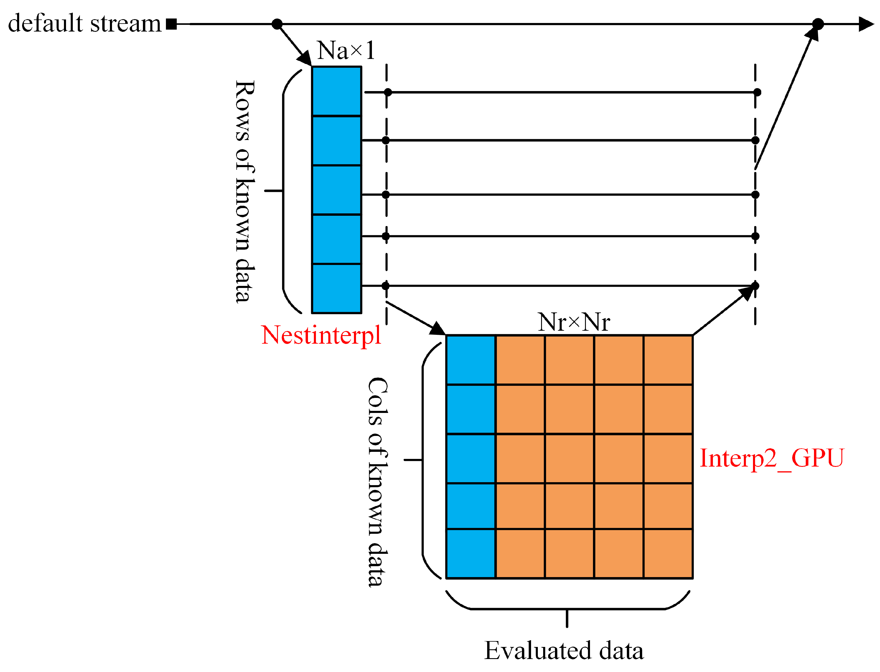
4.1.1. One-Layer Nested Interpolation

We have parallelized the sub-aperture imaging algorithm by performing interpolation in one direction from either the known data or the estimated data. In the parallelization of the sub-aperture imaging algorithm, the known data, which are one-dimensional, are in the real time domain, while the estimated data, in the virtual time domain, are two-dimensional. If interpolation is performed in the direction of the virtual time domain, the entire two-dimensional matrix can be traversed, compared, and interpolated simultaneously. Therefore, as long as the number of virtual time domain points does not exceed the GPU’s thread limit, the runtime theoretically remains constant. In the Stolt interpolation of the $\omega$K algorithm, the known data are two-dimensional, while the estimated data are one-dimensional, and the range of comparison for interpolation is each row within the known data. If all of the known data are traversed, compared, and interpolated simultaneously, there may be neighboring points closer to the estimated data outside specific rows, resulting in incorrect interpolation for those points and consequently incorrect interpolation for all of the estimated data. Therefore, in the $\omega$K algorithm, the Stolt interpolation part cannot simultaneously interpolate two-dimensional data but can be interpolated row by row, referred to as one-layer nested interpolation in this paper.

As shown in Figure 4, one-layer nested interpolation is applied to perform interpolation on a single point of two-dimensional known data in the frequency domain. Any known data point is compared with $Nr$ estimated data points simultaneously, and the nearest points are selected for linear fitting. The two-dimensional known data in Figure 4 are arranged row by row, with a total of $Na$ rows, each containing $Nr$ points, resulting in a total of $Na\times Nr$ points. Therefore, a total of $Na\times Nr$ interpolation operations are required.

4.1.2. Two-Layer Nested Interpolation

Figure 5 illustrates the working principle of two-layer nested interpolation. The kernel function $Nestinterp1$ serves as the parent kernel function, conducting parallel optimization on the rows of known data and completing the interpolation operation for each row. $Nestinterp1$ represents the first layer of nesting in two-layer nested interpolation. The kernel function $Interp2\_GPU$ is the child kernel function, responsible for the parallel optimization of the estimated data. During the execution of the parent kernel function $Nestinterp1$, each thread of the parent kernel function invokes $Interp2\_GPU$ to perform interpolation operations for $Nr$ rows of known data. The kernel function $interp2\_GPU$ completes the tasks of the second and third loops in the triple loop of the traditional Stolt interpolation method, making it the second layer of two-layer nested interpolation. $Interp2\_GPU$ does not optimize the columns of the known data but still executes serially, but three-layer nested interpolation will optimize this aspect.

4.1.3. Three-Layer Nested Interpolation

Three-layer nested interpolation optimizes both the rows and the columns of the known data in parallel. As shown in Figure 6, the kernel function $Interp\_lay2$, representing the second layer of three-layer nested interpolation, completes the traversal and indexing of the known data columns. $Interp\_lay1$, representing the third layer of three-layer nested interpolation, completes the traversal, comparison, and interpolation of the estimated data. $Interp\_lay2$ and $Interp\_lay1$ achieve the functionality of the child kernel function $Interp2\_GPU$ through nesting.

As shown in Section 5, both one-layer nested interpolation and two-layer nested interpolation result in performance acceleration, while three-layer nested interpolation takes longer than the CPU counterpart. Each device has a maximum nesting depth limit. In practice, real-time imaging algorithms require continuous, around-the-clock monitoring of deformable geological bodies, resulting in a massive amount of data. Initiating another grid within a new primary grid consumes additional memory resources, and the synchronization management across different layers demands a significant amount of device memory. In three-layer nested interpolation, a new grid $Interp\_lay2$ is created within all threads of the parent grid $Nestinterp1$, and all threads of $Interp\_lay2$ then initiate another new grid $Interp\_lay1$. This necessitates allocating additional memory resources to start the new grid and maintain synchronization between the old and new grids. Moreover, the deeper the nesting depth, the more frequent the synchronization requirements between layers. From Figure 5 and Figure 6, two-layer nested interpolation requires maintaining dependency and synchronization relationships between $Nestinterp1$ and $interp2\_GPU$. In contrast, three-layer nested interpolation requires maintaining dependency and synchronization relationships, including $Nestinterp1$-$Interp\_lay2$, $Nestinterp1$-$Interp\_lay2$, $Interp\_lay2$-$Interp\_lay1$, and $Nestinterp1$-$Interp\_lay2$-$Interp\_lay1$, which theoretically are four times that of two-layer nesting.

4.2. The Processing Mode of $Fthrea$-$Group$-$Nstream$

From Section 4.1, it can be inferred that one-layer nested interpolation lacks sufficient depth, while the dependencies and synchronization relations in three-layer nested interpolation are overly complex. Therefore, overall, two-layer nested interpolation is more suitable. The essence of two-layer nested interpolation is the parallel optimization of the first and third loops of the traditional Stolt interpolation method. To further reduce the dependencies and synchronization between layers, further optimization of the two-layer nested interpolation is required. For the first loop, we can replace the multi-threaded processing mode with a multi-stream approach. As shown in Figure 7, when optimizing the rows of known data, the parent kernel function $Nestinterp1$ needs to activate $Na$ threads. Since the number of streams that can be initiated is far lower than the number of threads, it is impractical to replace these $Na$ threads with $Na$ non-blocking streams ($Nstream$). Therefore, a set of streams needs to be executed multiple times to complete the tasks performed by these $Na$ threads. The $Group$ number and $Nstream$ number can accurately identify the points that need to be traversed and interpolated.

Each $Group$ contains several $Nstream$s, so it is necessary to partition the computational tasks and assign corresponding subtasks to each $Nstream$ within the $Group$s, as illustrated in Figure 8 and Equation (9). i and j represent the indices of the $Group$ and $Nstream$, respectively, that is, the $Nstream$ number and the $Group$ number. $add\_start\left(i,j\right)$ denotes the starting address of the subtask that the j-th $Nstream$ in the i-th $Group$ needs to process. The first layer of nesting in the two-layer nested interpolation is divided into $Ng$ $Group$s, with each $Group$ containing $Ns$ $Nstream$s. Each $Nstream$ within the same $Group$ contains $Nr$ threads that form a grid that implements the kernel function $interp2\_GPU$.

$$\left\{\begin{array}{c}Ng={\displaystyle \frac{Na}{Ns}}\\ add\_start\left(i,j\right)=(i\times Ng+j)\times Nr\\ \begin{array}{c}i=0,1,2,\cdots ,Ng-1\\ j=0,1,2,\cdots ,Ns-1\end{array}\end{array}\right.$$

(9)

$Group$s are executed sequentially, but they are independent of each other and hence exhibit a certain level of parallelism. Open Multi-Processing (OpenMP) is an application programming interface (API) and a mature and widely used compiler directive that provides support for parallel programming in shared-memory environments [43]. It offers advantages such as good portability, powerful functionality, and high computational efficiency, enabling parallel computing by partitioning computational regions [44,45,46]. Therefore, the parallel execution of $Group$s can be achieved through OpenMP. Figure 9 illustrates the Fork–Join parallel execution model of OpenMP, where the main thread spawns multiple threads for parallel computation; this process is known as Fork. When the parallel code execution is complete, the spawned threads either exit or are suspended, and the control flow returns to the standalone main thread, termed Join.

Introducing OpenMP to address the issue of serial execution of $Group$s leads to changes in both the partitioning and indexing of subtasks. Figure 1 and Figure 10 show a schematic diagram of task partitioning when the number of $Fthread$s is 2 and $Ng$ $Group$s are evenly distributed among $Hs$ fork threads ($Fthread$), with each fork thread handling the computation task of one $Group$. Completing all $Group$ computation tasks requires $Np$ parallel computations. As shown in Equation (10), the starting address of the data is now indexed by $Fthread$, $Group$, and $Nstream$. Here, k is the index of the fork thread.

$$\left\{\begin{array}{c}\begin{array}{c}Np={\displaystyle \frac{Ng}{Hs}}={\displaystyle \frac{Na}{Ns\times Hs}}\\ add\_start\left(i,j\right)=(i\times Ng+j)\times Nr\end{array}\\ k=0,1,2,\cdots ,Hs-1\\ \begin{array}{c}k\times Np\le i<\left(k+1\right)\times Np\\ j=0,1,2,\cdots ,Ns-1\end{array}\end{array}\right.$$

(10)

5. Field Experiment

5.1. Experimental Analysis

The maximum number of concurrent GPU kernels depends on the device and is limited by computational resources such as shared memory and registers [47]. If the number of streams exceeds the number of hardware connections, some streams will share a work queue, resulting in false dependencies. Hyper-Q technology maintains multiple hardware connections between the host and the device, allowing multiple GPU threads or processes to launch work on a single GPU simultaneously, thereby reducing false dependencies [42,48]. Starting from the Kepler architecture, the hardware work queue has been increased to 32, with different streams allocated to different queues, avoiding false dependencies. If more than 32 streams are created, the extra streams will share a hardware work queue with the other streams. Figure 11 illustrates the impact of the number of non-blocking streams on interpolation time under the parameters listed in Table 1; it can be observed that as the number of streams increases, the interpolation time decreases. When the number of streams reaches 25, the interpolation time stabilizes, and the acceleration effect saturates. Although this does not reach the limit of the hardware queue, the required resources exceed the device’s capabilities.

CUDA supports using multiple host threads to schedule operations to multiple streams, with one thread managing each stream. Therefore, we can use OpenMP to perform parallel optimization on the $Group$s. Compared to GPU threads, the number of host threads available for parallel execution is relatively limited. Additionally, the parallel execution of host threads is typically constrained by the physical cores and hyper-threading technology. Once this limit is exceeded, it is not possible to directly share threads or queues. Therefore, when the number of host threads executing in parallel exceeds the maximum supported by the CPU, the algorithm’s precision decreases. Unlike host threads, when the number of non-blocking streams exceeds the hardware queue, the excess streams share the hardware queue without affecting the precision of interpolation. Therefore, to improve the performance and precision of the algorithm, we can create more non-blocking streams, thereby reducing the number of threads that need to be activated by OpenMP.

According to Equation (10), $N\mathrm{s}$ must be a factor of $Na=4000$. From Figure 11, it can be seen that the acceleration effect stabilizes when $N\mathrm{s}=25$. Beyond 25, the acceleration effect becomes increasingly insignificant, reaching a peak when $N\mathrm{s}=50$. Therefore, let $N\mathrm{s}=50$, and $N\mathrm{g}=80$. $Hs$ must be a factor of 80, where $Hs$ represents the number of derived host threads. As shown in Figure 12, $interp2\_GPU$ represents a subtask. The non-blocking streams can execute these subtasks almost in parallel, with each stream executing multiple subtasks. Therefore, the execution times of $interp2\_GPU$ across different streams can overlap, thereby improving the algorithm’s runtime efficiency. As shown in

Table 3. The influence of the host thread count on algorithm performance and accuracy when the number of $Nstream$s is 50.

Platform	Number of Host Threads	Interpolation Time	Algorithm Runtime	Phase Relative Error	Amplitude Relative Error
Traditional $\omega$KA	1	29,070.4 ms	42,021.1 ms	0	0
Real-time imaging scheme	1	571.863 ms	1149.14 ms	$0\sim 1.93\times {10}^{-6}$	$0\sim 2.89\times {10}^{-9}$
	2	557.582 ms	1128.71 ms	$0\sim 1.93\times {10}^{-6}$	$0\sim 2.89\times {10}^{-9}$
	4	562.984 ms	1137.75 ms	$0\sim 1.93\times {10}^{-6}$	$0\sim 2.89\times {10}^{-9}$
	5	572.475 ms	1136.67 ms	$0\sim 1.93\times {10}^{-6}$	$0\sim 2.89\times {10}^{-9}$
	8	589.447 ms	1180.59 ms	$0\sim 1.93\times {10}^{-6}$	$0\sim 2.89\times {10}^{-9}$
	10	592.201 ms	1187.64 ms	$0\sim 1.93\times {10}^{-6}$	$0\sim 2.89\times {10}^{-9}$
	16	605.53 ms	1194.94 ms	$2.49\times {10}^{-10}\sim 906.37$	$1.5\times {10}^{-6}\sim 4.82$
	50	440.388 ms	1006.49 ms	$2.72\times {10}^{-7}\sim 1.86\times {10}^5$	$3.57\times {10}^{-5}\sim 1016.6$

, as $Hs$ increases, the consumption of CPU resources also increases. Additionally, the initiation and termination of host threads both impose a certain burden on the algorithm’s execution. The CPU used in this experiment is the Intel Core i7-9750H, which has six physical cores, with each core supporting two hyper threads. Therefore, the maximum number of parallel threads for this CPU is 12. When $Hs=16$, the imaging algorithm divides tasks and assigns and processes subtasks using 16 host threads. However, only a maximum of 12 host threads can be invoked, so only the subtasks executed by these 12 host threads can be correctly computed. The remaining four subtasks do not have corresponding threads available for invocation, resulting in errors in the final interpolation result. As shown in Figure 13, when $Hs=5$, the imaging error is primarily located in the region where the azimuth axis is 1−2 m. At this point, the maximum amplitude’s relative error is $2.89\times {10}^{-9}$, and the maximum phase’s relative error is $1.93\times {10}^{-6}$. When $Hs>12$, errors are present throughout the entire imaging scene, and the error increases as $Hs$ increases. When $Hs=40$, the maximum amplitude’s relative error is 165.4, and the maximum phase’s relative error is $1.38\times {10}^5$. The CPU cannot guarantee the invocation of all host threads for a particular computation, so the speed and accuracy of this algorithm also depend on the CPU’s performance. Choosing a CPU with better performance will further enhance the algorithm’s performance.

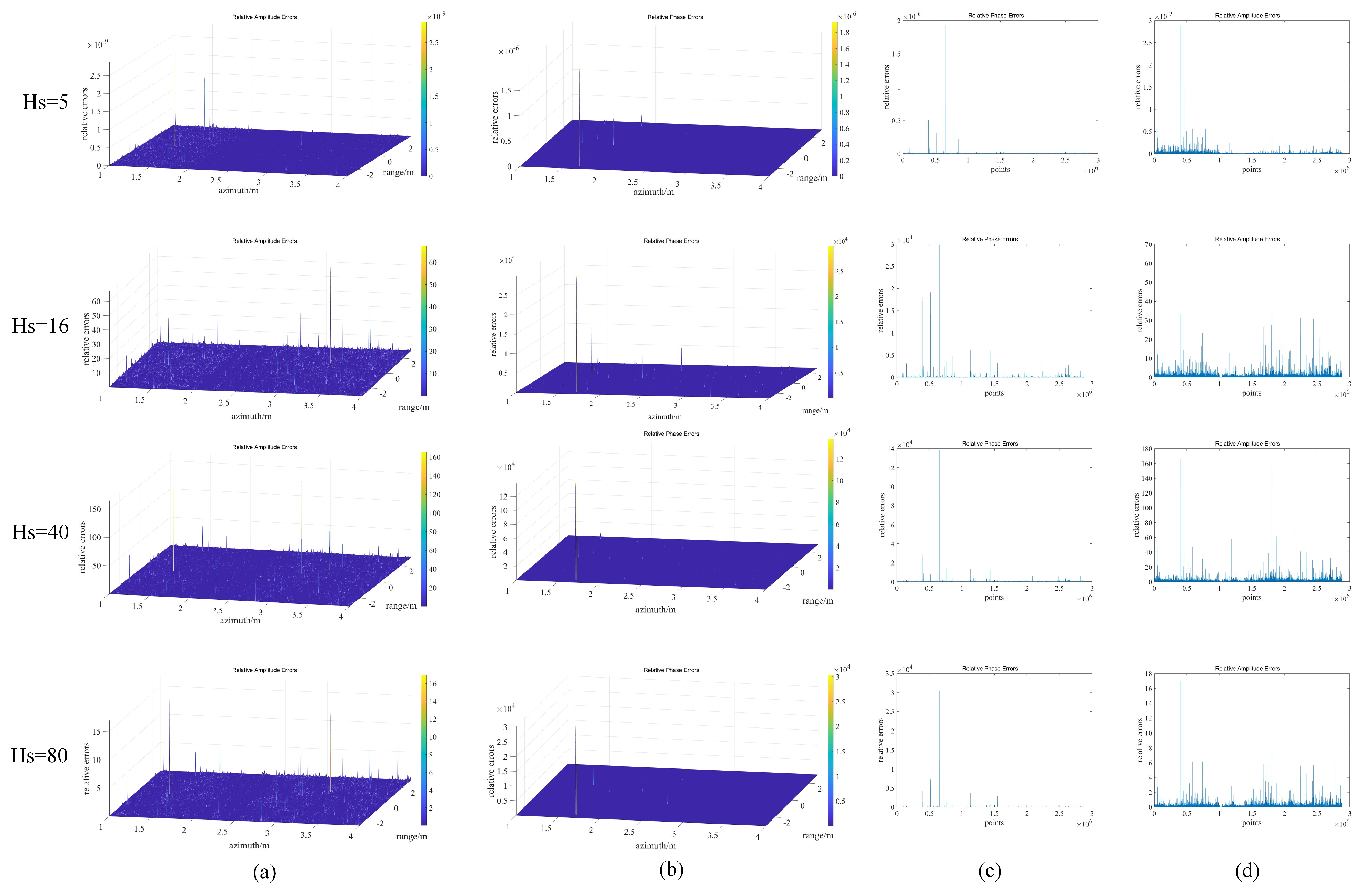
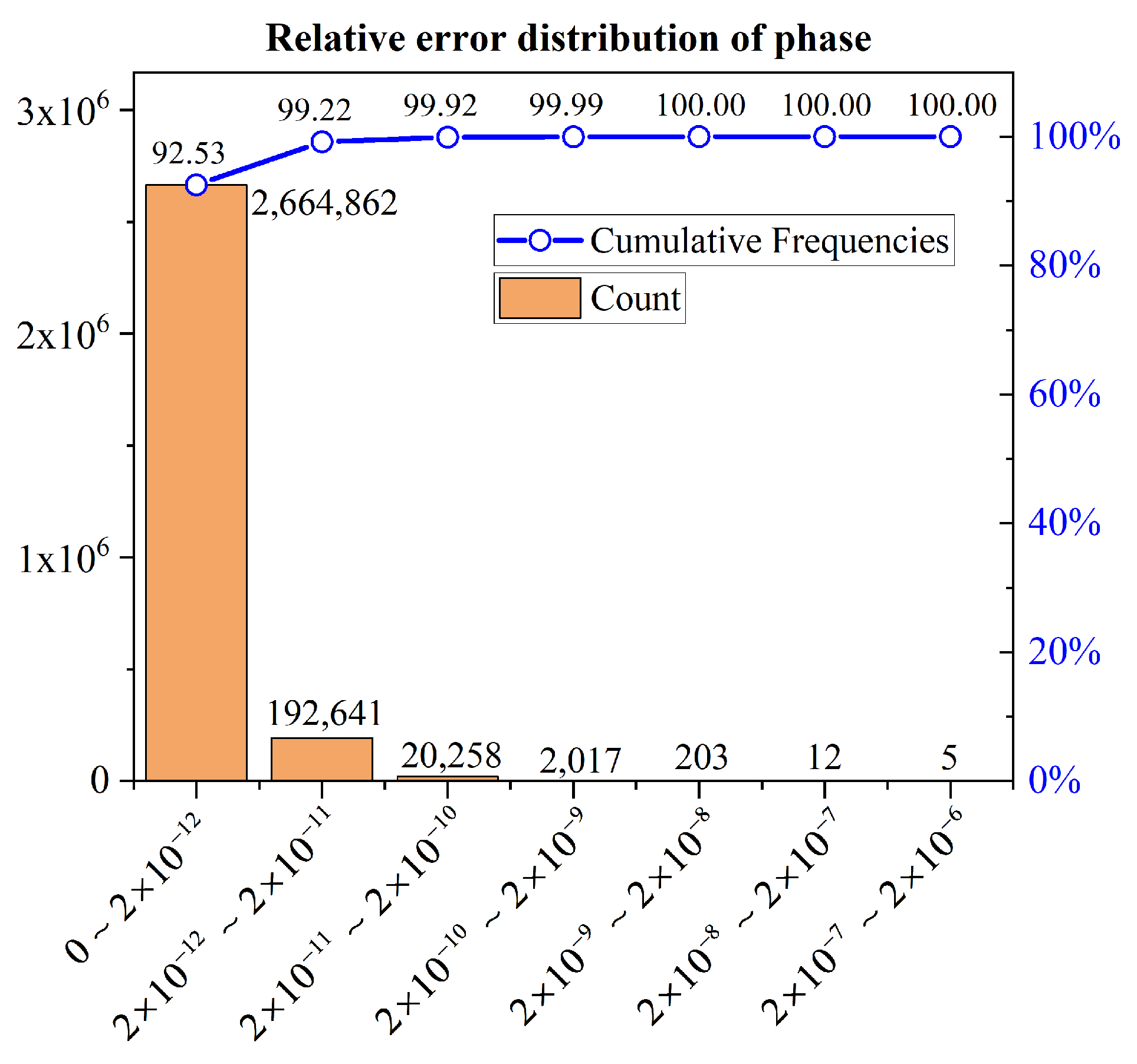
5.2. Experimental Results and Errors

As shown in Table 3, the traditional $\omega$KA has a runtime of 42,021.1 ms, while the real-time imaging scheme has a runtime of 1128.71 ms, resulting in a speed-up ratio of 37.23. As shown in

Table 4. Performance comparison of different interpolation methods.

	Traditional Interpolation Methods	Dynamic Parallel			Group-Nstream Mode	Fthread-Group- Nstream Mode
		One-Layer Nested Interpolation	Two-Layer Nested Interpolation	Three-Layer Nested Interpolation
Running time	29,070.4	7960.81 ms	1017.64 ms	timeout	571.863 ms	557.582 ms
Time complexity	$O(Na\times N{r}^2)$	$O(Na\times Nr)$	$O\left(Nr\right)$	$O\left(1\right)$	${\displaystyle \frac{Na\times Nr}{Ns}}$	${\displaystyle \frac{Na\times Nr}{Ns\times Hs}}$
Speed-up	/	3.65	28.57	/	50.83	52.14

, the traditional interpolation method has a runtime of 29,070.4 ms, which has the highest complexity. The three-layer nested interpolation has the lowest complexity, but its synchronization and dependency relationships are too complex to achieve a speed-up effect. The two-layer nested interpolation demonstrates the concurrency of the GPU through multi-level kernel functions, resulting in lower complexity and significant acceleration. However, it still needs to maintain synchronization and dependency relationships between the upper and lower layers of nesting. The $Group$-$Nstream$ mode is a further optimization of the two-layer nested interpolation, and it sacrifices some parallelism to achieve higher performance, with a runtime of 571.863 ms. Compared to the traditional interpolation method, the speedup of the $Group$-$Nstream$ mode can reach 50.83. The $Fthread$-$Group$-$Nstream$ mode employs a hybrid of CUDA and OpenMP, utilizing the CPU’s multi-core parallel capability to perform more fine-grained parallel computation in the $Group$-$Nstream$ mode, it has an execution time of 557.582 ms and a complexity of $\left(Na\times Nr\right)/\phantom{\left(Na\times Nr\right)\left(Ns\times Hs\right)}\left(Ns\times Hs\right)$.

Figure 14 and Figure 15 display the Pareto charts of the amplitude relative error and phase relative error in the $Fthread$-$Group$-$Nstream$ processing mode. It is evident that 93.45% of the pixel points have a relative error of the amplitude within $3\times {10}^{-14}\sim 3\times {10}^{-12}$, while 92.53% of the pixel points have a relative error of the phase within $0\sim 3\times {10}^{-12}$, indicating that the $Fthread$-$Group$-$Nstream$ mode achieves high precision.

In summary, the experimental results have verified that this method can effectively improve the performance of the imaging system. The $Fthread$-$Group$-$Nstream$ interpolation scheme achieved an acceleration ratio of 52.14, indicating that the efficiency of residual range migration correction, residual secondary range compression, and residual azimuth compression has been increased by 52.14 times. This significantly reduces the time cost and implementation complexity of three-dimensional interpolation. The overall acceleration ratio of the imaging scheme is 37.23, meaning that the efficiency of the imaging system in processing the echo data has increased by 37.23 times. As a result, the imaging system can accommodate higher data acquisition rates, enabling real-time data transmission and processing. This allows for the quick and accurate monitoring of deformable bodies, providing early warnings before geological disasters and the collapse of human-made structures, thereby preventing significant loss of life and property. Figure 16 depicts a rapid imaging image of a simulated sandbox. The proposed method not only exhibits good real-time performance but also delivers excellent imaging results with high precision.

6. Conclusions

This paper proposes a real-time imaging scheme different from traditional imaging algorithms, utilizing parallel processing and algorithm architecture. The proposed method achieves the efficient computation of parameter generation, zero-padding, one-dimensional and two-dimensional Fourier transforms, Stolt interpolation, and other operations, enabling real-time and high-precision data processing. This scheme is not only applicable to synthetic aperture radar (SAR); by adjusting the range equation, it can also be applied to synthetic aperture sonar (SAS) and synthetic aperture ultrasound imaging systems. The study draws the following main conclusions.

• Dynamic parallelism with multilayer kernel concurrency effectively achieves the rapid processing of three-dimensional signals. Three-layer nested interpolation has complex dependency and synchronization relationships, providing no acceleration effect. One-layer nested interpolation lacks sufficient depth, resulting in minimal acceleration. Two-layer nested interpolation demonstrates good parallelism and lower algorithm complexity.
• To further reduce the dependency and synchronization relationships between the upper and lower layers of two-layer nested interpolation, the $Group$-$Nstream$ model replaces the outermost layer of multiple threads in the two-layer nested interpolation with multiple non-blocking streams, reducing the impact of nested depth on algorithm performance in dynamic parallelism.
• The $Fthread$-$Group$-$Nstream$ processing model leverages the multi-core parallel capabilities of the CPU for finer-grained parallel computation of the $Group$-$Nstream$ model, addressing the issue of serial execution within $Group$s through hybrid programming with CUDA and OpenMP.
• The effectiveness and accuracy of the proposed method were verified through on-site experiments using a W-band GB-SAR system. The speed-up ratio of the imaging algorithm in this scheme is 37.23, with the interpolation part, which has a high computational load, achieving a speed-up ratio of up to 52.14. The relative amplitude and phase errors are close to 0.

References

1. Del Ventisette, C.; Intrieri, E.; Luzi, G.; Casagli, N.; Fanti, R.; Leva, D. Using ground based radar interferometry during emergency: The case of the A3 motorway (Calabria Region, Italy) threatened by a landslide. Nat. Hazards Earth Syst. Sci. 2011, 11, 2483–2495. [Google Scholar] [CrossRef]
2. Liu, B.; He, K.; Han, M.; Hu, X.; Ma, G.; Wu, M. Application of UAV and GB-SAR in Mechanism Research and Monitoring of Zhonghaicun Landslide in Southwest China. Remote Sens. 2021, 13, 1653. [Google Scholar] [CrossRef]
3. Wang, Y.; Song, Q.; Wang, J.; Yu, H. Airport Runway Foreign Object Debris Detection System Based on Arc-Scanning SAR Technology. IEEE Trans. Geosci. Remote Sens. 2022, 60, 1–16. [Google Scholar] [CrossRef]
4. Brown, S.; Quegan, S.; Morrison, K.; Bennett, J.; Cookmartin, G. High-resolution measurements of scattering in wheat canopies-implications for crop parameter retrieval. IEEE Trans. Geosci. Remote Sens. 2003, 41, 1602–1610. [Google Scholar] [CrossRef]
5. Xiang, X.; Chen, C.; Wang, H.; Lu, H.; Zhang, H.; Chen, J. A real-time processing method for GB-SAR monitoring data by using the dynamic Kalman filter based on the PS network. Landslides 2023, 20, 1639–1655. [Google Scholar] [CrossRef]
6. Jakovljevic, M.; Michaelides, R.; Biondi, E.; Hyun, D.; Zebker, H.A.; Dahl, J.J. Adaptation of Range-Doppler Algorithm for Efficient Beamforming of Monostatic and Multistatic Ultrasound Signals. IEEE Trans. Ultrason. Ferroelectr. Freq. Control 2022, 69, 3165–3178. [Google Scholar] [CrossRef]
7. Ma, M.; Tang, J.; Wu, H.; Zhang, P.; Ning, M. CZT Algorithm for the Doppler Scale Signal Model of Multireceiver SAS Based on Shear Theorem. IEEE Trans. Geosci. Remote Sens. 2023, 61, 1–12. [Google Scholar] [CrossRef]
8. Li, Z.; Zhang, X.; Yang, Q.; Xiao, Y.; An, H.; Yang, H.; Wu, J.; Yang, J. Hybrid SAR-ISAR Image Formation via Joint FrFT-WVD Processing for BFSAR Ship Target High-Resolution Imaging. IEEE Trans. Geosci. Remote Sens. 2022, 60, 1–13. [Google Scholar] [CrossRef]
9. Wang, H.; Chen, X.; Sun, J. FMCW SAR Imaging Algorithm of Sliding Spotlight Mode. IEEE Geosci. Remote Sens. Lett. 2022, 19, 1–5. [Google Scholar] [CrossRef]
10. Lin, J.Z.; Chen, P.T.; Chin, H.Y.; Tsai, P.Y.; Lee, S.Y. Design and Implementation of a Real-Time Imaging Processor for Spaceborne Synthetic Aperture Radar with Configurability. IEEE Trans. Very Large Scale Integr. Syst. 2024, 32, 669–681. [Google Scholar] [CrossRef]
11. Bi, H.; Wang, J.; Bi, G. Wavenumber Domain Algorithm-Based FMCW SAR Sparse Imaging. IEEE Trans. Geosci. Remote Sens. 2019, 57, 7466–7475. [Google Scholar] [CrossRef]
12. Zhou, J.; Zhu, R.; Jiang, G.; Zhao, L.; Cheng, B. A Precise Wavenumber Domain Algorithm for Near Range Microwave Imaging by Cross MIMO Array. IEEE Trans. Microw. Theory Tech. 2019, 67, 1316–1326. [Google Scholar] [CrossRef]
13. Xu, G.; Xing, M.; Zhang, L.; Bao, Z. Robust Autofocusing Approach for Highly Squinted SAR Imagery Using the Extended Wavenumber Algorithm. IEEE Trans. Geosci. Remote Sens. 2013, 51, 5031–5046. [Google Scholar] [CrossRef]
14. Zhang, L.; Sheng, J.; Xing, M.; Qiao, Z.; Xiong, T.; Bao, Z. Wavenumber-Domain Autofocusing for Highly Squinted UAV SAR Imagery. IEEE Sens. J. 2012, 12, 1574–1588. [Google Scholar] [CrossRef]
15. Chen, Y.; Xiong, Z.; Kong, Q.; Ma, X.; Chen, M.; Lu, C. Circular statistics vector for improving coherent plane wave compounding image in Fourier domain. Ultrasonics 2023, 128, 106856. [Google Scholar] [CrossRef]
16. Waller, E.H.; Keil, A.; Friederich, F. Quantum range-migration-algorithm for synthetic aperture radar applications. Sci. Rep. 2023, 13, 11436. [Google Scholar] [CrossRef]
17. Chen, X.; Wang, H.; Yang, Q.; Zeng, Y.; Deng, B. An Efficient mmW Frequency-Domain Imaging Algorithm for Near-Field Scanning 1-D SIMO/MIMO Array. IEEE Trans. Instrum. Meas. 2022, 71, 1–12. [Google Scholar] [CrossRef]
18. Garcia, D.; Tarnec, L.L.; Muth, S.; Montagnon, E.; Porée, J.; Cloutier, G. Stolt’s f-k migration for plane wave ultrasound imaging. IEEE Trans. Ultrason. Ferroelectr. Freq. Control 2013, 60, 1853–1867. [Google Scholar] [CrossRef]
19. Skjelvareid, M.H.; Olofsson, T.; Birkelund, Y.; Larsen, Y. Synthetic aperture focusing of ultrasonic data from multilayered media using an omega-K algorithm. IEEE Trans. Ultrason. Ferroelectr. Freq. Control 2011, 58, 1037–1048. [Google Scholar] [CrossRef]
20. Xiong, Y.; Liang, B.; Yu, H.; Chen, J.; Jin, Y.; Xing, M. Processing of Bistatic SAR Data with Nonlinear Trajectory Using a Controlled-SVD Algorithm. IEEE J. Sel. Top. Appl. Earth Obs. Remote Sens. 2021, 14, 5750–5759. [Google Scholar] [CrossRef]
21. Zaghiyan, M.R.; Eslamian, S.; Gohari, A.; Ebrahimi, M.S. Temporal correction of irregular observed intervals of groundwater level series using interpolation techniques. Theor. Appl. Climatol. 2021, 145, 1027–1037. [Google Scholar] [CrossRef]
22. Skouroliakou, V.; Molaei, A.M.; Fusco, V.; Yurduseven, O. Fourier-based Radar Processing for Multistatic Millimetre-wave Imaging with Sparse Apertures. In Proceedings of the 2022 16th European Conference on Antennas and Propagation (EuCAP), Madrid, Spain, 27 March–1 April 2022; pp. 1–5. [Google Scholar] [CrossRef]
23. Wang, L.; Ai, Z.; Shi, J.; Wang, J.; Zhang, X.; Yang, J. Low Computational Complexity SAR Imaging Algorithm for Ship Monitoring via 2-D Band-Limited Sparse Fourier Transform. IEEE Sens. J. 2024, 24, 13326–13342. [Google Scholar] [CrossRef]
24. Tan, Y.; Lai, T.; Ou, P.; Dan, Q.; Huang, H. Subaperture Real-time Imaging Algorithm Based on GPU. In Proceedings of the EEI 2022; 4th International Conference on Electronic Engineering and Informatics, Guiyang, China, 24–26 June 2022; pp. 1–9. [Google Scholar]
25. Cumming, I.G.; Wong, F.H. Digital processing of synthetic aperture radar data. Artech House 2005, 1, 108–110. [Google Scholar]
26. Molaei, A.M.; Fromenteze, T.; Skouroliakou, V.; Hoang, T.V.; Kumar, R.; Fusco, V.; Yurduseven, O. Development of Fast Fourier-Compatible Image Reconstruction for 3D Near-Field Bistatic Microwave Imaging with Dynamic Metasurface Antennas. IEEE Trans. Veh. Technol. 2022, 71, 13077–13090. [Google Scholar] [CrossRef]
27. Zhang, F.; Hu, C.; Li, W.; Hu, W.; Wang, P.; Li, H.C. A Deep Collaborative Computing Based SAR Raw Data Simulation on Multiple CPU/GPU Platform. IEEE J. Sel. Top. Appl. Earth Obs. Remote Sens. 2017, 10, 387–399. [Google Scholar] [CrossRef]
28. Wang, Y.; Li, W.; Liu, T.; Zhou, L.; Wang, B.; Fan, Z.; Ye, X.; Fan, D.; Ding, C. Characterization and Implementation of Radar System Applications on a Reconfigurable Dataflow Architecture. IEEE Comput. Archit. Lett. 2022, 21, 121–124. [Google Scholar] [CrossRef]
29. Guo, Y.; Davy, A.; Facciolo, G.; Morel, J.M.; Jin, Q. Fast, Nonlocal and Neural: A Lightweight High Quality Solution to Image Denoising. IEEE Signal Process. Lett. 2021, 28, 1515–1519. [Google Scholar] [CrossRef]
30. Romano, D.; Lapegna, M.; Mele, V.; Laccetti, G. Designing a GPU-parallel algorithm for raw SAR data compression: A focus on parallel performance estimation. Future Gener. Comput. Syst. 2020, 112, 695–708. [Google Scholar] [CrossRef]
31. Imperatore, P.; Pepe, A.; Sansosti, E. High Performance Computing in Satellite SAR Interferometry: A Critical Perspective. Remote Sens. 2021, 13, 4756. [Google Scholar] [CrossRef]
32. Zhang, F.; Hu, C.; Li, W.; Hu, W.; Li, H.C. Accelerating Time-Domain SAR Raw Data Simulation for Large Areas Using Multi-GPUs. IEEE J. Sel. Top. Appl. Earth Obs. Remote Sens. 2014, 7, 3956–3966. [Google Scholar] [CrossRef]
33. Chen, Y.; Feng, W.; Ranftl, R.; Qiao, H.; Pock, T. A Higher-Order MRF Based Variational Model for Multiplicative Noise Reduction. IEEE Signal Process. Lett. 2014, 21, 1370–1374. [Google Scholar] [CrossRef]
34. Jin, H.; Chen, J. An efficient wavenumber algorithm towards real-time ultrasonic full-matrix imaging of multi-layered medium. Mech. Syst. Signal Process. 2021, 149, 107149. [Google Scholar] [CrossRef]
35. Yu, B.; Jin, H.; Mei, Y.; Chen, J.; Wu, E.; Yang, K. 3-D ultrasonic image reconstruction in frequency domain using a virtual transducer model. Ultrasonics 2022, 118, 106573. [Google Scholar] [CrossRef] [PubMed]
36. Hernández-Burgos, S.; Gibert, F.; Broquetas, A.; Kleinherenbrink, M.; De la Cruz, A.F.; Gómez-Olivé, A.; García-Mondéjar, A.; i Aparici, M.R. A Fully Focused SAR Omega-K Closed-Form Algorithm for the Sentinel-6 Radar Altimeter: Methodology and Applications. IEEE Trans. Geosci. Remote Sens. 2024, 62, 1–16. [Google Scholar] [CrossRef]
37. Shi, H.; Zhang, L.; Liu, D.; Yang, T.; Guo, J. SAR Imaging Method for Moving Targets Based on Omega-k and Fourier Ptychographic Microscopy. IEEE Geosci. Remote Sens. Lett. 2022, 19, 1–5. [Google Scholar] [CrossRef]
38. Sun, G.C.; Liu, Y.; Xiang, J.; Liu, W.; Xing, M.; Chen, J. Spaceborne Synthetic Aperture Radar Imaging Algorithms: An overview. IEEE Geosci. Remote Sens. Mag. 2022, 10, 161–184. [Google Scholar] [CrossRef]
39. Moreira, A. Real-time synthetic aperture radar (SAR) processing with a new subaperture approach. IEEE Trans. Geosci. Remote Sens. 1992, 30, 714–722. [Google Scholar] [CrossRef]
40. Li, Z.; Wang, J.; Liu, Q.H. Interpolation-Free Stolt Mapping for SAR Imaging. IEEE Geosci. Remote Sens. Lett. 2014, 11, 926–929. [Google Scholar] [CrossRef]
41. Meng, Y.; Lin, C.; Qing, A.; Nikolova, N.K. Accelerated Holographic Imaging With Range Stacking for Linear Frequency Modulation Radar. IEEE Trans. Microw. Theory Tech. 2022, 70, 1630–1638. [Google Scholar] [CrossRef]
42. Cheng, J.; Grossman, M.; McKercher, T. Professional CUDA c Programming; John Wiley & Sons: Hoboken, NJ, USA, 2014. [Google Scholar]
43. Chandra, R. Parallel Programming in OpenMP; Morgan Kaufmann: Burlington, MA, USA, 2001. [Google Scholar]
44. Huber, J.; Cornelius, M.; Georgakoudis, G.; Tian, S.; Diaz, J.M.M.; Dinel, K.; Chapman, B.; Doerfert, J. Efficient Execution of OpenMP on GPUs. In Proceedings of the 2022 IEEE/ACM International Symposium on Code Generation and Optimization (CGO), Seoul, Republic of Korea, 2–6 April 2022; pp. 41–52. [Google Scholar] [CrossRef]
45. Aldinucci, M.; Cesare, V.; Colonnelli, I.; Martinelli, A.R.; Mittone, G.; Cantalupo, B.; Cavazzoni, C.; Drocco, M. Practical parallelization of scientific applications with OpenMP, OpenACC and MPI. J. Parallel Distrib. Comput. 2021, 157, 13–29. [Google Scholar] [CrossRef]
46. Hoffmann, R.B.; Löff, J.; Griebler, D.; Fernandes, L.G. OpenMP as runtime for providing high-level stream parallelism on multi-cores. J. Supercomput. 2022, 78, 7655–7676. [Google Scholar] [CrossRef]
47. Daleiden, P.; Stefik, A.; Uesbeck, P.M. GPU programming productivity in different abstraction paradigms: A randomized controlled trial comparing CUDA and thrust. ACM Trans. Comput. Educ. (TOCE) 2020, 20, 1–27. [Google Scholar] [CrossRef]
48. Ansorge, R. Programming in Parallel with CUDA: A Practical Guide; Cambridge University Press: Cambridge, UK, 2022. [Google Scholar]
Figure 1. Working schematic diagram of real-time imaging scheme.
Electronics 13 03138 g001
Figure 2. Regions of data protrusion and discard in Stolt mapping.
Electronics 13 03138 g002
Figure 3. Generating relevant parameters and functions through non-blocking stream.
Electronics 13 03138 g003
Figure 4. One-layer nested interpolation.
Electronics 13 03138 g004
Figure 5. Two-layer nested interpolation.
Electronics 13 03138 g005
Figure 6. Three-layer nested interpolation.
Electronics 13 03138 g006
Figure 7. The  i n t e r p 2 _ G P U  kernel function.
Electronics 13 03138 g007
Figure 8. G r o u p - N s t r e a m  processing mode schematic diagram.
Electronics 13 03138 g008
Figure 9. The Fork–Join parallel execution model used by OpenMP.
Electronics 13 03138 g009
Figure 10. f t h r e a - G r o u p - N s t r e a m  processing mode. (a G r o u p  parallel execution, (b) diagram of subtask partitioning and indexing.
Electronics 13 03138 g010
Figure 11. The impact of the number of streams on algorithm performance and interpolation time.
Electronics 13 03138 g011
Figure 12. Subtasks are executed in parallel in  G r o u p - S t r e a m  mode.
Electronics 13 03138 g012
Figure 13. Imaging errors for different values of  H s . (a) Relative amplitude error of the imaging scene, (b) relative phase error of the imaging scene, (c) scatter plot of relative phase error, (d) scatter plot of relative amplitude error.
Electronics 13 03138 g013
Figure 14. Pareto chart of relative amplitude error distribution.
Electronics 13 03138 g014
Figure 15. Pareto chart of relative phase error distribution.
Electronics 13 03138 g015
Figure 16. Imaging results. (a) is the original image, (b) is a normalized image, (c) is the azimuth section diagram, and (d) is the range section diagram.
Electronics 13 03138 g016