
Generated or Not Generated (GNG): The Importance of Background in the Detection of Fake Images

 , , ,
, , ,  , and
, and
Abstract
1. Introduction
2. Materials and Methods
2.1. Datasets
2.2. StyleGAN Family
2.3. DeepLabV3+
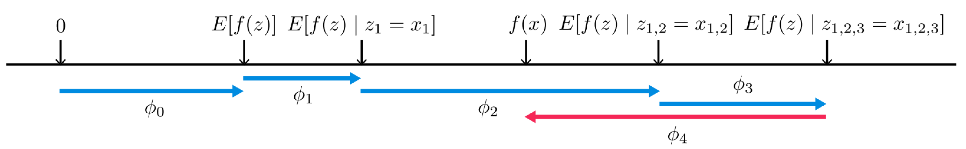
2.4. SHAP
2.5. Experimental Setup
3. Results and Discussion
4. Conclusions
Supplementary Materials
Author Contributions
Funding
Data Availability Statement
Acknowledgments
Conflicts of Interest
Abbreviations
| MDPI | Multidisciplinary Digital Publishing Institute |
| AI | Artificial Intelligence |
| ML | Machine Learning |
| DL | Deep Learning |
| GNG | Generated or Not Generated |
| GAN | Generative Adversarial Network |
| CNN | Convolutional Neural Network |
| MLP | Multilayer Perceptron |
| SHAP | SHapley Additive exPlanation |
| ArtiFact | Artificial and Factual |
| FFHQ | Flickr-Faces-HQ |
| SPP | Spatial Pyramid Pooling |
| ASPP | Atrous Spatial Pyramid Pooling |
| TP | True Positive |
| TN | True Negative |
| FP | False Positive |
| FN | False Negative |
References
- Karras, T.; Laine, S.; Aila, T. A style-based generator architecture for generative adversarial networks. In Proceedings of the IEEE/CVF Conference on Computer Vision and Pattern Recognition, Long Beach, CA, USA, 15–20 June 2019; pp. 4401–4410. [Google Scholar]
- Rombach, R.; Blattmann, A.; Lorenz, D.; Esser, P.; Ommer, B. High-resolution image synthesis with latent diffusion models. In Proceedings of the IEEE/CVF Conference on Computer Vision and Pattern Recognition, New Orleans, LA, USA, 18–24 June 2022; pp. 10684–10695. [Google Scholar]
- LeCun, Y.; Bengio, Y.; Hinton, G. Deep learning. Nature 2015, 521, 436–444. [Google Scholar] [CrossRef]
- Yamashita, R.; Nishio, M.; Do, R.K.G.; Togashi, K. Convolutional neural networks: An overview and application in radiology. INsights Into Imaging 2018, 9, 611–629. [Google Scholar] [CrossRef]
- Li, Z.; Liu, F.; Yang, W.; Peng, S.; Zhou, J. A survey of convolutional neural networks: Analysis, applications, and prospects. IEEE Trans. Neural Netw. Learn. Syst. 2021, 33, 6999–7019. [Google Scholar] [CrossRef] [PubMed]
- LeCun, Y.; Boser, B.; Denker, J.S.; Henderson, D.; Howard, R.E.; Hubbard, W.; Jackel, L.D. Backpropagation applied to handwritten zip code recognition. Neural Comput. 1989, 1, 541–551. [Google Scholar] [CrossRef]
- LeCun, Y.; Bottou, L.; Bengio, Y.; Haffner, P. Gradient-based learning applied to document recognition. Proc. IEEE 1998, 86, 2278–2324. [Google Scholar] [CrossRef]
- Krizhevsky, A.; Sutskever, I.; Hinton, G.E. ImageNet classification with deep convolutional neural networks. Adv. Neural Inf. Process. Syst. 2012, 25, 1097–1105. [Google Scholar] [CrossRef]
- Girshick, R.; Donahue, J.; Darrell, T.; Malik, J. Rich feature hierarchies for accurate object detection and semantic segmentation. In Proceedings of the IEEE Conference on Computer Vision and Pattern Recognition, Columbus, OH, USA, 23–28 June 2014; pp. 580–587. [Google Scholar]
- Monaci, M.; Pancino, N.; Andreini, P.; Bonechi, S.; Bongini, P.; Rossi, A.; Ciano, G.; Giacomini, G.; Scarselli, F.; Bianchini, M.; et al. Deep Learning Techniques for Dragonfly Action Recognition. In Proceedings of the ICPRAM, Valletta, Malta, 22–24 February 2020; pp. 562–569. [Google Scholar]
- Pancino, N.; Graziani, C.; Lachi, V.; Sampoli, M.L.; Ștefǎnescu, E.; Bianchini, M.; Dimitri, G.M. A mixed statistical and machine learning approach for the analysis of multimodal trail making test data. Mathematics 2021, 9, 3159. [Google Scholar] [CrossRef]
- Landi, E.; Spinelli, F.; Intravaia, M.; Mugnaini, M.; Fort, A.; Bianchini, M.; Corradini, B.T.; Scarselli, F.; Tanfoni, M. A MobileNet Neural Network Model for Fault Diagnosis in Roller Bearings. In Proceedings of the 2023 IEEE International Instrumentation and Measurement Technology Conference (I2MTC), Kuala Lumpur, Malaysia, 22–25 May 2023; pp. 1–6. [Google Scholar] [CrossRef]
- Stefanescu, E.; Pancino, N.; Graziani, C.; Lachi, V.; Sampoli, M.; Dimitri, G.; Bargagli, A.; Zanca, D.; Bianchini, M.; Mureșanu, D.; et al. Blinking Rate Comparison Between Patients with Chronic Pain and Parkinson’s Disease. Eur. J. Neurol. 2022, 29, 669. [Google Scholar]
- Russo, V.; Lallo, E.; Munnia, A.; Spedicato, M.; Messerini, L.; D’Aurizio, R.; Ceroni, E.G.; Brunelli, G.; Galvano, A.; Russo, A.; et al. Artificial intelligence predictive models of response to cytotoxic chemotherapy alone or combined to targeted therapy for metastatic colorectal cancer patients: A systematic review and meta-analysis. Cancers 2022, 14, 4012. [Google Scholar] [CrossRef]
- Lee, S.; Lee, J.; Lee, K.M. V-net: End-to-end convolutional network for object detection. Expert Syst. Appl. 2017, 90, 295–304. [Google Scholar]
- Liang, J.; Li, N.; Sun, X.; Wang, X.; Liu, M.; Shi, J.; Huang, J.; Wang, D.Y. CIRL: Continuous imitation learning from human interaction with reinforcement learning in autonomous driving. IEEE Trans. Intell. Transp. Syst. 2018, 20, 4038–4052. [Google Scholar]
- Chen, T.; Liu, S.; Yang, X.; Shen, J.; Hu, X.; Yang, G. Deepdriving: Learning affordance for direct perception in autonomous driving. In Proceedings of the AAAI Conference on Artificial Intelligence, Austin, TX, USA, 25–30 January 2015; Volume 29, pp. 2722–2728. [Google Scholar]
- Bojarski, M.; Del Testa, D.; Dworakowski, D.; Firner, B.; Flepp, B.; Goyal, P.; Jackel, L.D.; Monfort, M.; Muller, U.; Zhang, J.; et al. End to end learning for self-driving cars. arXiv 2016, arXiv:1604.07316. [Google Scholar]
- Chen, L.C.; Zhu, Y.; Papandreou, G.; Schroff, F.; Adam, H. Encoder-decoder with atrous separable convolution for semantic image segmentation. In Proceedings of the European Conference on Computer Vision (ECCV), Munich, Germany, 8–14 September 2018; pp. 801–818. [Google Scholar]
- Chen, L.C.; Papandreou, G.; Kokkinos, I.; Murphy, K.; Yuille, A.L. Deeplab: Semantic image segmentation with deep convolutional nets, atrous convolution, and fully connected crfs. IEEE Trans. Pattern Anal. Mach. Intell. 2017, 40, 834–848. [Google Scholar] [CrossRef]
- Long, J.; Shelhamer, E.; Darrell, T. Fully convolutional networks for semantic segmentation. In Proceedings of the IEEE Conference on Computer Vision and Pattern Recognition, Boston, MA, USA, 7–12 June 2015; pp. 3431–3440. [Google Scholar]
- Andreini, P.; Pancino, N.; Costanti, F.; Eusepi, G.; Corradini, B.T. A Deep Learning approach for oocytes segmentation and analysis. In Proceedings of the ESANN, Bruges (Belgium) and Online Event, 5–7 October 2022. [Google Scholar]
- Radford, A.; Metz, L.; Chintala, S. Unsupervised Representation Learning with Deep Convolutional Generative Adversarial Networks. arXiv 2015, arXiv:1511.06434. [Google Scholar]
- Goodfellow, I.; Pouget-Abadie, J.; Mirza, M.; Xu, B.; Warde-Farley, D.; Ozair, S.; Courville, A.; Bengio, Y. Generative adversarial nets. Adv. Neural Inf. Process. Syst. 2014, 27, 2672–2680. [Google Scholar]
- Karras, T.; Laine, S.; Aittala, M.; Hellsten, J.; Lehtinen, J.; Aila, T. Analyzing and improving the image quality of stylegan. In Proceedings of the IEEE/CVF Conference on Computer Vision and Pattern Recognition, Seattle, WA, USA, 13–19 June 2020; pp. 8110–8119. [Google Scholar]
- Karras, T.; Aittala, M.; Laine, S.; Härkönen, E.; Hellsten, J.; Lehtinen, J.; Aila, T. Alias-free generative adversarial networks. Adv. Neural Inf. Process. Syst. 2021, 34, 852–863. [Google Scholar]
- Brock, A.; Donahue, J.; Simonyan, K. Large Scale GAN Training for High Fidelity Natural Image Synthesis. arXiv 2019, arXiv:1809.11096. [Google Scholar]
- Wang, X.; Guo, H.; Hu, S.; Chang, M.C.; Lyu, S. Gan-generated faces detection: A survey and new perspectives. ECAI 2023, 2023, 2533–2542. [Google Scholar]
- Le, T.N.; Nguyen, H.H.; Yamagishi, J.; Echizen, I. OpenForensics: Large-Scale Challenging Dataset For Multi-Face Forgery Detection And Segmentation In-The-Wild. In Proceedings of the 2021 IEEE/CVF International Conference on Computer Vision (ICCV), Montreal, BC, Canada, 11–17 October 2021; pp. 10097–10107. [Google Scholar] [CrossRef]
- Simonyan, K. Very deep convolutional networks for large-scale image recognition. arXiv 2015, arXiv:1409.1556. [Google Scholar]
- Gu, Q.; Chen, S.; Yao, T.; Chen, Y.; Ding, S.; Yi, R. Exploiting fine-grained face forgery clues via progressive enhancement learning. In Proceedings of the AAAI Conference on Artificial Intelligence, Virtual, 22 February–1 March 2022; Volume 36, pp. 735–743. [Google Scholar]
- Qian, Y.; Yin, G.; Sheng, L.; Chen, Z.; Shao, J. Thinking in frequency: Face forgery detection by mining frequency-aware clues. In Proceedings of the European Conference on Computer Vision, Glasgow, UK, 23–28 August 2020; Springer: Berlin/Heidelberg, Germany, 2020; pp. 86–103. [Google Scholar]
- Songsri-in, K.; Zafeiriou, S. Complement Face Forensic Detection and Localization with FacialLandmarks. arXiv 2019, arXiv:1910.05455. [Google Scholar]
- Nadimpalli, A.V.; Rattani, A. Facial Forgery-Based Deepfake Detection Using Fine-Grained Features. In Proceedings of the 2023 International Conference on Machine Learning and Applications (ICMLA), Jacksonville, FL, USA, 15–17 December 2023; pp. 2174–2181. [Google Scholar] [CrossRef]
- Liu, Z.; Qi, X.; Torr, P.H. Global texture enhancement for fake face detection in the wild. In Proceedings of the IEEE/CVF Conference on Computer Vision and Pattern Recognition, Seattle, WA, USA, 13–19 June 2020; pp. 8057–8066. [Google Scholar]
- Chen, B.; Liu, X.; Zheng, Y.; Zhao, G.; Shi, Y.Q. A Robust GAN-Generated Face Detection Method Based on Dual-Color Spaces and an Improved Xception. IEEE Trans. Circuits Syst. Video Technol. 2022, 32, 3527–3538. [Google Scholar] [CrossRef]
- Wang, R.; Juefei-Xu, F.; Ma, L.; Xie, X.; Huang, Y.; Wang, J.; Liu, Y. FakeSpotter: A simple yet robust baseline for spotting AI-synthesized fake faces. In Proceedings of the P Twenty-Ninth International Joint Conference on Artificial Intelligence (IJCAI2020), Yokohama, Japan, 7–15 January 2021. [Google Scholar]
- Liang, B.; Wang, Z.; Huang, B.; Zou, Q.; Wang, Q.; Liang, J. Depth map guided triplet network for deepfake face detection. Neural Netw. 2023, 159, 34–42. [Google Scholar] [CrossRef]
- Howard, A.; Sandler, M.; Chen, B.; Wang, W.; Chen, L.C.; Tan, M.; Chu, G.; Vasudevan, V.; Zhu, Y.; Pang, R.; et al. Searching for MobileNetV3. In Proceedings of the 2019 IEEE/CVF International Conference on Computer Vision (ICCV), Seoul, Korea, 27 October–2 November 2019; pp. 1314–1324. [Google Scholar] [CrossRef]
- Lundberg, S.M.; Lee, S.I. A unified approach to interpreting model predictions. Adv. Neural Inf. Process. Syst. 2017, 30, 4766–4775. [Google Scholar]
- Mut1ny, J.D. Face/Head Segmentation Dataset Commercial Purpose Edition; Spriaeastraat: Den Haag, Netherlands, 2024. [Google Scholar]
- Hassani, A.; Shair, Z.E.; Ud Duala Refat, R.; Malik, H. Distilling Facial Knowledge with Teacher-Tasks: Semantic-Segmentation-Features For Pose-Invariant Face-Recognition. In Proceedings of the 2022 IEEE International Conference on Image Processing (ICIP), Bordeaux, France, 16–19 October 2022; pp. 741–745. [Google Scholar] [CrossRef]
- Reimann, M.; Klingbeil, M.; Pasewaldt, S.; Semmo, A.; Trapp, M.; Döllner, J. Locally controllable neural style transfer on mobile devices. Vis. Comput. 2019, 35, 1531–1547. [Google Scholar] [CrossRef]
- Khoshnevisan, E.; Hassanpour, H.; AlyanNezhadi, M.M. Face recognition based on general structure and angular face elements. Multimed. Tools Appl. 2024, 1–19. [Google Scholar] [CrossRef]
- Mut1ny, J.D. Face/Head Segmentation Dataset Community Edition; Spriaeastraat: Den Haag, Netherlands, 2024. [Google Scholar]
- Rahman, M.A.; Paul, B.; Sarker, N.H.; Hakim, Z.I.A.; Fattah, S.A. Artifact: A large-scale dataset with artificial and factual images for generalizable and robust synthetic image detection. In Proceedings of the 2023 IEEE International Conference on Image Processing (ICIP), IEEE, Kuala Lumpur, Malaysia, 8–11 October 2023; pp. 2200–2204. [Google Scholar]
- Wang, Z.; Zheng, H.; He, P.; Chen, W.; Zhou, M. Diffusion-GAN: Training GANs with Diffusion. arXiv 2023, arXiv:2206.02262. [Google Scholar]
- Zhu, J.Y.; Park, T.; Isola, P.; Efros, A.A. Unpaired Image-to-Image Translation using Cycle-Consistent Adversarial Networks. arXiv 2020, arXiv:1703.10593. [Google Scholar]
- Esser, P.; Rombach, R.; Ommer, B. Taming Transformers for High-Resolution Image Synthesis. arXiv 2020, arXiv:2012.09841. [Google Scholar]
- Xia, W.; Yang, Y.; Xue, J.H.; Wu, B. Tedigan: Text-guided diverse face image generation and manipulation. In Proceedings of the IEEE/CVF Conference on Computer Vision and Pattern Recognition, Nashville, TN, USA, 20–25 June 2021; pp. 2256–2265. [Google Scholar]
- Liu, Z.; Luo, P.; Wang, X.; Tang, X. Deep Learning Face Attributes in the Wild. In Proceedings of the International Conference on Computer Vision (ICCV), Santiago, Chile, 7–13 December 2015. [Google Scholar]
- Lin, T.Y.; Maire, M.; Belongie, S.; Hays, J.; Perona, P.; Ramanan, D.; Dollár, P.; Zitnick, C.L. Microsoft COCO: Common Objects in Context. In Proceedings of the Computer Vision—ECCV 2014, Zurich, Switzerland, 6–12 September 2014; Fleet, D., Pajdla, T., Schiele, B., Tuytelaars, T., Eds.; Springer: Cham, Switzerland, 2014; pp. 740–755. [Google Scholar]
- Karras, T.; Aila, T.; Laine, S.; Lehtinen, J. Progressive Growing of GANs for Improved Quality, Stability, and Variation. In Proceedings of the International Conference on Learning Representations, Vancouver, BC, Canada, 30 April–3 May 2018. [Google Scholar]
- Huang, X.; Belongie, S. Arbitrary style transfer in real-time with adaptive instance normalization. In Proceedings of the IEEE International Conference on Computer Vision, Venice, Italy, 22–29 October 2017; pp. 1501–1510. [Google Scholar]
- He, K.; Zhang, X.; Ren, S.; Sun, J. Spatial pyramid pooling in deep convolutional networks for visual recognition. IEEE Trans. Pattern Anal. Mach. Intell. 2015, 37, 1904–1916. [Google Scholar] [CrossRef]
- Shapley, L.S. 17. A Value for n-Person Games. In Contributions to the Theory of Games (AM-28), Volume II; Kuhn, H.W., Tucker, A.W., Eds.; Princeton University Press: Princeton, NJ, USA, 1953; pp. 307–318. [Google Scholar] [CrossRef]
- Schmeidler, D. The Nucleolus of a Characteristic Function Game. SIAM J. Appl. Math. 1969, 17, 1163–1170. [Google Scholar] [CrossRef]
- Shapley, L.S.; Shubik, M. A Method for Evaluating the Distribution of Power in a Committee System. Am. Political Sci. Rev. 1954, 48, 787–792. [Google Scholar] [CrossRef]
- Roth, A.E. Introduction to the Shapley value. In The Shapley Value: Essays in Honor of Lloyd S. Shapley; Roth, A.E., Ed.; Cambridge University Press: Cambridge, UK, 1988; pp. 1–28. [Google Scholar]
- Ribeiro, M.T.; Singh, S.; Guestrin, C. “Why should i trust you?” Explaining the predictions of any classifier. In Proceedings of the 22nd ACM SIGKDD International Conference on Knowledge Discovery and Data Mining, San Francisco, CA, USA, 13–17 August 2016; pp. 1135–1144. [Google Scholar]
- Shrikumar, A.; Greenside, P.; Kundaje, A. Learning important features through propagating activation differences. In Proceedings of the International Conference on Machine Learning. PMLR, Sydney, Australia, 6–11 August 2017; pp. 3145–3153. [Google Scholar]
- Bach, S.; Binder, A.; Montavon, G.; Klauschen, F.; Müller, K.R.; Samek, W. On pixel-wise explanations for non-linear classifier decisions by layer-wise relevance propagation. PLoS ONE 2015, 10, e0130140. [Google Scholar] [CrossRef] [PubMed]
- Lipovetsky, S.; Conklin, M. Analysis of regression in game theory approach. Appl. Stoch. Model. Bus. Ind. 2001, 17, 319–330. [Google Scholar] [CrossRef]
- Štrumbelj, E.; Kononenko, I. Explaining prediction models and individual predictions with feature contributions. Knowl. Inf. Syst. 2014, 41, 647–665. [Google Scholar] [CrossRef]
- Datta, A.; Sen, S.; Zick, Y. Algorithmic transparency via quantitative input influence: Theory and experiments with learning systems. In Proceedings of the 2016 IEEE Symposium on Security and Privacy (SP), IEEE, San Jose, CA, USA, 22–26 May 2016; pp. 598–617. [Google Scholar]
- Chollet, F. Xception: Deep learning with depthwise separable convolutions. In Proceedings of the IEEE Conference on Computer Vision and Pattern Recognition, Honolulu, HI, USA, 21–26 July 2017; pp. 1251–1258. [Google Scholar]


| Backbone | Number of Parameters | Accuracy |
|---|---|---|
| Xception | 74,803,174 | 0.9601 |
| ResNet50 | 15,411,966 | 0.9539 |
| MobileNetV3 Large | 5,815,646 | 0.9484 |
| Generator | Background | Performance Metrics | ||||
|---|---|---|---|---|---|---|
| Accuracy | Precision | Recall | F1-Score | MCC | ||
| StyleGAN2 | Yes | 0.9495 | 0.9562 | 0.9687 | 0.9624 | 0.8860 |
| No | 0.9022 | 0.9232 | 0.9307 | 0.9270 | 0.7790 | |
| StyleGAN3 | Yes | 0.8373 | 0.8314 | 0.6327 | 0.7186 | 0.6118 |
| No | 0.8499 | 0.8448 | 0.6648 | 0.7441 | 0.6492 | |
Disclaimer/Publisher’s Note: The statements, opinions and data contained in all publications are solely those of the individual author(s) and contributor(s) and not of MDPI and/or the editor(s). MDPI and/or the editor(s) disclaim responsibility for any injury to people or property resulting from any ideas, methods, instructions or products referred to in the content. |
© 2024 by the authors. Licensee MDPI, Basel, Switzerland. This article is an open access article distributed under the terms and conditions of the Creative Commons Attribution (CC BY) license (https://creativecommons.org/licenses/by/4.0/).
Share and Cite
Tanfoni, M.; Ceroni, E.G.; Marziali, S.; Pancino, N.; Maggini, M.; Bianchini, M. Generated or Not Generated (GNG): The Importance of Background in the Detection of Fake Images. Electronics 2024, 13, 3161. https://doi.org/10.3390/electronics13163161
Tanfoni M, Ceroni EG, Marziali S, Pancino N, Maggini M, Bianchini M. Generated or Not Generated (GNG): The Importance of Background in the Detection of Fake Images. Electronics. 2024; 13(16):3161. https://doi.org/10.3390/electronics13163161
Chicago/Turabian StyleTanfoni, Marco, Elia Giuseppe Ceroni, Sara Marziali, Niccolò Pancino, Marco Maggini, and Monica Bianchini. 2024. "Generated or Not Generated (GNG): The Importance of Background in the Detection of Fake Images" Electronics 13, no. 16: 3161. https://doi.org/10.3390/electronics13163161
APA StyleTanfoni, M., Ceroni, E. G., Marziali, S., Pancino, N., Maggini, M., & Bianchini, M. (2024). Generated or Not Generated (GNG): The Importance of Background in the Detection of Fake Images. Electronics, 13(16), 3161. https://doi.org/10.3390/electronics13163161