Abstract
This paper proposes a calculation method for the optimal solution of the inverse kinematics of redundant robots. Specifically, eight sets of vector solutions of redundant robots are solved by the D-H parameter method. Then, an objective function is designed to measure the accuracy of the robot’s inverse kinematics solution and the smoothness of the robot’s joint motion. By adjusting the weights of each item, the optimal solution that meets different requirements can be selected. In addition, this paper also introduces an improved artificial potential field method to solve the problem of discontinuous changes in gravitational potential in path planning and the problem of excessive joint torque caused by excessive gravitational potential. Finally, the application of the rapidly exploring random tree (RRT) algorithm in robot path planning and obstacle avoidance is introduced. The above-mentioned calculation method and path planning algorithm were verified in the joint simulation environment of MATLAB Robot Toolbox and CoppeliaSim. The proposed inverse solution method is compared with the inverse solution generated in the CoppeliaSim simulation environment, and the angle error of each joint is less than 0.01 rad.
1. Introduction
Compared with traditional robotic arms, redundant robotic arms have higher fault tolerance, can better avoid singular values, and can also avoid obstacles in zero space [1,2,3]. Redundant robotic arms are expected to bring greater flexibility and efficiency to the field of industrial automation [4,5]. However, the widespread application of redundant robotic arms still needs to overcome some technical difficulties, including complex kinematics and dynamic modeling, path planning, and control algorithm research [6,7,8,9]. This paper presents an optimized solution for inverse kinematics applied to robotic arms with D-H parameters. It focuses on enhancing the accuracy of the end effector’s position and the smoothness of the arm’s motion to achieve an optimal inverse kinematics solution. Additionally, this paper addresses the issue of path planning for the robotic arm.
The literature on redundant manipulator inverse kinematics presents various approaches to solving the complex problem of determining the joint angles required for a manipulator to reach a desired end-effector position. Khaleel introduced a solution using Particle Swarm Optimization (PSO) for a three-link redundant manipulator, avoiding the need for complex inverse kinematics equations [10]. Mu et al. proposed a segmented geometry method for spatial hyper-redundant manipulators to address the computational load increase with additional degrees of freedom [11]. Zhou et al. focused on a seven-axis redundant manipulator and introduced an analytical method based on self-motion characteristics for inverse kinematics calculations [12]. Shi et al. developed a Hybrid Mutation Fruit Fly Optimization Algorithm (HMFOA) to solve the inverse kinematics problem, achieving minimal pose errors compared to other optimization algorithms [13]. Park et al. integrated Jacobian-based numerical methods with a modified potential field approach to address real-time inverse kinematics and path planning for redundant robots operating in uncharted environments [14]. Chen et al. proposed a synthesized inverse kinematics algorithm for 8-DOF redundant manipulators, utilizing the weighted minimum norm approach alongside joint angle parameterization to enhance computational accuracy and enable real-time motion control [15]. Cheng et al. presented a redundant anthropomorphic manipulator with hydraulic actuation, incorporating an innovative roll–pitch–yaw spherical wrist mechanism [16]. Silva et al. utilized Gröbner bases theory to solve the inverse kinematics problem for 7-DOF serial redundant manipulators [17]. Haug et al. discussed the differences between kinematically redundant configuration and self-motion differentiable manifolds in redundant manipulator kinematics [18]. Vu et al. proposed a machine learning-based framework for optimally solving the analytical inverse kinematics of redundant manipulators in real time, effectively addressing the challenge of non-uniqueness in solutions for a specified target pose [19].
Dereli et al. employed the firefly algorithm, a swarm optimization technique, to solve the inverse kinematics problem for a seven-degree-of-freedom redundant robotic arm. This approach enables the determination of joint angles that achieve the target position with minimal error [20]. Perrusqu introduced a fully cooperative multi-agent reinforcement learning (MARL) framework specifically designed to tackle the kinematics challenges inherent in redundant robots. In this approach, each robot joint is modeled as an individual agent. The fully cooperative MARL framework integrates kinematics learning to obviate the need for function approximators and to mitigate the complexity of the learning space [21]. Tringali introduced a global inverse kinematics method for redundant robot manipulators. This approach uses multi-start optimization to optimize cost functions, such as kinetic energy and joint torques, under both linear and nonlinear constraints. Validated through simulations, it demonstrates effective handling of joint displacement, velocity, torque, and power constraints [22]. A modified DLS scheme addresses the non-cyclicity issue in redundant robots’ inverse kinematics, ensuring closed curves in the joint space for repetitive end-effector motions. Tested in simulations and on a real 7-DOF robot, it enhances repeatability [23]. Ferrentino and Chiacchio developed a topological analysis approach to resolve inverse kinematics optimally for redundant manipulators. They addressed the limitations of traditional optimization methods by using concepts like self-motion manifold and C-path homotropy. A dynamic programming-inspired formalism was created to find the optimal solution in any condition, including through singularities, and to reduce computational complexity. Demonstrated on a 4R planar robot, this method ensures optimal resolution without limitations due to singularities or the calculus of variations [24].
Artificial potential field methods can plan smooth and safe paths, but there is a problem of local optimal solutions [25]. Moreover, in basic artificial potential field methods, stability is typically only demonstrated for point-to-point motion, and the stability of the end effector when moving along a continuous trajectory is rarely considered [26]. If the difference between the initial posture and the target posture is too large, the motion path may not be achievable due to the requirement for a higher speed or a larger torque [27]. For continuum hyper-redundant manipulators (CHRMs) operating in narrow and obstacle-rich environments, an overall configuration planning method based on an improved artificial potential field (APF) method was proposed [28]. This method constructs a virtual guiding pipeline (VGP) to restrict the CHRM’s movement and employs a guided potential field to overcome the local minimum problem. Additionally, a maximum-work planning strategy is introduced to resolve force contradictions during planning. Simulations validate this method’s efficiency and environmental adaptability. A novel motion planning approach for redundant robotic manipulators integrates rapidly exploring random trees (RRTs) with artificial potential fields (APFs) [29]. RRTs are used to find a collision-free path, and APFs guide the optimization of joint trajectories using gradient descent. An orientation field ensures accurate end-effector orientation. The planner is validated analytically and experimentally using Kinova JACO and Gen3 arms, demonstrating its effectiveness in obstacle-rich environments.
The contributions of this paper are as follows:
- A method for the optimal solution of robot inverse kinematics is proposed. Specifically, the DH parameter method is used to solve the eight sets of joint vectors of the redundant manipulator. On this basis, we design an objective function that takes into account the accuracy of the inverse solution of the manipulator and the smoothness of the manipulator’s motion, thereby obtaining the optimal solution of the redundant manipulator.
- An enhanced path planning algorithm utilizing an improved artificial potential field method is introduced. This advancement addresses the issues associated with discontinuous changes in gravitational potential at zero points and the excessive gravitational potential over long distances, which are prevalent in traditional artificial potential field approaches for manipulator path planning.
- The operational principles and underlying logic of the rapidly exploring random tree (RRT) algorithm are thoroughly examined.
2. Kinematics Analysis of Redundant Manipulator
2.1. Forward Kinematics Modeling
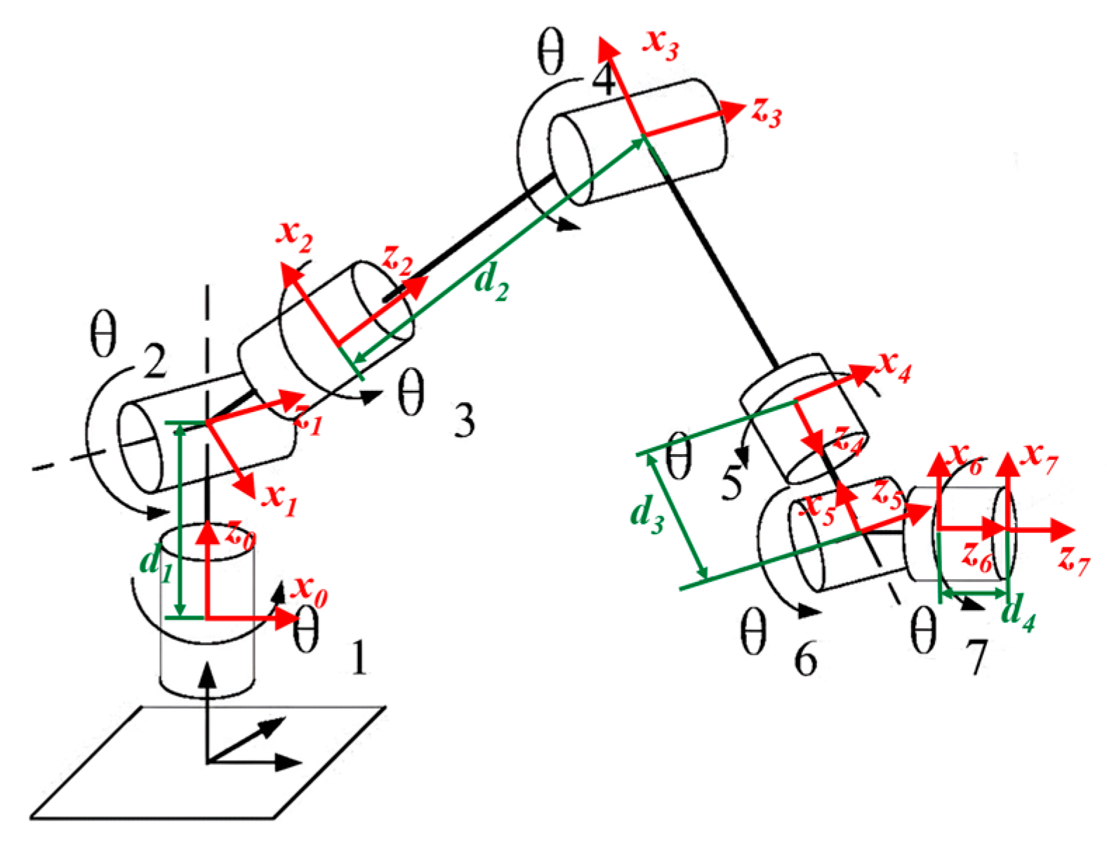
This chapter takes the seven-degree-of-freedom redundant manipulator as the research object. It has seven degrees of freedom, and each degree of freedom is a rotation joint, as shown in Figure 1. It adopts the SRS configuration (also called the “3-1-3” configuration), which consists of three shoulder joints, one elbow joint, and three wrist joints.
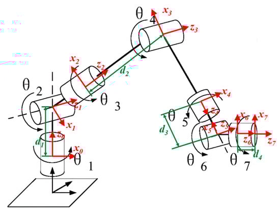
Figure 1.
SRS-configured manipulator.
In order to express the relationship between the various links of the redundant manipulator, the standard D-H method is used for modeling. The D-H parameters are shown in Table 1:

Table 1.
Redundant robot D-H parameter table.
According to the standard D-H modeling method, (1) the coordinate system is rotated degrees around the axis so that and are parallel to each other; (2) the coordinate system is translated along the axis by so that and are collinear; (3) the coordinate system is translated along the axis by so that the origins of and coincide; and (4) the coordinate system is rotated degrees around the axis to align and . Therefore, the homogeneous transformation matrix between the two links of the robot arm can be described as
For the two adjacent coordinate systems and , represents a rotation of around the axis. represents the translation distance along the axis. The meanings of and are the same as above. Therefore, the homogeneous transformation matrix of two adjacent joints of the robot could be described as
According to the right multiplication rule, the joint transformation matrices (i = 1, 2, …, n) are multiplied sequentially to obtain the robot transformation matrix:
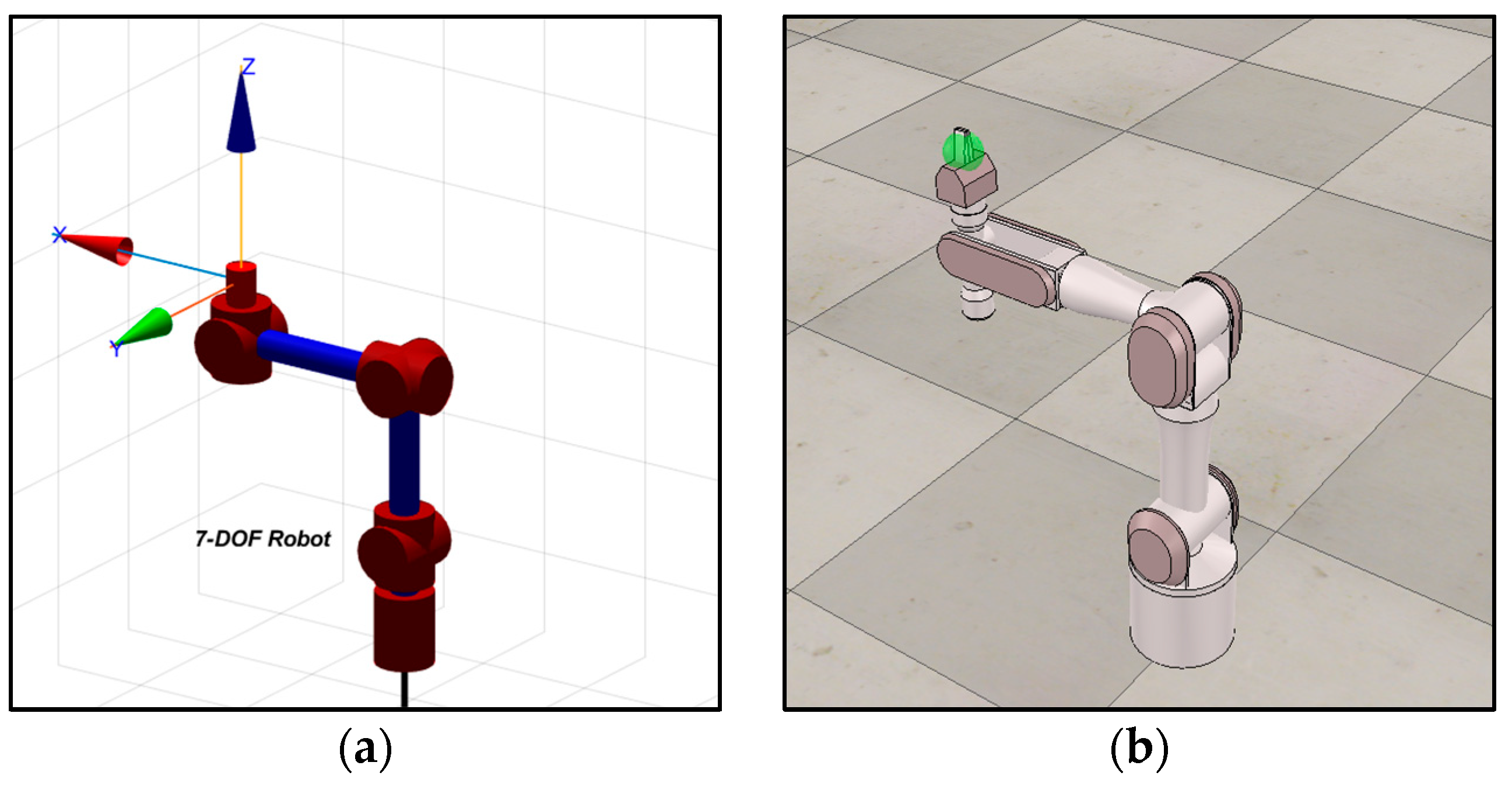
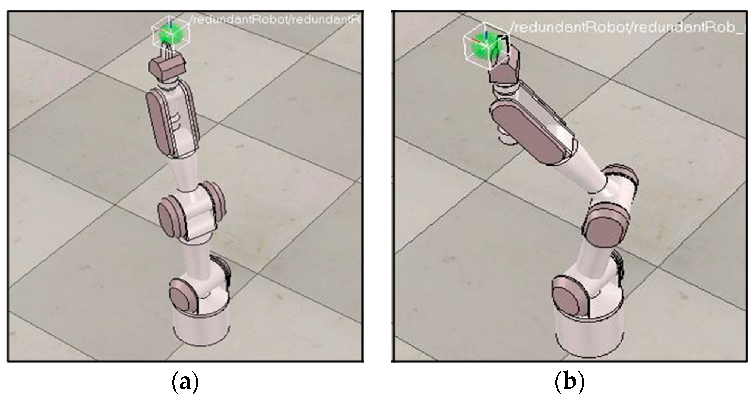
A robot model generated using MATLAB Robot Toolbox (9.10) and CoppeliaSim Edu 4.10 (V-Rep) is shown in Figure 2.

Figure 2.
Manipulator model. (a) Manipulator in MATLAB environment. (b) Manipulator in CoppeliaSim environment.
2.2. Inverse Kinematics Analysis
Firstly, eight sets of solutions for the redundant manipulator are calculated using the D-H parameter method. Inspired by the gradient projection method, an objective function is proposed, which simultaneously considers minimizing the end-effector error of the manipulator and the smoothness of joint motion, to obtain the optimal inverse solution of the robotic arm.
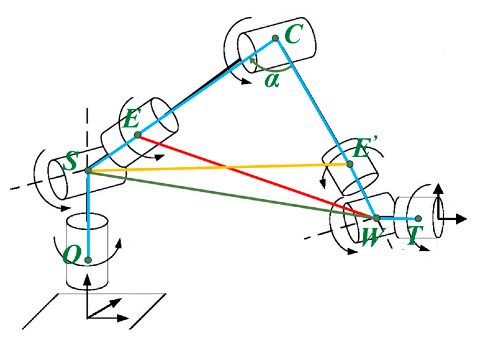
The redundant robot model established in Figure 1 is simplified, as shown in Figure 3. The coordinate changes and calculations in this paper are based on the coordinate system established in Figure 1. During the self-motion process, the attitude description of the manipulator depends on the joint angle . Given the coordinate transformation matrix of the end effector of the robotic arm in Cartesian space, the process of solving inverse kinematics is divided into the following three steps: First, the value of the elbow joint , which can be calculated based on the cosine theorem, is found. Secondly, by utilizing the known pose of the manipulator in Cartesian space, the reasonable range of can be calculated. Finally, a certain value is adopted within a reasonable range, and the angle values of the remaining joints of the manipulator can be calculated by taking the values of the end position and of the manipulator.
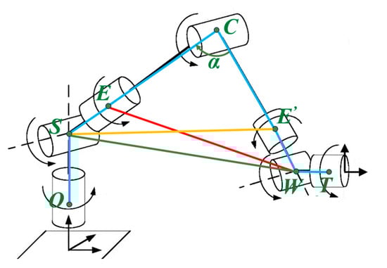
Figure 3.
Simplified model of seven-joint redundant robotic arm.
The process commences with solving for the origins of each link’s coordinate system, wherein the position of the robotic arm’s endpoint is predefined as point in the base coordinate framework. Consequently, the position of the wrist joint, denoted as point , is established within the coordinate system of the seventh joint as . The position matrix of point in the base coordinate system can be computed using Equation (4).
The origin coordinates of point S, representing the wrist joint, in the base coordinate system are thereby defined as . In triangle SEW, by applying the Cosine Law, we have
The position of point can be determined by Equation (6), and the unit vectors in a coordinate system with origin at point are given by Equation (7).
Point E undergoes rotation about the Z-axis of the coordinate system with its origin at point C, with a radial distance from the axis of rotation. The position of point E can be determined by the following equation (Equation (8)):
Up to this point, the determination of the origins for each coordinate system has been completed. Next, the seven joint angle values of the robotic arm will be solved separately.
(1) : From Figure 3, it can be seen that is the angle between the projection of on the plane and the axis .
Here, is a function that calculates the polar angle of a point (x, y) relative to the origin, which consists of the symbols of x and y, providing the correct range (−π, π] of angles. and represent the y and x of point E in the coordinate system, respectively.
(2) : is the angle between and .
(3) : To address this problem, it is essential to first compute the transformation matrix between the coordinate system and the base coordinate system. The angle of is the angle between the projection of onto a given plane and the -axis within the coordinate system associated with the second joint.
Here, and represent the coordinates of point E in the and coordinate systems, respectively.
(4) : is the angle between and .
(5) : is the angle between the projection of on the plane and the -axis.
(6) : is the angle between and .
(7) : The rotation matrix of the last joint is , calculated based on rotation.
According to the calculation characteristics of the inverse trigonometric function, , , and each have two different solutions. Given the pose coordinates of a set of end effectors of a robotic arm, eight sets of solutions corresponding to seven joint angles can be obtained. The set consisting of these eight solutions is defined as A.
Eight sets of solutions for a redundant manipulator can be obtained using the DH parameter method. Inspired by the gradient projection method, this paper proposes a method for obtaining the optimal solution, specifically by designing an objective function. This approach considers both the positional and orientational differences at the end effector of the manipulator, as well as the smoothness and energy efficiency of the robotic arm’s joint movements. The optimal solution for the robotic arm is obtained by minimizing the objective function . The design of is outlined as follows:
The calculation process of , which measures the attitude error by calculating the Frobenius norm error of the rotation matrix, is as follows:
Here, and are the end positions and postures calculated based on the joint angle . and are the expected positions and postures, and and are weight factors. Specifically, is the weight of smoothness, and n is the number of joints.
The process of finding the optimal solution for can be expressed as follows:
Here, is a set of joint vectors derived from the vector set obtained by using the arm angle parameter method mentioned above.
2.3. Simulation and Verification
This section outlines a validation experiment for the optimal inverse kinematics solution described in the previous section, using the Robotic Toolbox in MATLAB (9.10) and the robot simulation software CoppeliaSim (Edu 4.1.0) Perform to carry out inverse kinematics modeling and simulation of a seven-degree-of-freedom redundant robotic arm and to verify its accuracy. Figure 4 shows the robot in CoppeliaSim.
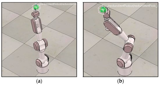
Figure 4.
The position of the manipulator in CoppeliaSim. (a) Initial pose. (b) Target pose.
As shown in Table 2, the theoretical angle obtained by the above calculation method was compared with the angle in the simulation environment by allowing the robotic arm to move smoothly from the initial pose to the final pose in the simulation environment.
Table 2.
Comparison of joint angles between starting and ending points of robots.
3. Motion Planning Algorithm for Manipulator
This chapter primarily focuses on the path planning of redundant manipulators in accessible spaces. It employs the rapidly exploring random tree (RRT) algorithm and the artificial potential field method for path planning, and compares their respective advantages and disadvantages.
3.1. Artificial Potential Field
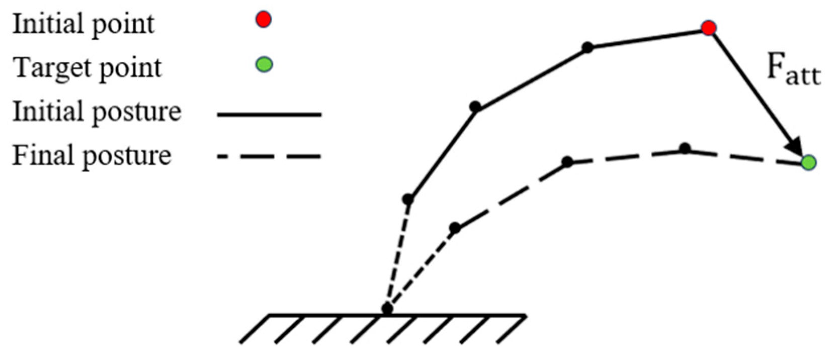
In basic artificial potential field methods, stability is typically only proven for point-to-point motion, with less emphasis placed on the stability of an end effector moving along a continuous trajectory. If there is a significant difference between the initial orientation and the target orientation, the motion path may become unachievable due to the need for higher speeds or larger torques.
In this section, this paper introduces an improved artificial potential field method that not only prioritizes the positioning of the end effector of the robotic arm, but also considers its attitude throughout the trajectory planning and obstacle avoidance process.
Firstly, boundaries were introduced for the Cartesian space components to optimize the attraction field function, such that regardless of the difference between the initial pose and the target pose, the redundant robotic arm’s end effector can now reach the target pose at a consistent speed.
As illustrated in Figure 5, the fundamental principle of the artificial potential field method involves constructing a virtual gravitational potential field around the target location of the task. This field generates an attractive force that guides the manipulator toward the target. By constructing a virtual, repulsive potential field near obstacles, the robotic arm generates repulsive force. Therefore, the key to path planning based on the artificial potential field method can be described as solving for the appropriate potential field and the corresponding force .
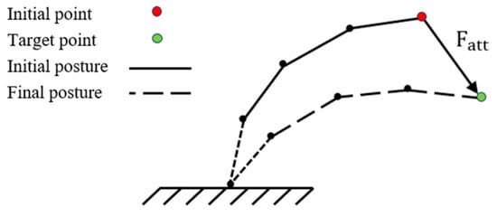
Figure 5.
Schematic diagram of artificial potential field method.
Generally, is defined as linearly converging to zero as the difference decreases, and infinitely increasing as increases:
where represents the position difference and represents the rotational attitude difference. However, defining only will lead to stability issues, as discontinuities may occur near the origin. To ensure the continuous variability in the potential field, a formula that accounts for the quadratic growth of can be used to define it as follows:
Here, denotes the attractive potential energy associated with the translation of the end effector, while represents the attractive potential energy related to the rotation of the end effector. is a weighting factor used to scale the influence of the attractive potential energy.
Obviously, excessive may lead to excessive and . To solve this problem, this paper uses a combination of quadratic potential and cone potential to define the attractive potential and the boundary .
The boundaries of the translation component (taking the dimension as an example) and the rotation component (taking the dimension as an example) are defined separately. The attraction of the target point to the robot is represented by the negative gradient of the gravitational potential field function, which directs the robot toward the target point.
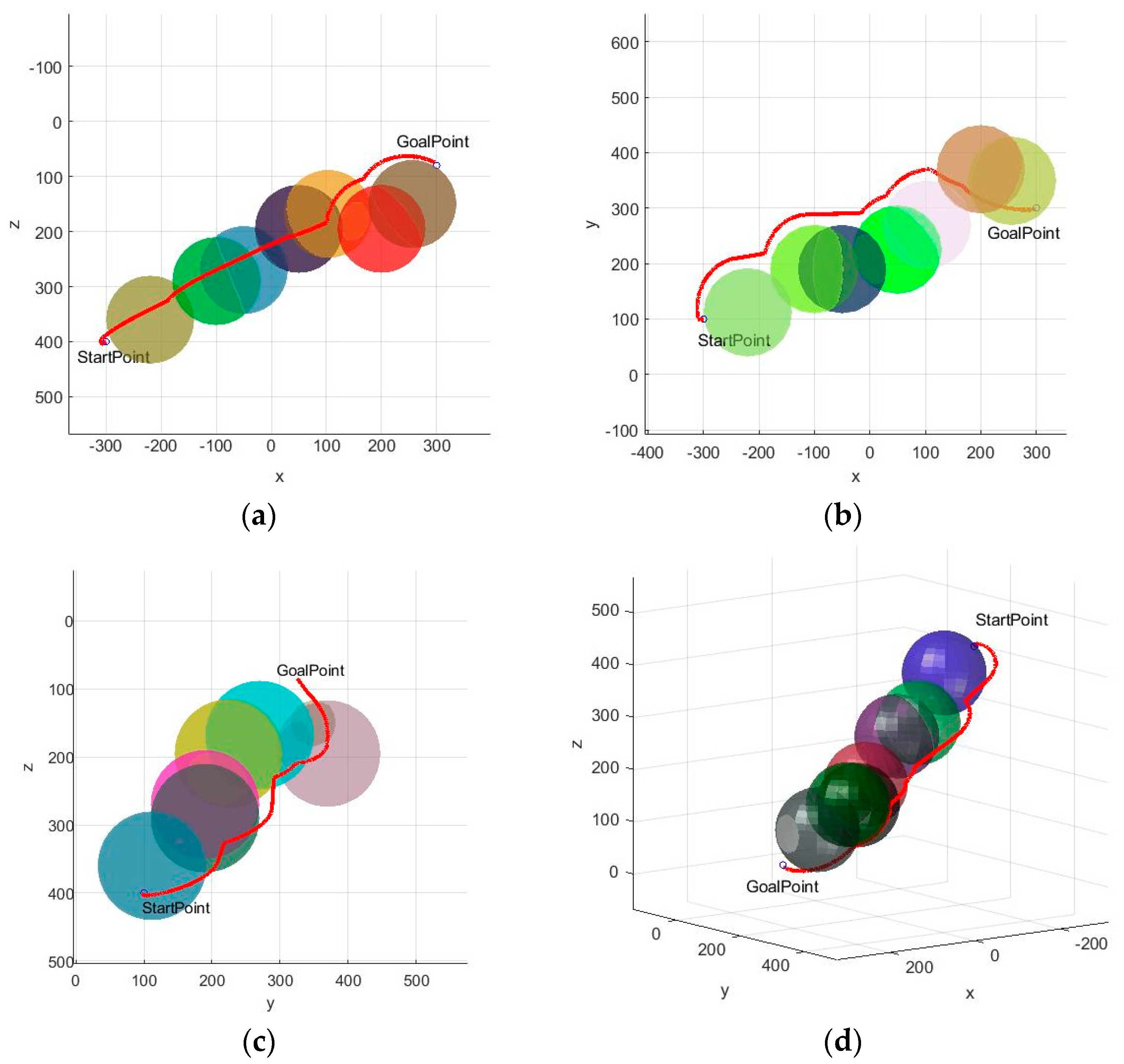
The simulation results are shown in Figure 6. The red curve represents the path, and there are randomly generated obstacles along the path.
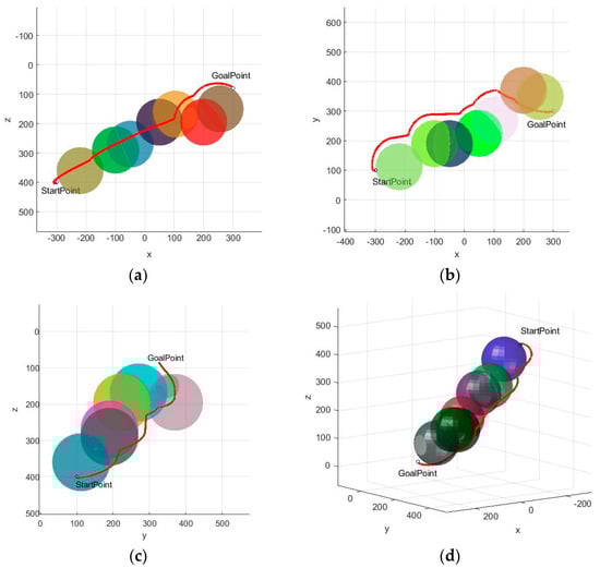
Figure 6.
Artificial potential field method for path planning in environment with obstacles. (a) XoZ surface projection. (b) XoY surface projection. (c) YoZ surface projection. (d) 3D perspective.
3.2. Rapidly Exploring Random Tree
The rapidly exploring random tree (RRT) algorithm typically starts with the initial point as the root node and generates a random search tree by randomly sampling and adding child nodes in the space. When the child nodes in the random search tree include the target point or enter the target area, a path made up of tree nodes from the initial node to the target node can be identified within the tree. The pseudocode of the RRT algorithm is illustrated in Algorithm 1.
| Algorithm 1 Rapidly Exploring Random Tree Algorithm Pseudo Code | |
| Input: | qS, qG, λ |
| Output: | T |
| 1: | T init = qS |
| 2: | for k = 1 : K do |
| 3: | qrand ← GetRandomNode() |
| 4: | q_closest ← NearNeighbor(T, qrand) |
| 5: | qnew ← SteerNode (qrand, qclosed, λ) |
| 6: | if CollosionFree() then |
| 7: | T.add_vertex(qnew) |
| 8: | end if |
| 9: | if GettheGoal then |
| 10: | return T |
| 11: | end if |
| 12: | end for |
In the above algorithm, qS represents the starting point, qG represents the ending point, λ represents the growth step size, and T represents the established random tree. The key explanations of the functions in the algorithm are as follows:
(1) NearNeighbor ()—Find Nearest Node: This function retrieves the nearest node Q in the random tree T given a randomly selected node G. The nearest node is determined according to a specific formula.
(2) SteerNode ()—Extension: This function involves creating a new node by extending a step size (represented by λ) from one configuration space node q1 toward another node q2. The representation of this function is as follows:
(3) CollisionFree ()—Collision Detection: This function is responsible for performing collision detection on the paths generated between nodes in two configuration spaces. Its purpose is to determine whether these paths are free of obstacles and thus safe for traversal.
(4) GetheGoal ()—Arrival Judgment: This function is used to determine whether the new node of the random tree is sufficiently close to the target node. If the new node is close, the function returns true; otherwise, the loop operation continues. The judgment formula is as follows:
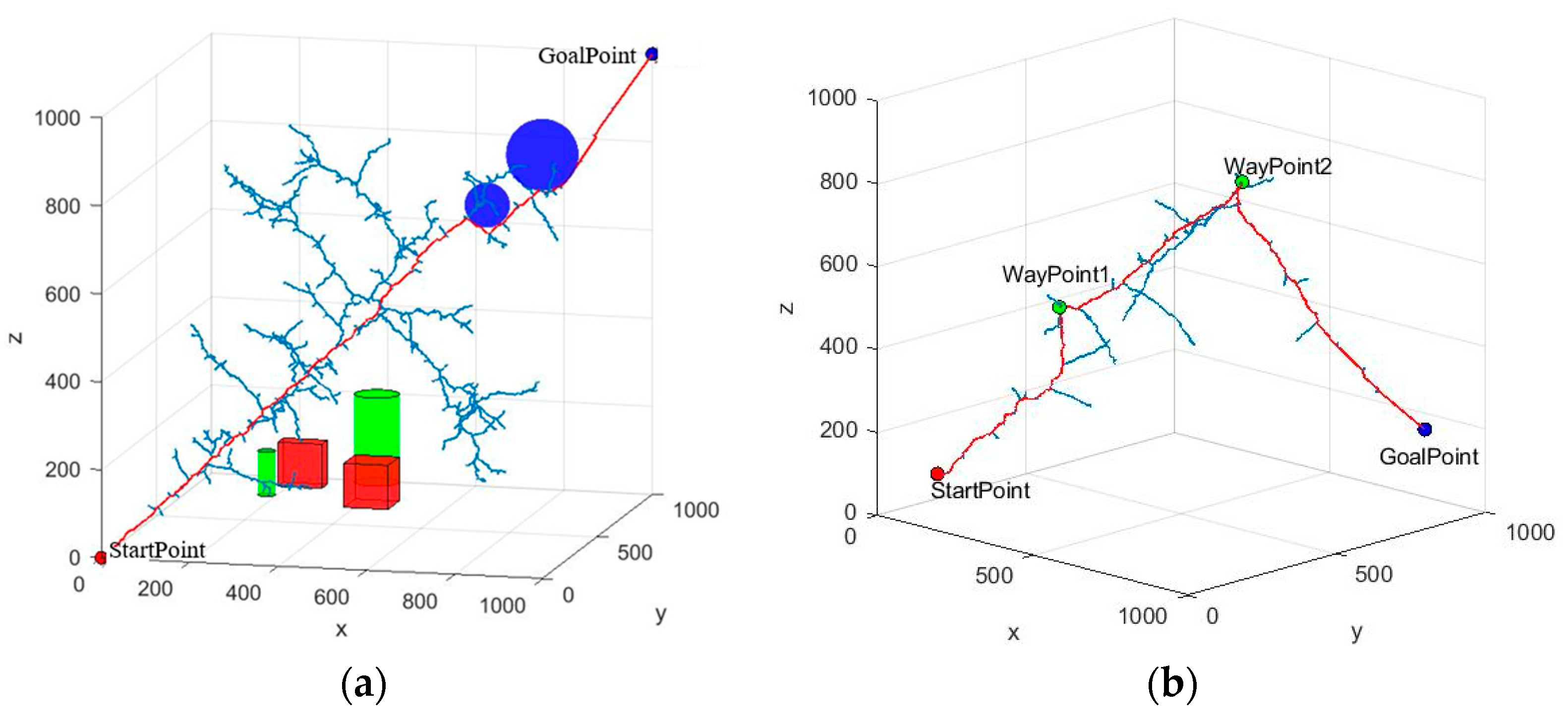
The simulation in MATLAB is shown in Figure 7. Figure 7a represents the path planning based on the RRT algorithm in an obstacle-free environment. The blue line represents the random number generated by the RRT algorithm during path generation, while the red line represents the final effective path generated. Figure 7b represents the path planning that requires the path to pass through a specific intermediate point in an obstacle-free environment. In RRT-based path planning, WayPoints can be specified. The red and blue points are the StartPoint and GoalPoint points, respectively, and the green point is the designated WayPoint. It can be seen that in an obstacle-free environment, the RRT algorithm does not generate many random numbers, making it easy to find a feasible path.
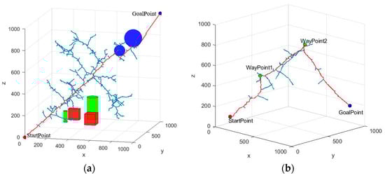
Figure 7.
RRT algorithm path planning. (a) Environment with obstacles. (b) Specifying WayPoints.
4. Conclusions
In conclusion, this paper successfully presented a comprehensive approach addressing the challenge of computing the optimal solution for inverse kinematics in redundant robots. By employing the D-H parameter method, we effectively derived eight distinct sets of vector solutions, significantly enhancing the solution space for these complex systems. The novelty lies in the tailored objective function, meticulously designed to gauge both the precision of the inverse kinematics solutions and the fluidity of joint motions. This function’s adaptability, achieved through adjustable weighting factors, empowers users to select solutions that cater to varying operational needs, thereby underlining the practical utility of our proposed method.
Furthermore, our work innovates path planning by introducing an enhanced artificial potential field algorithm. This improvement effectively tackles issues pertaining to discontinuities in gravitational potential during planning and mitigates excessive joint torques, which are common pitfalls in conventional methods.
Validation through simulations in the coupled environments of MATLAB’s Robot Toolbox and CoppeliaSim underscored the effectiveness and robustness of our methodologies. The joint angles obtained using the inverse solution method proposed in this article have an error of no more than 0.01 rad compared to the angles obtained in the CoppeliaSim simulation environment. Although the optimization objective function is added to the calculation process, there is no significant increase in computational complexity and duration, and the computation time remains basically unchanged. Future work may explore real-world implementations and further optimizations, but this study undeniably charts a promising course for enhancing the precision, adaptability, and efficiency of redundant robot operations.
Author Contributions
Conceptualization, L.C.; Methodology, X.Z. and L.C.; Software, X.Z.; Validation, X.Z. and L.C.; Resources, W.D.; Writing—original draft, X.Z. and L.C.; Writing—review & editing, X.Z.; Supervision, C.L. All authors have read and agreed to the published version of the manuscript.
Funding
This research received no external funding.
Data Availability Statement
The data presented in this study are available on request from the corresponding author.
Conflicts of Interest
The authors declare no conflict of interest.
References
- Zhang, Y.; Jia, Y. Motion planning of redundant dual-arm robots with multicriterion optimization. IEEE Syst. J. 2023, 17, 4189–4199. [Google Scholar]
- Suzuki, H.; Yukawa, H.; Minamizawa, K.; Tanaka, Y. Redundant Multi-DoF Robot Arm Co-operation through the Body Integration System. In Proceedings of the 2023 32nd IEEE International Conference on Robot and Human Interactive Communication (RO-MAN), Busan, Republic of Korea, 28–31 August 2023; IEEE: Piscataway, NJ, USA, 2023; pp. 2671–2676. [Google Scholar]
- Lu, Z.; Wang, N.; Shi, D. DMPs-based skill learning for redundant dual-arm robotic synchronized cooperative manipulation. Complex Intell. Syst. 2022, 8, 2873–2882. [Google Scholar]
- Peng, Y.; Nabae, H.; Funabora, Y.; Suzumori, K. Controlling a peristaltic robot inspired by inchworms. Biomim. Intell. Robot. 2024, 4, 100146. [Google Scholar]
- Zhang, C.; Chen, J.; Li, J.; Peng, Y.; Mao, Z. Large language models for human-robot interaction: A review. Biomim. Intell. Robot. 2023, 3, 100131. [Google Scholar]
- Raza, S.J.A.; Dastider, A.; Lin, M. Survivable hyper-redundant robotic arm with bayesian policy morphing. In Proceedings of the 2020 IEEE 16th International Conference on Automation Science and Engineering (CASE), Hong Kong, China, 20–21 August 2020; IEEE: Piscataway, NJ, USA, 2020; pp. 1–7. [Google Scholar]
- Sulaiman, S.; Sudheer, A.P. Dexterity analysis and intelligent trajectory planning of redundant dual arms for an upper body humanoid robot. Ind. Robot. Int. J. Robot. Res. Appl. 2021, 48, 915–928. [Google Scholar]
- Qiu, Z.; Zhao, J.; Wu, C.; Wang, W.; Wang, M.; Bao, G. Design and Experiment of Super Redundant Continuous Arm Driven by Pneumatic Muscle. In Proceedings of the Intelligent Robotics and Applications: 14th International Conference, ICIRA 2021, Yantai, China, 22–25 October 2021; Proceedings, Part I 14. Springer International Publishing: Berlin/Heidelberg, Germany, 2021; pp. 219–231. [Google Scholar]
- Kim, S.; Yun, S.; Shin, D. Numerical quantification of controllability in the null space for redundant manipulators. Appl. Sci. 2021, 11, 6190. [Google Scholar] [CrossRef]
- Khaleel, H.Z. Enhanced solution of inverse kinematics for redundant robot manipulator using PSO. Eng. Technol. J. 2019, 37. [Google Scholar]
- Mu, Z.; Yuan, H.; Xu, W.; Liu, T.; Liang, B. A segmented geometry method for kinematics and configuration planning of spatial hyper-redundant manipulators. IEEE Trans. Syst. Man Cybern. Syst. 2018, 50, 1746–1756. [Google Scholar]
- Zhou, S.; Liu, H.; Jiang, C.; Du, H.; Gan, Y.; Chu, Z. Research on kinematics solution of 7-axis redundant robot based on self-motion. In Proceedings of the 2020 Chinese Automation Congress (CAC), Shanghai, China, 6–8 November 2020; IEEE: Piscataway, NJ, USA, 2020; pp. 2622–2627. [Google Scholar]
- Shi, J.; Mao, Y.; Li, P.; Liu, G.; Liu, P.; Yang, X.; Wang, D. Hybrid mutation fruit fly optimization algorithm for solving the inverse kinematics of a redundant robot manipulator. Math. Probl. Eng. 2020, 2020, 6315675. [Google Scholar]
- Park, S.O.; Lee, M.C.; Kim, J. Trajectory planning with collision avoidance for redundant robots using jacobian and artificial potential field-based real-time inverse kinematics. Int. J. Control Autom. Syst. 2020, 18, 2095–2107. [Google Scholar]
- Chen, Z.M.; Guo, Y.; Xu, Z.G.; Ji, C.Y.; Yanwen, L. Inverse Kinematic Algorithm for 8-DOF Redundant Manipulators Based on Weighted Least-Norm Method and Parameterization Method. Res. Sq. 2021; preprint. [Google Scholar]
- Cheng, M.; Han, Z.; Ding, R.; Zhang, J.; Xu, B. Development of a redundant anthropomorphic hydraulically actuated manipulator with a roll-pitch-yaw spherical wrist. Front. Mech. Eng. 2021, 16, 698–710. [Google Scholar]
- Ricardo Xavier da Silva, S.; Schnitman, L.; Cesca Filho, V. A Solution of the Inverse Kinematics Problem for a 7-Degrees-of-Freedom Serial Redundant Manipulator Using Gröbner Bases Theory. Math. Probl. Eng. 2021, 2021, 6680687. [Google Scholar]
- Haug, E.J.; Peidro, A. Redundant manipulator kinematics and dynamics on differentiable manifolds. J. Comput. Nonlinear Dyn. 2022, 17, 111008. [Google Scholar]
- Vu, M.N.; Beck, F.; Schwegel, M.; Hartl-Nesic, C.; Nguyen, A.; Kugi, A. Machine learning-based framework for optimally solving the analytical inverse kinematics for redundant manipulators. Mechatronics 2023, 91, 102970. [Google Scholar]
- Dereli, S.; Köker, R. Calculation of the inverse kinematics solution of the 7-DOF redundant robot manipulator by the firefly algorithm and statistical analysis of the results in terms of speed and accuracy. Inverse Probl. Sci. Eng. 2020, 28, 601–613. [Google Scholar]
- Perrusquía, A.; Yu, W.; Li, X. Multi-agent reinforcement learning for redundant robot control in task-space. Int. J. Mach. Learn. Cybern. 2021, 12, 231–241. [Google Scholar]
- Tringali, A.; Cocuzza, S. Globally optimal inverse kinematics method for a redundant robot manipulator with linear and nonlinear constraints. Robotics 2020, 9, 61. [Google Scholar] [CrossRef]
- Safeea, M.; Bearee, R.; Neto, P. A modified DLS scheme with controlled cyclic solution for inverse kinematics in redundant robots. IEEE Trans. Ind. Inform. 2021, 17, 8014–8023. [Google Scholar]
- Ferrentino, E.; Chiacchio, P. On the optimal resolution of inverse kinematics for redundant manipulators using a topological analysis. J. Mech. Robot. 2020, 12, 031002. [Google Scholar]
- Tang, J.; Pan, R.; Zhou, S.; Wang, W.; Zou, R. An improved artificial potential field method integrating simulated electric potential field. Electron. Opt. Control 2020, 27, 69–73. [Google Scholar]
- He, N.; Su, Y.; Fan, X.; Liu, Z.; Wang, B. Dynamic path planning of mobile robot based on artificial potential field. In Proceedings of the 2020 International Conference on Intelligent Computing and Human-Computer Interaction (ICHCI), Sanya, China, 4–6 December 2020; IEEE: Piscataway, NJ, USA, 2020; pp. 259–264. [Google Scholar]
- Bing-Wei, Z.; Feng, J.; Yan, C.; Yu, S.; Yi-Hong, L. Path planning of artificial potential field method based on simulated annealing algorithm. Comput. Eng. Sci. Jisuanji Gongcheng Yu Kexue 2022, 44, 746. [Google Scholar]
- Tian, Y.; Zhu, X.; Meng, D.; Wang, X.; Liang, B. An overall configuration planning method of continuum hyper-redundant manipulators based on improved artificial potential field method. IEEE Robot. Autom. Lett. 2021, 6, 4867–4874. [Google Scholar]
- Sepehri, A.; Moghaddam, A.M. A motion planning algorithm for redundant manipulators using rapidly exploring randomized trees and artificial potential fields. IEEE Access 2021, 9, 26059–26070. [Google Scholar]
Disclaimer/Publisher’s Note: The statements, opinions and data contained in all publications are solely those of the individual author(s) and contributor(s) and not of MDPI and/or the editor(s). MDPI and/or the editor(s) disclaim responsibility for any injury to people or property resulting from any ideas, methods, instructions or products referred to in the content. |
© 2024 by the authors. Licensee MDPI, Basel, Switzerland. This article is an open access article distributed under the terms and conditions of the Creative Commons Attribution (CC BY) license (https://creativecommons.org/licenses/by/4.0/).