Transient Synchronous Stability Modeling and Comparative Analysis of Grid-Following and Grid-Forming New Energy Power Sources

Abstract

New energy power sources can be categorized into grid-following and grid-forming types based on their synchronization characteristics with the grid. Due to the different basic control operation principles of these two types of new energy power sources, they can lead to the instability of the grid-connected system through different paths. A mathematical model is established to describe the dynamic characteristics of the grid-following and the grid-forming new energy power resources, and the control block diagram of the nonlinear dynamic characteristic equation is compared and analyzed. The similarity between grid-following and grid-forming new energy power supply is revealed, and we preliminarily discuss the influencing factors of the stability of new energy sources. Using a single-machine infinite system model, the influence of key control parameters on transient stability is separately investigated for grid-following and grid-forming types. The influence of the converter synchronous loop control parameters on the system is verified, and the factors affecting the stability are discussed in combination with current limiting and frequency limiting. The research will provide reference for the design of a new energy power grid connection system.

1. Introduction

As the construction and development of new energy power systems continue, new energy sources, such as wind and solar energy, will become one of the main power sources in China’s power grid. By the end of 2022, the total installed capacity of wind and solar energy in China exceeded 700 million kilowatts, and the planned total installed capacity is expected to reach 1.2 billion kilowatts by 2030, accounting for 56.1% [1]. This trend indicates a significant increase in the scale of grid integration.

New energy sources integrate into the grid mainly through power electronic converters [2]. Unlike traditional synchronous power sources, these converters have distinct physical structures and control strategies, characterized by low inertia and under-damping. These traits pose new challenges to the safe and stable operation of the traditional power grid [3]. The stability of new energy power sources in grid-connected systems has become a major issue that hinders the further increase in the proportion of new energy and power electronic devices [4]. Therefore, exploring the factors influencing the stability of new energy sources is crucial.

The two main types of grid-connected inverters for new energy power sources are grid-following (GFL) and grid-forming (GFM) types. In this article, we define the grid-following-type and grid-forming-type inverters as grid-following new energy power sources and grid-forming new energy power sources, respectively.

Grid-following new energy power sources are essentially voltage-oriented current sources that track the phase of the existing grid voltage using a phase-locked loop [5]. This allows them to operate in synchronization with the grid. Grid-following converters have relatively simple control implementation and are widely used in wind and photovoltaic grid-connected systems. On the other hand, grid-forming inverters are essentially voltage-oriented power sources that synchronize with synchronous machines [6,7]. They adjust the output voltage frequency by exchanging power with the grid. Grid-forming inverters can maintain synchronization with the grid without needing a phase-locked loop and have the capability to autonomously generate voltage and frequency.

Grid-forming converters and grid-following converters exhibit distinct characteristics across various aspects. In [8], models for GFM and GFL converters were constructed, indicating that a higher penetration of GFM converters can enhance the system’s voltage and frequency stability compared to GFL converters. Additionally, the authors of [9] employed the D-partition method and noted that GFM converters demonstrated superior stability in weak grid conditions, whereas GFL converters showed greater stability in strong grid conditions. The authors of [10] conducted a comparative study on the frequency support capabilities of GFM and GFL converters, revealing that GFM converters consistently provided better frequency support than GFL converters. Therefore, the grid-connection characteristics of grid-following converters and grid-forming converters need to be studied separately.

Regarding the synchronization characteristics of the converters, the authors of [11] pointed out that considering grid impedance, frequency droop control in stand-alone inverters and phase-locked loops in grid-following inverters share certain structural similarities. Some scholars have unified the synchronization principles of grid-connected and stand-alone asynchronous power sources using the concept of duality [12]. The authors of [13] pointed out that there are certain similarities in the dynamic characteristics between inverters and synchronous machines. Furthermore, research has been conducted analyzing the small-signal stability of a single-inverter infinite bus system by describing its dynamic characteristics using the inertia coefficient, damping coefficient, and synchronizing coefficient [14]. In some respects, there are certain similarities or correspondences between grid-following and grid-forming new energy power sources. However, there is limited literature discussing the comparative analysis of their characteristics and the establishment of a unified model for these two types of asynchronous generators. Therefore, it is necessary to model and analyze these two types of new energy power sources and discuss their characteristics.

The authors of [15] indicated that traditional “synchronism stability” is no longer suitable for new power systems integrating asynchronous electromechanical sources. Therefore, the concept of “generalized synchronism stability” was proposed. Currently, numerous studies have analyzed the synchronism stability issues of grid-connected inverters, which could mainly be divided into small-disturbance and large-disturbance scenarios.

Currently, most studies on the transient synchronism stability of inverters are focused on investigating small disturbances. These studies primarily involve constructing small-signal models of the synchronous units of renewable energy sources, such as state-space models and impedance models [16,17,18]. Linearization methods suitable for small-disturbance analysis are no longer effective for addressing such issues [19]. Compared to the small-disturbance stability, the large-disturbance synchronism stability exhibits a more complex nature. Current research indicates several primary analysis methods for this, including the phase plane method [20,21], Lyapunov function analysis [22], and methods analogous to traditional synchronous machine “power-angle curves” [23,24].

The grid-connected renewable energy system models have high-order and highly complex nonlinear terms [25,26]. Specific investigations into the nonlinear dynamics of inverters, multi-time-scale coupling, control mode switching, and related aspects are still in the process of deeper exploration [27]. Therefore, it is necessary to investigate the transient instability mechanism of asynchronous power sources under large disturbances. This study will present an innovative analysis from the viewpoint of large disturbances, identifying the critical factors that influence the transient synchronization stability of grid-forming converters (GFM) and grid-following converters (GFL). We conduct a comparative analysis of the transient synchronous stability characteristics of these two converter types, highlighting their inherent consistency. This research will offer technical support for the planning and design of future grids, especially for high penetration of renewable energy integration. The structure of the following sections is as follows: Section 2 will preliminarily establish second-order differential equations reflecting the dynamic characteristics of grid-following and grid-forming new energy power sources based on their control loops. Section 3 will obtain a unified form of the dynamic equations for new energy power sources and the corresponding control block diagram by comparing and analyzing the nonlinear dynamic characteristic equations of traditional synchronous generators and new energy power sources, and preliminarily identify the factors influencing the transient synchronous stability of new energy power sources. Section 4 will analyze the influence of the parameters of the internal control loop of new energy power sources on the stability of inverters under the condition of not considering frequency and current limiting. Section 5 will discuss the stability and influencing factors of new energy power systems considering the role of limiting elements through time-domain simulation comparisons. Finally, Section 6 will provide a summary of the entire article.

2. Modeling of New Energy Power Sources

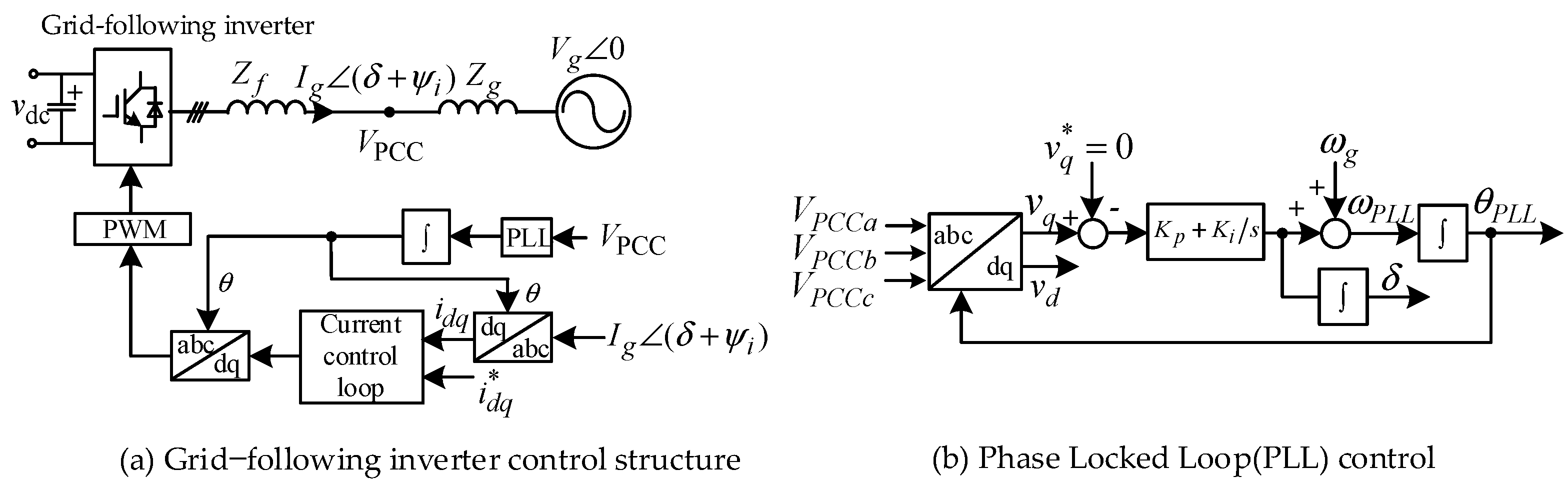
2.1. Grid-Following New Energy Power Sources

The grid-following inverter obtains the angle of the grid voltage at the point of connection through direct calculation or closed-loop control, which serves as the reference angle for the control of the inverter. The corresponding circuit and control structure are shown in Figure 1.

Figure 1a illustrates the control structure of grid-following new energy sources. Figure 1b depicts the control structure of the core synchronization unit of the sources (the phase-locked loop). It collects the phase angle of the voltage at the point of common coupling (V_PCCabc) and transforms it to the dq coordinate system through the Park transformation (Vdq). Vq is made to track its reference value, V_qref = 0, through proportional–integral (PI) control loops, and negative feedback loops control the output reference angle, θ_PLL. This angle, θ_PLL, is used to track the phase angle of the grid voltage. Here, ψ_i = arctan(i_q/i_d) represents the current reference angle, and $\delta ={\theta }_{\mathrm{P}\mathrm{L}\mathrm{L}}-{\theta }_g$ represents the difference between the output angle of the PLL and the grid voltage angle.

In the PI control loop, k_p and k_i are the proportional and integral gain of the PLL. For the infinite system shown in Figure 1, the PLL is used to achieve synchronization, and an L-type filter is implemented. According to the structure diagram of the grid-connected inverter shown in Figure 1a, the expression for the PCC point voltage can be written as follows:

$${\dot{v}}_{\mathrm{PCC}}={\dot{V}}_g+(R_g+j{X}_g)\dot{I}=V_g{e}^{j{\theta }_g}+(R_g+j{X}_g)\cdot (i_d^{*}+j{i}_q^{*})e^{j{\theta }_{PLL}}$$

(1)

where ${\dot{V}}_g$ is the grid voltage vector, while R_g and X_g are the line resistance and reactance values, respectively.

According to the control block diagram of the phase-locked loop (PLL) shown in Figure 1b, it can be inferred that the virtual power angle and speed of the PLL depend on the q-axis component of the PCC point voltage in the PLL coordinate system.

$$v_{PCCq}=\mathrm{Imag}({\dot{v}}_{PCC}{e}^{-j{\theta }_{PLL}})=X_g{i}_d^{*}+R_g{i}_q^{*}+{\displaystyle \frac{X_g{i}_d^{*}}{{\omega }_g}}({\omega }_{PLL}-{\omega }_g)-V_g\sin (\delta )$$

(2)

Therefore, when the grid short circuit is relatively low, the network equivalent reactance is large, and the PCC point voltage is greatly affected by the injected grid current of the inverter. The PCC point voltage, in turn, affects the injected current through the virtual power angle of the phase-locked loop, forming a closed-loop feedback loop.

The control bandwidth of the inner current loop of grid-connected inverters is usually several hundred hertz or even several kilohertz, while the bandwidth of the phase-locked loop is generally several tens of hertz. Therefore, during the operation of the phase-locked loop, it can be assumed that the control of the current loop has been completed, and the current can be considered as a constant value when considering the dynamics of the phase-locked loop.

$$\{\begin{array}{l}{I}_d=I_{dref}\\ I_q=I_{qref}\end{array}$$

(3)

Here, I_d is the output current d-axis component, I_dref is the reference value for the output current d-axis component, I_q is the output q-axis component, and I_qrf is the reference value for the output current q-axis component.

Based on the control block diagram of the phase-locked loop shown in Figure 2, we can obtain the second-order differential equation of the grid-connected inverter, as follows:

$$\left(1-k_p{I}_{dref}{L}_g\right)\ddot{\delta }=k_i\left(I_{dref}{L}_g\dot{\delta }-{\displaystyle \frac{k_p{V}_g\cos \delta }{k_i}}\dot{\delta }+I_{dref}{\omega }_n{L}_g+I_{qref}{R}_g-V_g\sin \delta \right)$$

(4)

where ω_n is the rated frequency of the grid.

For high-voltage-level transmission networks, in general, reactance is much larger than resistance, so ignoring the resistance, it can be obtained as:

$$\left(1-k_p{I}_{dref}{L}_g\right)\ddot{\delta }=k_i\left(I_{dref}{L}_g\dot{\delta }-{\displaystyle \frac{k_p{V}_g\cos \delta }{k_i}}\dot{\delta }+I_{dref}{\omega }_n{L}_g-V_g\sin \delta \right)$$

(5)

2.2. Grid-Forming New Energy Power Sources

Grid-forming inverters use the calculated power at the grid connection point as the input for outer loop power control, generating reference voltage and phase. The main outer loop synchronizing unit generates the grid-connection reference values. Active power control (APC) calculates the corresponding phase reference value based on the active power at the grid connection point. Reactive power control (RPC) generates the corresponding voltage amplitude reference value based on the reactive power at the grid connection point. The inner loop mainly uses voltage and current dual-loop control to control the output voltage and amplitude of the inverter. It is a power-oriented voltage source.

The core synchronization unit of grid-connected inverters is the APC. The classical control strategies for grid-connected inverters include power synchronization control, droop control, droop control with low-pass filtering, and virtual synchronization control. Among them, power synchronization control and droop control are equivalent to each other and are both first-order systems, which have simple and easy-to-design structures, but cannot achieve inertial support. Droop control with low-pass filtering and virtual synchronization control are equivalent to each other and can be classified as second-order systems. They can simulate the rotor motion characteristics and excitation characteristics of synchronous generators, enabling them to have equivalent inertial support and damping capabilities, and have stronger disturbance rejection performance. This paper mainly discusses droop control with filtering, and its corresponding circuit and control structure are shown in Figure 2.

Droop control is the simplest and most common grid-forming control strategy, which emulates the active-frequency (P-f) and reactive-voltage (Q-U) droop characteristics of synchronous generators. The expression for droop characteristics can be formulated as:

$$\{\begin{array}{l}\omega ={\omega }_0+m_p(P_{ref}-P)\\ V=V_0+m_q(Q_{ref}-Q)\end{array}$$

(6)

where m_p and m_q are the droop coefficients for active-power frequency and reactive-power voltage, respectively.

Droop control with low-pass filtering adds a low-pass filtering component (1/1 + sT_f) to the basic droop control, which filters out high-frequency harmonic signals while providing virtual inertial support. Therefore, the expression for droop characteristics with low-pass filtering can be formulated as:

$$\{\begin{array}{l}\omega ={\omega }_0+{\displaystyle \frac{m_p}{1+s{T}_{fp}}}\left(P_{ref}-P\right)\\ V=V_0+{\displaystyle \frac{m_q}{1+s{T}_{fq}}}\left(Q_{ref}-Q\right)\end{array}$$

(7)

where T_f is the time coefficients in the low-pass filter.

In Figure 2, G_FD = m/(1 + sTf), where m is the droop control gain and Tf is the time constant of the first-order filter used for power calculation. The external circuit adopts an LCL-type filter. In voltage–current dual-loop control, the bandwidth of the voltage–current loop is generally 2–3 orders of magnitude higher than that of the synchronization loop, which means that the response speed of the voltage–current inner loop is much faster, so the voltage can be considered constant.

The active power, P, generated at the grid-connected point of the inverter can be represented as:

$$P={\displaystyle \frac{1}{Z_g}}\cdot (V_{PCC}^2\cos {\theta }_{zg}-V_{PCC}{V}_g\cos (\delta +{\theta }_{zg}))$$

(8)

According to the active-frequency droop control block diagram, the second-order differential equation for the grid-forming inverter can be obtained as:

$$T_f\ddot{\delta }=-\dot{\delta }+m\left(P_{ref}-{\displaystyle \frac{1}{Z_g}}\cdot (V_{PCC}^2\cos {\theta }_{zg}-V_{PCC}{V}_g\cos (\delta +{\theta }_{zg}))\right)$$

(9)

where V_PCC is the magnitude of the grid-connected point voltage, Z_g is the magnitude of the line impedance, θ_zg is the angle of the line impedance, and δ is the phase difference between the grid-connected point voltage and the grid phase angle.

If we ignore the line resistance and assume the line to be purely inductive, Equation (7) can be simplified as:

$$T_f\ddot{\delta }=-\dot{\delta }+m\left(P_{ref}-{\displaystyle \frac{V_{\mathrm{PCC}}{V}_g\sin \delta }{X_g}}\right)$$

(10)

where X_g is the value of the line inductance.

3. Model Comparison of Synchronous Generator and New Energy Power Source

The rotational equation of a conventional synchronous generator in state-space representation can be described as:

$$\{\begin{array}{l}{\displaystyle \frac{d{\delta }^{\prime }}{dt}}={\omega }^{\prime }-{\omega }_0^{\prime }\\ H{\displaystyle \frac{d{\omega }^{\prime }}{dt}}=P_m-P_E-D({\omega }^{\prime }-{\omega }_0^{\prime })\end{array}$$

(11)

where the symbol ${\delta }^{\prime }$ is the power angle of the synchronous machine, H is the inertia time constant of the synchronous machine, D is the damping coefficient of the synchronous machine, P_m represents the mechanical active power, and P_E is the electromagnetic power.

Traditional synchronous generators, during normal operation, transfer a portion of the rotor’s kinetic energy in the form of electrical energy, while the remaining portion of the kinetic energy is reflected in the form of rotational inertia due to the high-speed rotation of the rotor. When the system is disturbed, the rotor is able to continue storing and releasing energy, and the rotor inertia acts as a buffer, effectively suppressing frequency fluctuations. The damping coefficient primarily affects the rate of frequency change in the system. Increasing the damping coefficient can effectively reduce the amplitude of frequency oscillations and allow the system to quickly recover to a stable state in the event of a fault. Therefore, the magnitudes of the inertia time constant and damping coefficient both influence the dynamic characteristics and synchronous stability of the synchronous machine.

To compare the new energy power supply with the synchronous machine model, we can convert the nonlinear differential Equations (5), (10), and (11) into control block diagrams. It can be observed that the dynamic equation control block diagrams of the two types of new energy power supply and synchronous machine can be transformed into similar forms, as shown in Figure 3. Therefore, the dynamic characteristics equation of the new energy power supply can also be represented in a similar form as the synchronous machine, expressing an equivalent inertia time constant, damping coefficient, active power reference value, and actual active power output. We will discuss them separately.

Comparing (a) and (b) in Figure 3, we can obtain the equivalent active power reference value, P_1ref, equivalent actual output active power, P₁, equivalent inertia time constant, H₁, and equivalent damping coefficient, D₁, for the grid-type new energy power supply:

$$\{\begin{array}{l}{H}_1={\displaystyle \frac{1-K_P{I}_{dref}{L}_g}{K_I}}\\ D_1={\displaystyle \frac{K_P{V}_g\cos \delta }{K_I}}-I_{d\mathrm{ref}}{L}_g\\ P_1=V_g\sin \delta \\ P_{1ref}=I_{dref}{\omega }_0{L}_g\end{array}$$

(12)

As shown in the equation above, the equivalent inertia time constant and damping coefficient of the grid-type inverter are influenced by multiple parameters. The equivalent inertia time constant is negatively linearly related to the proportional gain, K_p, of the phase-locked loop, and inversely proportional to the integral gain, K_I. The equivalent damping coefficient, H₂, is directly proportional to K_p and inversely proportional to K_I. The maximum value of the equivalent actual output active power is directly proportional to the grid voltage, while the equivalent active power reference value is directly proportional to the line parameters. It is worth noting that for the equivalent actual output active power and equivalent active power reference value, their actual physical meaning is not a power value. From their expressions, it can be seen that their actual meaning should be voltage. However, changing this value has the same effect on the system stability. Here, the use of equivalent power is for the sake of expression uniformity.

Comparing (a) and (c) in Figure 3, we can obtain the equivalent active power reference value, P_2ref, equivalent actual output active power, P₂, equivalent inertia time constant, H₂, and equivalent damping coefficient, D₂, for the grid-forming new energy power supply:

$$\{\begin{array}{l}{H}_2={\displaystyle \frac{T_f}{m}}\\ D_2={\displaystyle \frac{1}{m}}\\ P_2={\displaystyle \frac{1}{X_g}}\cdot V_{PCC}{V}_g\sin \delta \\ P_{2ref}=P_{ref}\end{array}$$

(13)

The inertia coefficient, H₂, of the grid-forming inverter is directly proportional to the time constant, T_f, of the first-order filter used for power calculation, and inversely proportional to the power droop gain, m. The damping coefficient, D₂, is inversely proportional to the power droop gain, m. Therefore, without considering the voltage and current inner loop, the output active power, P₁, of the inverter is related to parameters such as the grid voltage and line parameters.

By comparing the control block diagrams transformed through dynamic equations, it is evident that the dynamic equations of grid-following and grid-forming new energy power sources can be transformed into forms similar to the synchronous machine rotor motion equations. Therefore, Equation (11) can be expressed in a unified form representing the dynamic equations of these three types of power sources. Combining Equations (12) and (13), we can determine the factors that influence the equivalent active power reference value, equivalent actual output active power, equivalent inertia coefficient, and equivalent damping coefficient of both grid-following and grid-forming new energy power supplies, as well as their positive or negative correlations. This information is summarized in Figure 4.

Figure 4 graphically shows the influence progress of the system parameters on the transient synchronous stability, i.e., the change in a parameter represented in the figure will lead to the change in the equivalent inertia coefficient (H), the damping coefficient (D), the reference value of the active power (P_ref), and the actual output active power (P) within the system, which, in turn, has a positive or negative influence on the transient synchronous stability of the system.

According to Figure 4, it can be observed that the factors affecting the stability of the grid-following new energy power supply are more complex compared to the factors affecting the stability of the grid-forming new energy power supply. The equivalent damping coefficient and inertia coefficient of the grid-following system are influenced by multiple factors, while the equivalent damping coefficient and inertia coefficient of the grid-forming system are only related to one or two influencing factors. It is worth noting that the equivalent damping coefficient of the grid-following system is related to δ, which means that the equivalent damping coefficient of the grid-following new energy power supply varies during the transient process. During operation, it is necessary to maintain a damping coefficient greater than 0, otherwise the system will face the risk of instability.

4. The Impact of Synchronization Loop Control Parameters on Stability

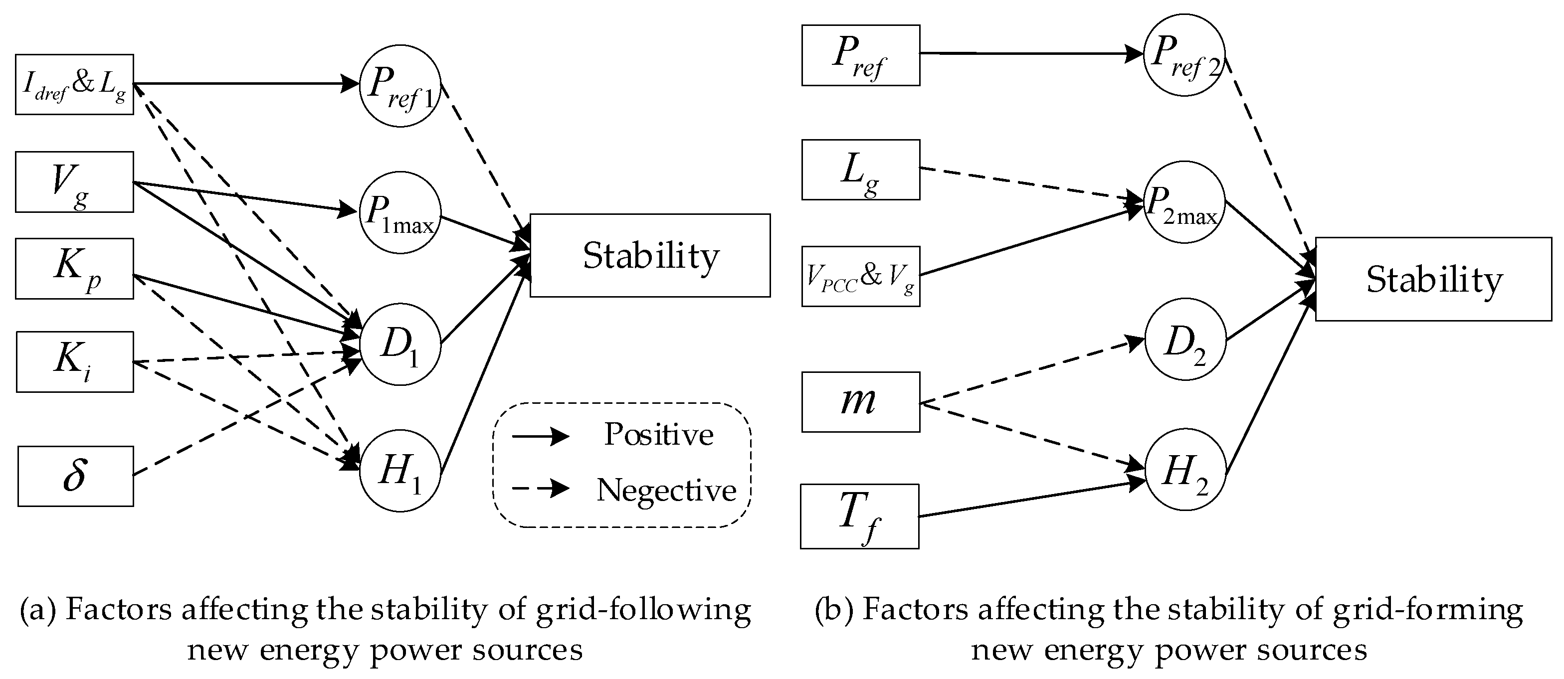
4.1. Key Factors Affecting the Stability of Grid-Following New Energy Power Supplies

The core synchronization unit of the grid-following new energy power supply is a phase-locked loop (PLL). The dynamic performance of the PLL is determined by the proportional gain (K_p) and integral gain (K_I). Therefore, setting the control parameters of the PLL is a crucial condition for system stability. Now, we consider a single grid-following new energy power supply infinite system, as shown in Figure 1, with specific parameters detailed in Appendix A,

Table A1. Single GFL infinite bus parameters.

System Parameters	Values	System Parameters	Values
Base frequency/Hz	50	Line inductance/pu	0.3
Base power/VA	1	Output active power/pu	1
Base voltage/V	1	Current loop proportional gain	0.25
Filter resistance/pu	0.001	Current loop integral gain	98.17
Filter reactance/pu	0.05	PLL proportional gain	62.83
Line resistance/pu	0.06	PLL integral gain	986.96

[28]. We will investigate the effects of the integral gain (K_I) and proportional gain (K_p) of the PLL on the stability of the grid-following inverter.

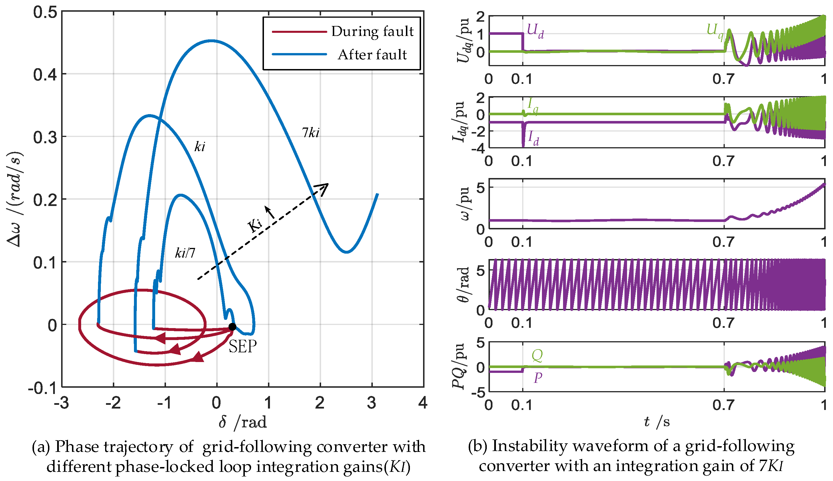
4.1.1. The Effect of Integral Gain (K_I) in PLL

In the presented single infinite system, a three-phase short-circuit fault occurred at the output of the inverter at 0.1 s, and the fault lasted for 0.6 s. The phase trajectory diagrams of the inverter during the fault process and after the fault was eliminated are plotted with phase-locked loop integral gains set as K_I/7, K_I, and 7K_I, as shown in Figure 5.

In Figure 5a, the vertical axis represents the frequency change, and the horizontal axis represents the relative change in the phase angle of the output voltage compared to the initial stable state. The red curve represents the phase trajectory diagram of the inverter’s state variables during the fault, and the blue curve represents the phase trajectory diagram after the fault was cleared. Starting from the initial point, if the phase trajectory diverges, the grid-following inverter is synchronized unstable. If the phase trajectory can converge to a stable equilibrium point in the phase plane, the inverter restores synchronous stability.

From Figure 5a, it can be seen that as the phase-locked loop integral gain increased from K_I/7 to KI and then to 7K_I, the movement trajectory of the inverter’s state variables gradually expanded. The longer the red region in the figure, the faster the response under the same fault duration, and the longer the trajectory deviating from the equilibrium point. This indicates that the inverter was gradually becoming unstable and had poorer anti-interference capability.

When the integral gain of the phase-locked loop reached 7K_I, the phase trajectory of the system could not return to the initial stable operating point after the fault was cleared, indicating that the system lost synchronization. Figure 5b shows the waveform of electrical quantities of the grid-following inverter’s phase-locked loop when the integral gain was unstable at 7K_I. Under the condition of a fault duration of 0.6 s, the inverter’s output voltage, current, active power, and reactive power all exhibited unstable oscillations, and the inverter’s angular frequency began to increase abnormally, leading to synchronization instability. From the simulation experiment, it can be concluded that an increase in the integral gain, K_I, will result in a faster dynamic response of the grid-following inverter, but it will also reduce the stability of the inverter under fault conditions.

Therefore, an increase in the integral gain will decrease the equivalent inertia coefficient, H₂, and the effective damping coefficient, D₂, of the grid-following inverter, resulting in reduced stability. This property is similar to synchronous generators.

4.1.2. The Effect of Proportional Gain (K_P) in PLL

With the same fault occurrence time and fault duration, the system simulation results are shown in Figure 6a when the proportional gain, K_p, was set to K_p/10, K_p, and 10K_p, respectively. As K_p increased, the equivalent damping coefficient, D₂, increased, indicating an increase in system stability. However, it also led to a decrease in the equivalent inertia time constant, H, representing a decrease in the inverter’s disturbance rejection capability. In Figure 6a, when the proportional gain was 10K_p, significant oscillations occurred at the equilibrium point after the fault was cleared. Therefore, the influence of K_p on the stability of the inverter is not a simple linear relationship. When the proportional gain was K_p/10, the phase trajectory diverged, and the phase-locked loop became unstable.

Figure 6b shows the waveform of various electrical quantities of the grid-following inverter when the proportional gain was K_p/10 and the system became unstable. At this time, the inverter’s output voltage, current, active power, and reactive power all exhibited non-periodic oscillations, and the angular frequency experienced abnormal increases. Although the frequency during the fault duration in Figure 6b remained near the rated value, it can be seen from Figure 6a that the phase difference continuously increased during the fault period. When the fault was cleared, the phase difference still approached −π, resulting in an irreversible increase in the output frequency of the phase-locked loop and causing system instability.

Based on the above, increasing the proportional gain, K_p, will lead to an increase in the system’s equivalent damping coefficient. Consequently, energy dissipation during the system’s dynamic processes will increase, making the system more prone to stability. However, as K_p increased, the equivalent inertia time constant, H, decreased, resulting in reduced disturbance rejection capabilities. When subjected to the same level of disturbance, the system will exhibit greater frequency oscillations internally.

4.2. Key Factors Affecting the Stability of Grid-Forming New Energy Power Supplies

A grid-forming inverter infinite system was constructed, as shown in Figure 2. The system parameters are detailed in Appendix A [28],

Table A2. Single GFM infinite bus parameters.

System Parameters	Values	System Parameters	Values
Base frequency/Hz	50	Power calculation Filter bandwidth/Hz	5
Base power/VA	1	Droop gain	0.05
Base voltage/V	1	Voltage loop integration gain	282.743
Source-side filter resistance/pu	0.01	Voltage loop proportional gain	0.012
Source-side filter reactance/pu	0.05	Current loop proportional gain	565.487
Filter capacitance/pu	0.02	Current loop integral gain	0.6
Grid-side filter reactance/pu	0.01	Output active power/pu	565.487
Grid-side filter resistance/pu	0.002	Line inductance/pu	0.1
Line resistance/pu	0.02

. At 0.1 s, a three-phase short-circuit fault occurred at the output of the inverter, with a fault duration of 0.02 s. The droop gains were set to m/10, m/3, and m, respectively, resulting in the phase trajectory shown in Figure 7a.

From Figure 7a, it can be observed that as the droop gain increased, the range of the system’s phase trajectory also increased. The inverter gradually tended toward an unstable state until the droop gain reached m, where the inverter’s output frequency experienced irreversible decline and the system lost synchronization. Figure 7b shows the waveform of electrical quantities for the grid-forming inverter when the droop gain was set to m, both during the occurrence of a three-phase short-circuit fault at the inverter’s output and after the fault was cleared. From the figure, it can be seen that when a three-phase short circuit occurred at the inverter’s port for 0.02 s, the inverter’s frequency significantly decreased and the output voltage and current exhibited irregular oscillations. At this point, the equipment lost synchronization with the grid. Therefore, increasing the droop gain (m) will lead to a decrease in the system’s damping coefficient and inertia coefficient, reducing the transient synchronizing stability of the system.

In summary, this section explored the effects of the proportional gain, K_P, integral gain, K_I, and droop gain, m, in the phase-locked loop of the grid-forming inverter on its stability. These parameters are factors that affect the stability of the inverter’s internal control loop. As analyzed earlier, this is because changes in the control parameters of the inverter’s internal loop altered the equivalent dynamic characteristic coefficients of the inverter, thereby affecting the system’s stability, either positively or negatively. An increase in the system’s equivalent damping coefficient increased system stability, making it more likely to stabilize after being disturbed. An increase in the system’s equivalent inertia slowed down the system’s response, but the delayed response time tended to stabilize the system and enhance its disturbance resistance.

5. Stability Factors of Renewable Energy Sources under the Limitation Effect

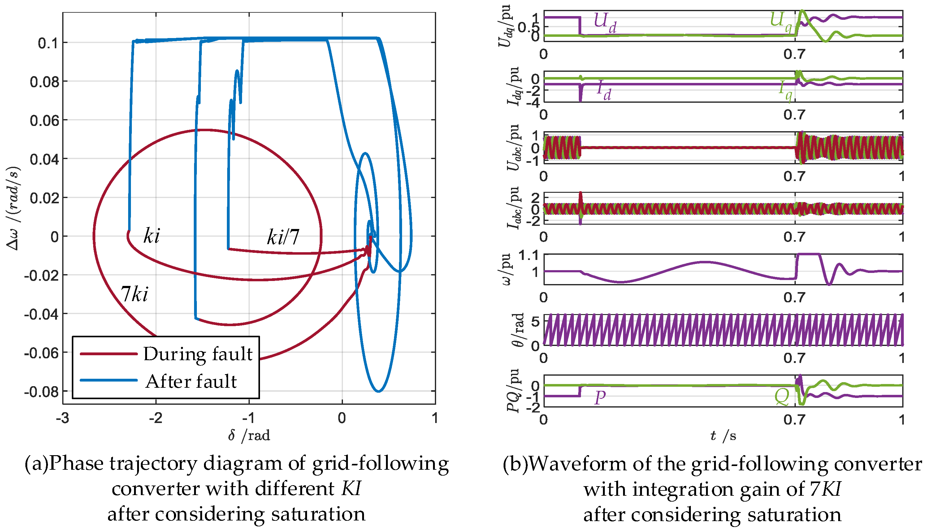
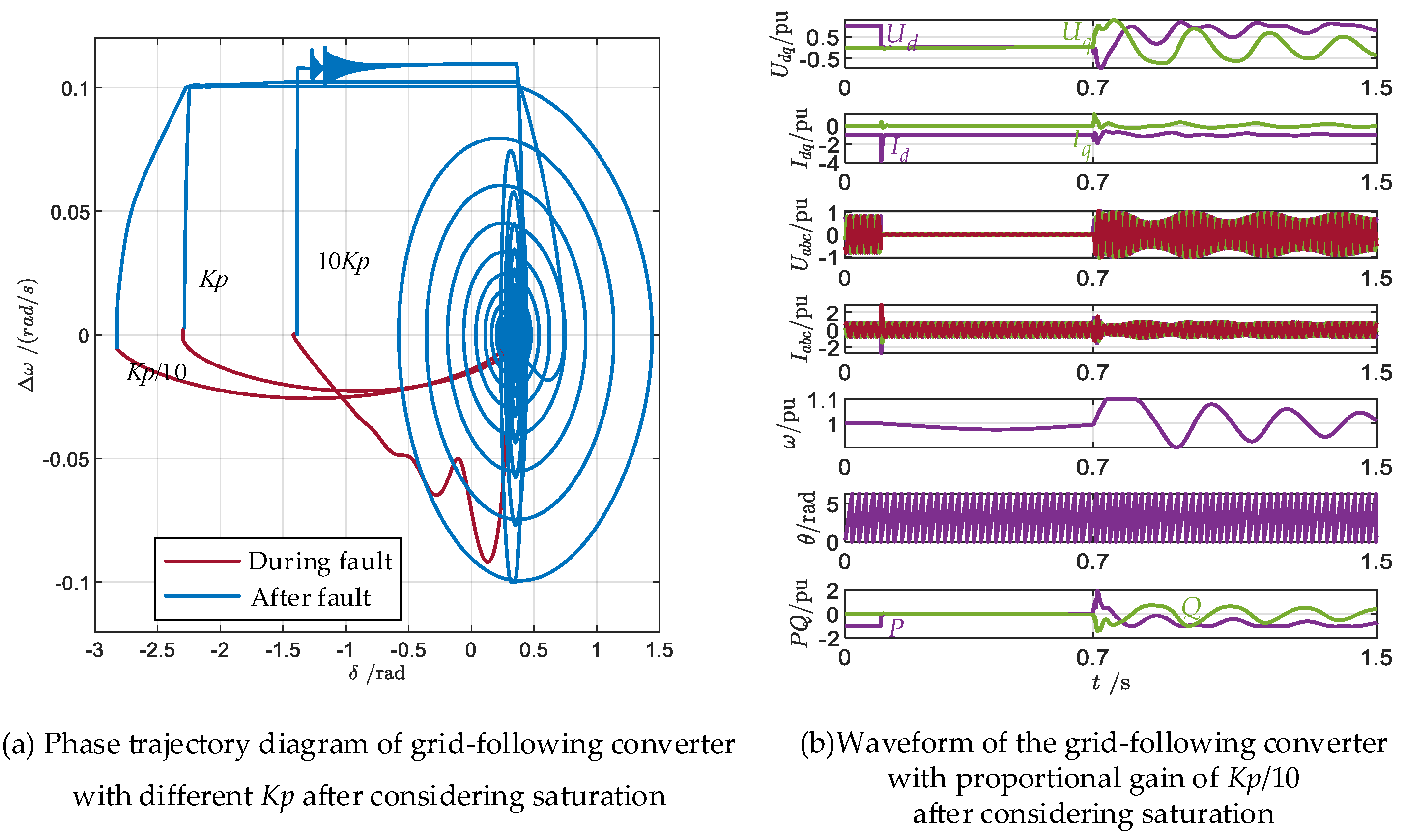
5.1. The Stability of Renewable Energy Sources Connected to the Grid under the Limitation Effect

We considered adding current amplitude and frequency limitations to the infinite system of single-phase grid-connected inverters constructed in Section 4.1. We set the output frequency of the phase-locked loop to be limited between around 0.9 and 1.1 p.u., and the output dq-axis current frequency to be limited between around −1.5 and 1.5 p.u. The integral gains of the phase-locked loop were K_I/7, KI, and 7K_I, respectively. Similarly, a three-phase short-circuit fault with a duration of 0.6 s was set near the grid-connected port of the inverter. The phase trajectory diagram of the grid-connected inverter considering the limitation effect was obtained, as shown in Figure 8a.

Comparing with Figure 5a, it can be observed that after adding the saturation element, the system could achieve stability with an integral gain of 7K_I after the fault was cleared. From Figure 8b, it can be seen that the setting of the phase-locked loop frequency limitation played a major role. Combining Figure 8a,b, it can be concluded that the frequency limitation element restricted the irreversible increase in output frequency, thus improving the stability of the system.

Similarly, the proportional gain of the phase-locked loop was made to be K_P/10, K_P, and 10K_P under the limiting link, and its phase trajectory was plotted, as in Figure 9a. Comparing with Figure 6a, it can be observed that the phase trajectory with a proportional gain of K_P/10 converged to the initial equilibrium point and no longer diverged. From Figure 9b, it can be seen that frequency limitation helped to improve the stability of grid-forming renewable energy power sources.

Due to the similar external circuit characteristics of grid-connected inverters to current sources, they have strong current support capability and rarely experience current limit exceedance during faults. Therefore, the current limitation element has little effect on grid-following inverters. The limitation elements in Figure 8b and Figure 9b also reflect the current support capability of grid-following renewable energy power sources. Therefore, the presence of frequency amplitude limiting in the grid-connected new energy power supply enhanced its transient synchronizing stability, while current amplitude limiting had minimal impact on its transient synchronizing stability.

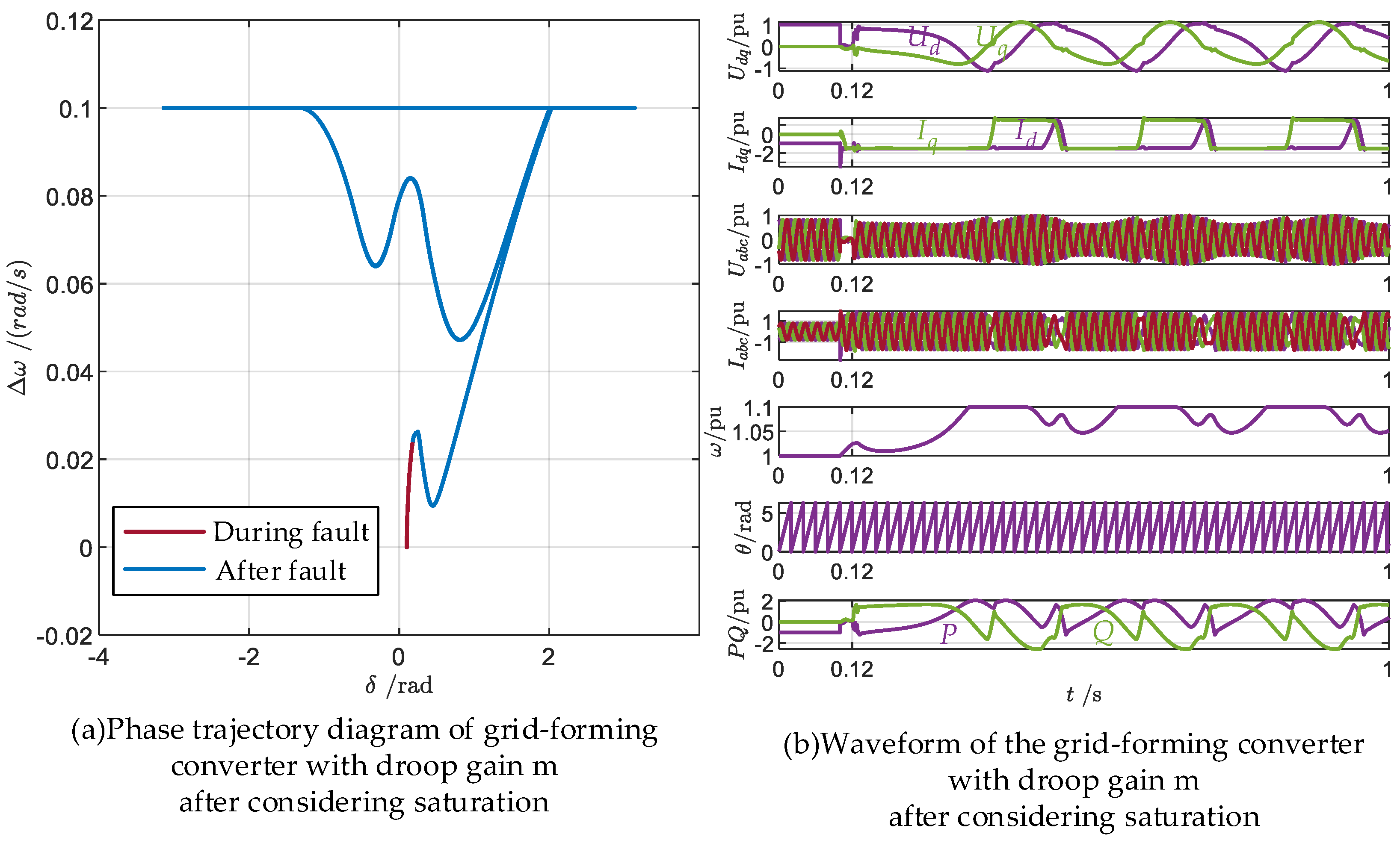
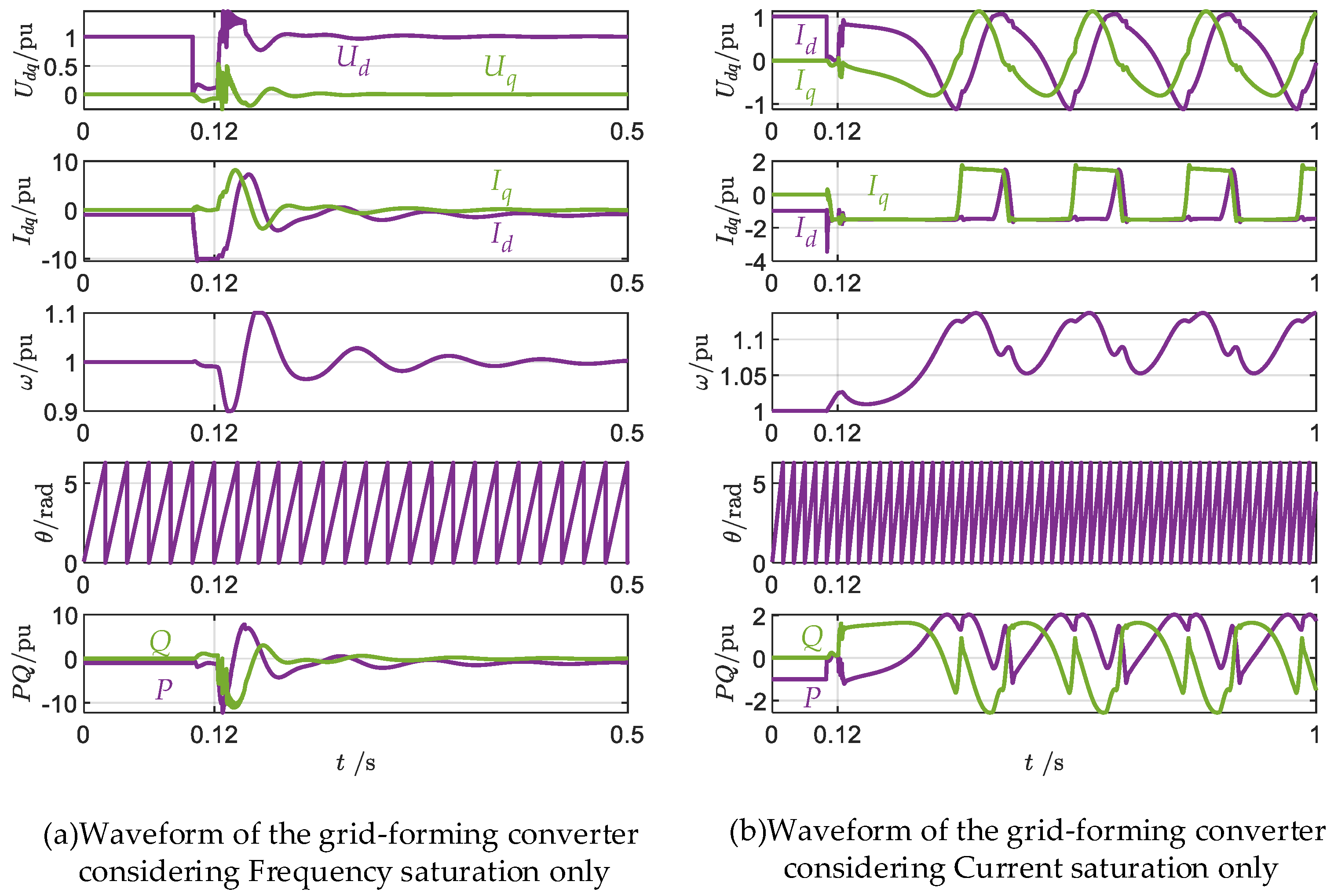
5.2. Stability of Grid-Forming Renewable Energy Power Sources under the Action of Limitation Elements

Considering the droop gain as m, the saturation parameters of each loop in the inverter were set. The output frequency of the active power droop control loop of the inverter was limited to 0.9~1.1 p.u., and the output current of the dq-axis of the inverter current loop was limited to −1.5~1.5 p.u. The dq-axis voltage of the voltage loop was also limited to −1.5~1.5 p.u. Other operating conditions were the same as the previous discussion on the infinite system of stand-alone inverters. At 0.1 s, a three-phase short-circuit fault occurred at the outlet of the inverter, and the fault duration was 0.02 s. The waveform diagram of each electrical quantity under this state was obtained, as shown in Figure 10.

It can be seen that under the consideration of limitation elements, the output current and frequency of the inverter were both limited. By comparing the current, I_abc, it can be observed that the grid-forming inverter had a significantly reduced ability to support the current, and the current exhibited more pronounced fluctuations. On the other hand, the voltage, U_abc, during the fault period had a smaller fluctuation amplitude in the grid-forming inverter compared to the grid-following inverter, which reflects the voltage source characteristics of the grid-forming inverter.

After the fault was cleared, the system transitioned from non-periodic oscillation to periodic oscillation. Under these operating conditions, we considered changing some conditions of the system to investigate their impact on the stability of the grid-connected inverter.

(1)

Different limitation conditions

From the time-domain simulation plot in Figure 10b, it can be observed that when the droop gain was set to m, considering the influence of the amplitude-limiting section, both current and frequency reached saturation. Therefore, the combined effect of the two amplitude-limiting sections cannot intuitively demonstrate their impact on transient synchronization stability. Consequently, individual simulations were conducted with separate current and frequency amplitude-limiting sections to observe their effects on transient synchronization stability, as shown in Figure 11. The time-domain simulation plots in Figure 11a show that with only the frequency amplitude-limiting section considered, the system gradually returned to stability after disturbance. Conversely, with only the current amplitude-limiting section considered, as shown in Figure 11b, the system remained unstable after disturbance. Comparing Figure 11a,b, it can be observed that the frequency amplitude-limiting section enhanced the stability of grid-connected renewable energy sources, while the current amplitude-limiting section tended to destabilize them.

(2)

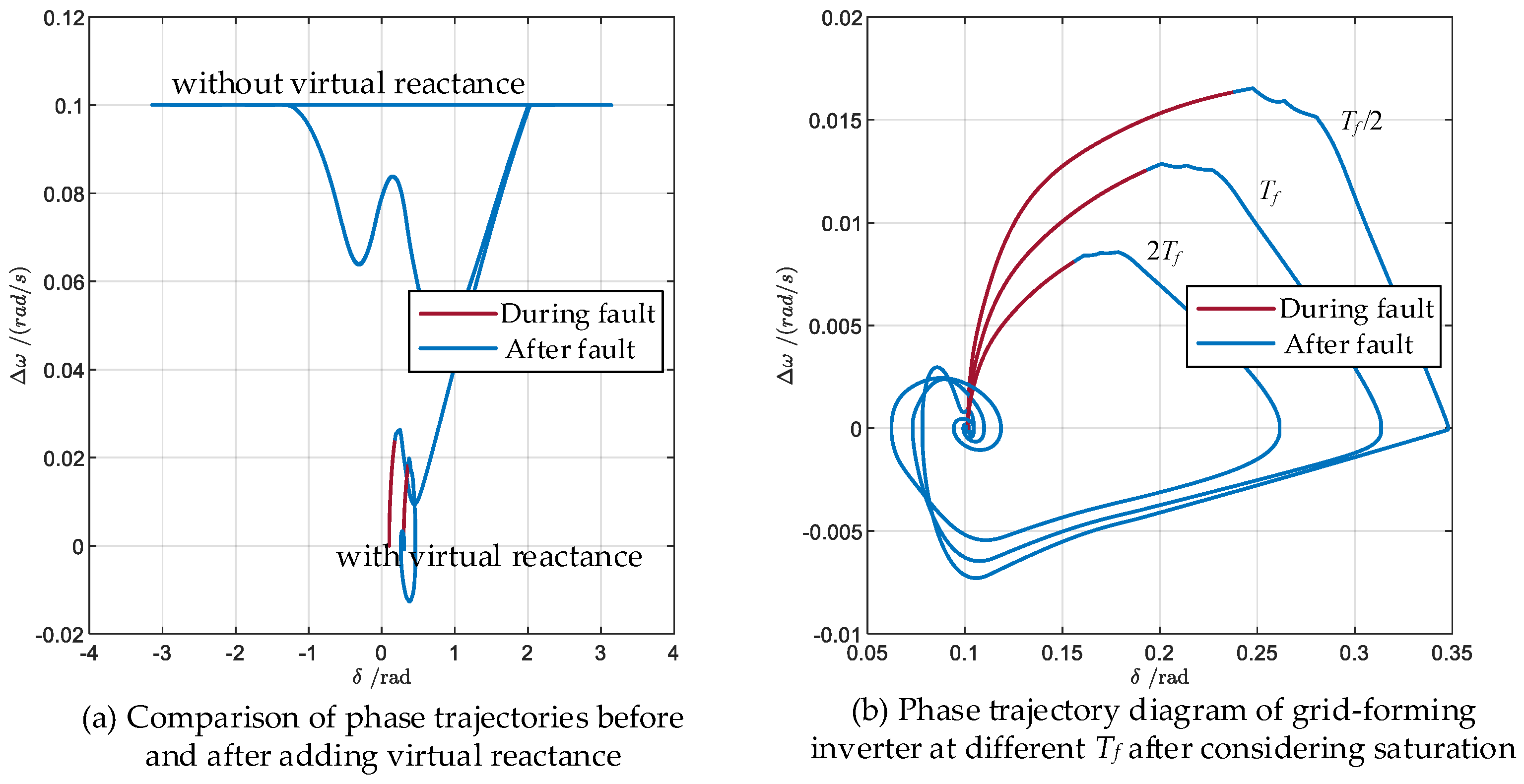
Grid-side virtual reactance of the inverter

Considering setting a virtual reactance of 0.2 p.u. on the grid side of the inverter, Figure 12a shows the phase diagram of the inverter’s output frequency and output angle with and without the virtual reactance. Without considering the virtual reactance, the frequency remained at 1.1 p.u. and the angle oscillated between -π and π. However, with the virtual reactance, the system was able to reach the original steady state after following a certain trajectory. Adding the virtual reactance is equivalent to increasing the grid impedance. These results indicate that the grid-connected inverter, controlled as a voltage source, was more prone to oscillation instability under strong grid conditions.

(3)

The time constant, T_f, of the low-pass filter

Considering the limiting loop, changing the time constant, T_f, of the low-pass filter, the phase trajectory diagram of the converter can be obtained, as shown in Figure 12b. It can be seen from the figure that as T_f increased, the variation range of the phase trajectory decreased, and the system tended to stabilize. In Figure 4b, it is shown that the increase in T_f will improve the inertia of the converter and make the system stabilize. This is consistent with the simulation results presented in Figure 12b.

The previous text discussed the impact of control parameters within the synchronous loop on the system’s synchronization stability. Changes in the control parameters will have a direct impact on the stability of the system. Based on this influence, guidance can be provided for the parameter design of converters, making their performance more superior.

When designing the control parameters of the converter’s synchronization loop, two principles are usually considered: (1) effectively suppressing high-frequency harmonics, and (2) having a sufficient phase margin. By integrating these principles, an optimal parameter selection range can be obtained. Building upon this foundation, a new principle can be introduced: having better transient synchronization stability.

In the context of grid-following converters, the authors of [29] offered an analysis focused on curbing high-frequency voltage harmonics and taking into account the phase angle margin. This analysis established the boundary constraints for the internal control parameters of the phase-locked loop (PLL). Within this constraint range, based on the conclusions drawn in the previous text, selecting a smaller K_IPLL and a larger K_pPLL can make the grid-following converter more likely to be stable.

For grid-forming converters, refer to [30] to start from the perspective of suppressing high-frequency components in the converter’s power and considering the power loop phase angle margin. The selection range for the time constant, Tf, of the droop control can be obtained. Within this range, a larger Tf can be considered, making the grid-forming converter have better transient synchronization stability.

5.3. Comparison and Summary of Characteristics of Grid-Following and Grid-Forming New Energy Sources

Through the analysis of the control structure and transient synchronous stability model of grid-following and grid-forming renewable energy sources, along with the influencing factors, it can be observed that there are many similarities between grid-following and grid-forming renewable energy sources. Summarizing this analysis yielded the following

Table 1. Comparison and summary of GFL and GFM new energy power sources.

		PLL Grid-Following Converter	Frequency Droop Grid-Forming Converter
Synchronization method		Vq-PLL by phase-locked loop	P-$\omega$ droop control
External characteristics		Current source (grid voltage-following, current-forming)	Voltage source (grid current-following, voltage-forming)
Influencing Factors	Synchronization loop control Parameters	Increasing KIPLL tends to make the system unstable. Increasing KpPLL increases system damping and reduces inertia, impacting system stability in a nonlinear relationship.	Increasing m leads the system toward instability. Increasing Tf leads the system toward stability.
	Grid strength	Stable when the grid is strong.	Stable when the grid is weak.
	Current and frequency limitations	Current limitation has little impact on stability. Frequency limition makes the system more stable.	Current limition reduces the stability region of the system. Frequency limition makes the system more stable.

.

6. Conclusions and Prospects

6.1. Conclusions

The development of new power systems led by renewable energy sources will gradually replace traditional power systems dominated by synchronous machines. It is of great significance to study the stability of grid-connected systems with renewable energy sources. The grid-connected and grid-forming renewable energy sources have a dual relationship in many respects, but there are also differences in certain aspects. This paper mainly concludes by comparing and analyzing the second-order equations that characterize the dynamic behavior of these two types of renewable energy sources.

(1) For grid-forming renewable energy sources, as the droop gain, m, increased, the equivalent inertia coefficient and damping coefficient decreased, resulting in poorer stability of the inverter. A larger time constant, Tf, of the low-pass filter led to larger equivalent inertia coefficient and damping coefficient of the inverter, resulting in better stability.

(2) For grid-following renewable energy sources, as the integral gain, KI, of the phase-locked loop increased, the equivalent inertia coefficient and damping coefficient of the inverter decreased, resulting in poorer stability of the inverter. Increasing the proportional gain, KP, of the phase-locked loop led to an increase in the equivalent damping coefficient and a decrease in the equivalent inertia coefficient of the inverter, resulting in a faster system response but a poorer disturbance rejection capability, making the system more prone to oscillations after disturbances occurred.

(3) Compared to grid-following renewable energy sources, grid-forming renewable energy sources were more prone to instability in a weak grid, while grid-following sources were more likely to experience instability in a strong grid. Correspondingly, grid-following renewable energy sources had stronger current support capabilities, which manifested as current source characteristics, while grid-forming renewable energy sources had stronger voltage support capabilities, which manifested as voltage source characteristics.

(4) Due to the nature of the grid-following inverter as a controlled current source, frequency limitation had a greater impact on its stability compared to current limitation. Adding a frequency limitation component was more beneficial for improving the stability of the grid-following inverter.

6.2. Prospects

This study contributed to explaining how instability arises when integrating new energy sources into the grid and suggested measures to mitigate such instability. However, further research and exploration are needed to comprehensively address and manage system stability concerns. For instance:

(1)

The research primarily focused on the impact of internal synchronization loops of new energy sources on their stability. However, new energy sources involve numerous control loops, and the coupling effects among these control loops are likely to influence synchronization stability.

(2)

The study only reflected trends of certain influencing factors on system synchronization stability and did not quantitatively measure the magnitude of these effects.

(3)

The investigation was confined to the transient synchronization stability of individual new energy sources integrated into the grid. However, with the increasing proportions of new energy sources, power electronic devices, and advancements in new power system configurations, the transient instability phenomena faced by future systems will become more complex.

References

1. Bai, J.; Xin, S.; Liu, J.; Zheng, K. Roadmap of Realizing the High Penetration Renewable Energy in China. Proc. CSEE 2015, 35, 3699–3705. [Google Scholar] [CrossRef]
2. Xie, X.; He, J.; Mao, H.; Li, H. New Issues and Classification of Power System Stability with High Shares of Renewables and Power Electronics. Proc. CSEE 2021, 41, 461–475. [Google Scholar] [CrossRef]
3. Zheng, X. Three Technical Challenges Faced by Power Grids with High Proportion of Non-Synchronous Machine Sources. South. Power Syst. Technol. 2020, 14, 1–9. [Google Scholar] [CrossRef]
4. Lew, D.; Bartlett, D.; Groom, A.; Jorgensen, P.; O’Sullivan, J.; Quint, R.; Rew, B.; Rockwell, B.; Sharma, S.; Stenclik, D. Secrets of Successful Integration: Operating Experience with High Levels of Variable, Inverter-Based Generation. IEEE Power Energy Mag. 2019, 17, 24–34. [Google Scholar] [CrossRef]
5. Wang, X.; Taul, M.G.; Wu, H.; Liao, Y.; Blaabjerg, F.; Harnefors, L. Grid-Synchronization Stability of Converter-Based Resources—An Overview. IEEE Open J. Ind. Appl. 2020, 1, 115–134. [Google Scholar] [CrossRef]
6. Rosso, R.; Wang, X.; Liserre, M.; Lu, X.; Engelken, S. Grid-Forming Converters: Control Approaches, Grid-Synchronization, and Future Trends—A Review. IEEE Open J. Ind. Appl. 2021, 2, 93–109. [Google Scholar] [CrossRef]
7. Chi, Y.N.; Jiang, B.W.; Hu, J.B.; Lin, W.F.; Liu, H.Z.; Fan, Y.W.; Ma, S.C.; Yao, J. Grid-forming Converters: Physical Mechanism and Characteristics. High Volt. Eng. 2024, 50, 590–604. [Google Scholar] [CrossRef]
8. Du, W.; Tuffner, F.K.; Schneider, K.P.; Lasseter, R.H.; Xie, J.; Chen, Z.; Bhattarai, B. Modeling of Grid-Forming and Grid-Following Inverters for Dynamic Simulation of Large-Scale Distribution Systems. IEEE Trans. Power Deliv. 2021, 36, 2035–2045. [Google Scholar] [CrossRef]
9. Li, M.; Zhang, X.; Guo, Z.; Pan, H.; Ma, M.; Zhao, W. Impedance Adaptive Dual-Mode Control of Grid-Connected Inverters with Large Fluctuation of SCR and Its Stability Analysis Based on D-Partition Method. IEEE Trans. Power Electron. 2021, 36, 14420–14435. [Google Scholar] [CrossRef]
10. Kez, D.A.; Foley, A.M.; Morrow, D.J. Analysis of Fast Frequency Response Allocations in Power Systems with High System Non-Synchronous Penetrations. IEEE Trans. Ind. Appl. 2022, 58, 3087–3101. [Google Scholar] [CrossRef]
11. Taul, M.G.; Wang, X.; Davari, P.; Blaabjerg, F. An Overview of Assessment Methods for Synchronization Stability of Grid-Connected Converters Under Severe Symmetrical Grid Faults. IEEE Trans. Power Electron. 2019, 34, 9655–9670. [Google Scholar] [CrossRef]
12. Li, Y.; Gu, Y.; Green, T.C. Revisiting Grid-Forming and Grid-Following Inverters: A Duality Theory. IEEE Trans. Power Syst. 2022, 37, 4541–4554. [Google Scholar] [CrossRef]
13. Liu, Z.X.; Qin, L.; Yang, S.Q.; Zhou, Y.Y.; Wang, Q.; Zheng, J.W.; Liu, K.P. Review on Virtual Synchronous Generator Control Technology of PowerElectronic Converter in Power System Based on New Energy. Power Syst. Technol. 2023, 47, 1–16. [Google Scholar] [CrossRef]
14. Tan, S.; Geng, H.; Yang, G. Phillips-Heffron model for current-controlled power electronic generation unit. J. Mod. Power Syst. Clean Energy 2017, 6, 582–594. [Google Scholar] [CrossRef]
15. Zheng, X. Physical mechanism and research approach of generalized synchronous stability for power systems. Electr. Power Autom. Equip. 2020, 40, 3–9. [Google Scholar] [CrossRef]
16. Haoyue, G.; Qiang, G.; Jianbo, G.; Qinyong, Z.; Jian, Z.; Libo, Z.; Lei, G. Small Disturbance Stability Analysis and Control Research Based on State Space Method of Converter System. Proc. CSEE 2024, 1–16. [Google Scholar]
17. Yan, W.B.; Huang, Y.H.; Fang, Z.; Wang, D.; Tang, J.R.; Zhou, K.L. Stability Mechanism Analysis of Grid-forming Converter Connected to Low Impedance Grid. High Volt. Eng. 2024, 1–12. [Google Scholar] [CrossRef]
18. Wang, X.; Harnefors, L.; Blaabjerg, F. Unified Impedance Model of Grid-Connected Voltage-Source Converters. IEEE Trans. Power Electron. 2018, 33, 1775–1787. [Google Scholar] [CrossRef]
19. Huang, L.L.; Xin, H.H.; Ju, P.; Hu, J.B. Synchronization stability analysis and unified synchronization control structure of grid-connected power electronic devices. Electr. Power Autom. Equip. 2020, 40, 10–25. [Google Scholar] [CrossRef]
20. Zou, Z.Y.; Wu, C.; Wang, Y.; Tian, J.; Zhan, C.J. Transient Stability Analysis of Islanded System with Parallel Grid-forming Converters Based on Equivalent Synchronous Power. Autom. Electr. Power Syst. 2024, 48, 140–150. [Google Scholar]
21. Zhang, L.Q.; Liu, Y.; Xin, H. Phase-plane analyses of a microgrid under PQ control mode. In Proceedings of the International Conference on Sustainable Power Generation and Supply (SUPERGEN 2012), Hangzhou, China, 8–9 September 2012. [Google Scholar]
22. Shuai, Z.; Shen, C.; Liu, X.; Li, Z.; Shen, Z.J. Transient Angle Stability of Virtual Synchronous Generators Using Lyapunov’s Direct Method. IEEE Trans. Smart Grid 2019, 10, 4648–4661. [Google Scholar] [CrossRef]
23. Wu, H.; Wang, X. Design-Oriented Transient Stability Analysis of PLL-Synchronized Voltage-Source Converters. IEEE Trans. Power Electron. 2020, 35, 3573–3589. [Google Scholar] [CrossRef]
24. Hu, Q.; Fu, L.; Ma, F.; Ji, F. Large Signal Synchronizing Instability of PLL-Based VSC Connected to Weak AC Grid. IEEE Trans. Power Syst. 2019, 34, 3220–3229. [Google Scholar] [CrossRef]
25. Chen, J.; Liu, M.; O’Donnell, T.; Milano, F. Impact of Current Transients on the Synchronization Stability Assessment of Grid-Feeding Converters. IEEE Trans. Power Syst. 2020, 35, 4131–4134. [Google Scholar] [CrossRef]
26. Cecati, C.; Latafat, H. Time domain approach compared with direct method of Lyapunov for transient stability analysis of controlled power system. In Proceedings of the International Symposium on Power Electronics, Sorrento, Italy, 20–22 June 2012. [Google Scholar]
27. Yuan, X.M.; Zhang, M.Q.; Chi, Y.N.; Ju, P. Basic Challenges of and Technical Roadmap to Power-electronized Power System Dynamics Issues. Proc. CSEE 2022, 42, 1904–1917. [Google Scholar] [CrossRef]
28. Li, Y. Modeling and Control of Power Electronic Converter. Ph.D. Thesis, Imperial College London, London, UK, 2020. [Google Scholar]
29. Yan, P.L.; Ge, X.L.; Wang, H.M.; Sun, W.X.; Zhu, Y.L. PLL Parameter Optimization Design for Renewable Energy Grid-connected Inverters in Weak Grid. Power Syst. Technol. 2022, 46, 2210–2221. [Google Scholar] [CrossRef]
30. Wu, H.; Ruan, X.B.; Yang, D.S.; Chen, X.R.; Zhong, Q.C.; Lv, Z.P. Modeling of the Power Loop and Parameter Design of Virtual Synchronous Generators. Proc. CSEE 2015, 35, 6508–6518. [Google Scholar] [CrossRef]
Figure 1. Grid-following inverter. (a) Grid-following inverter control structure. (b) Phase-locked loop control.
Electronics 13 03308 g001
Figure 2. Grid-forming inverter. (a) Grid-forming inverter control structure. (b) Droop control with LPF structure.
Electronics 13 03308 g002
Figure 3. Comparison of control block diagrams for three nonlinear dynamic equations. (a) Synchronous generator. (b) Grid-following inverter. (c) Grid-forming inverter.
Electronics 13 03308 g003
Figure 4. Comparison of stability-influencing factors of two new energy power sources. (a) Grid-following control. (b) Grid-forming control.
Electronics 13 03308 g004
Figure 5. Effect of KI on the stability of the grid-following inverter and waveforms after destabilization. (a) Phase trajectory after changing the KI. (b) Waveforms after destabilization.
Electronics 13 03308 g005
Figure 6. Effect of KP on the stability of the grid-following inverter and waveforms after destabilization. (a) Phase trajectory after changing the KP. (b) Waveforms after destabilization.
Electronics 13 03308 g006
Figure 7. Effect of m on the stability of the grid-forming inverter and waveforms after destabilization. (a) Phase trajectory after changing the m. (b) Waveforms after destabilization.
Electronics 13 03308 g007
Figure 8. Effect of KI on the stability of the grid-following inverter and waveforms after considering saturation. (a) Phase trajectory after changing the KI. (b) Waveforms with the integration gain of 7KI.
Electronics 13 03308 g008
Figure 9. Effect of Kp on the stability of the grid-following inverter and waveforms after considering saturation. (a) Phase trajectory after changing the Kp. (b) Waveforms with the integration gain of 7Kp.
Electronics 13 03308 g009
Figure 10. Instability diagram of the grid-forming converter considering saturation.
Electronics 13 03308 g010
Figure 11. Waveform plots of the current and frequency amplitude limitations acting separately.
Electronics 13 03308 g011
Figure 12. Influence of virtual reactance and Tf on the stability of grid-configured converters. (a) Influence of virtual reactance. (b) Influence of LPF constant (Tf).
Electronics 13 03308 g012