Abstract
Automatic emotion recognition using portable sensors is gaining attention due to its potential use in real-life scenarios. Existing studies have not explored Galvanic Skin Response and Photoplethysmography sensors exclusively for emotion recognition using nonlinear features with machine learning (ML) classifiers such as Random Forest, Support Vector Machine, Gradient Boosting Machine, K-Nearest Neighbor, and Decision Tree. In this study, we proposed a genuine window sensitivity analysis on a continuous annotation dataset to determine the window duration and percentage of overlap that optimize the classification performance using ML algorithms and nonlinear features, namely, Lyapunov Exponent, Approximate Entropy, and Poincaré indices. We found an optimum window duration of 3 s with overlap and achieved accuracies of 0.75 and 0.74 for both arousal and valence, respectively. In addition, we proposed a Strong Labeling Scheme that kept only the extreme values of the labels, which raised the accuracy score to 0.94 for arousal. Under certain conditions mentioned, traditional ML models offer a good compromise between performance and low computational cost. Our results suggest that well-known ML algorithms can still contribute to the field of emotion recognition, provided that window duration, overlap percentage, and nonlinear features are carefully selected.
1. Introduction
With the growing proliferation of wearable sensors capable of uploading biosignal data to the cloud, automatic emotion recognition has acquired significant interest due to its potential applications in education, psychology, well-being, medicine, neuroscience, driver safety, and other fields [1,2,3,4,5].
The most common biosensors are electrocardiography (ECG), respiration (RESP), electroencephalography (EEG), galvanic skin response (GSR) or electrodermal activity (EDA), electrooculography (EOG), photoplethysmography (PPG) or blood volume pulse (BVP), electromyography (EMG), and skin temperature (SKT or TEMP) [2,3]. Not all of them are comfortable, user-friendly, or portable, which makes them ill-suited to be employed outside a laboratory environment, at least with the current technological development.
Among the mentioned biosensors, Galvanic Skin Response (GSR) and Photoplethysmography (PPG) stand out as portable, non-invasive sensors capable of gathering larger volumes of data over time due to their ease of use. Although there are not many portable GSR and PPG sensors capable of collecting clinical-quality data currently, sensors with improved signal quality are expected to emerge in the future [6]. Thus, in this study, we focus on automatic emotion recognition employing only GSR and PPG biosignals. GSR sensors typically measure skin electrical conductance using two electrodes, usually placed on the fingers. Skin conductance is linked to sweating, which in turn is connected to emotions [7,8]. On the other hand, PPG sensors indirectly measure heart rate and other associated metrics, such as the average of inter-beat intervals (IBI), the standard deviation of heart rate (SDNN), and the Root Mean Square of Successive Differences (RMSSD), which are also linked to emotions [7,9]. They are typically worn on the wrist.
Emotion recognition is carried out by applying machine learning algorithms directly to the biosignals or some set of extracted features when an individual is subjected to some affect elicitation stimulus (e.g., video clips and images) [3]. The individual usually annotates emotions subjectively on a two-dimensional model using two continuous scales, i.e., valence and arousal, typically ranging from 1 to 9. Valence denotes how pleasant or unpleasant the emotion is, while arousal represents the intensity [3]. Valence and arousal are usually treated as two independent classification problems [10].
Additionally, data annotation can be discrete or continuous [11,12,13,14]. In the former case, labels are recorded in an indirect, post-hoc manner, e.g., one label is annotated after a video clip of 60 s is shown. In the latter case, data labels are annotated with higher frequencies. Most publicly available datasets follow a discrete annotation paradigm with subjective methods.
The process of emotion elicitation and labeling usually takes no less than an hour per individual, including participant instruction, trials to familiarize with the system, baseline recordings, stimulus presentation, and annotations. This induces fatigue in participants. As a result, datasets typically do not have many samples per participant. This is a significant problem in the emotion recognition field but can be addressed with proper segmentation of the labels, at least until larger datasets become available.
Regarding the selection of features to extract from biosignals, there is no consensus on the optimum set that maximizes the accuracy of emotion recognition in every situation. The selection of features is typically problem-dependent [3]. Nonetheless, features from temporal, statistical, and nonlinear domains extracted from GSR and PPG signals have yielded very good results [1,15,16]. A particular challenge is finding the set that combines GSR- and PPG-extracted features to yield optimal performance.
Some existing works on emotion recognition are based solely on GSR and PPG. Martínez et al. [17] proposed a stack of two Convolutional Neural Networks (CNNs) followed by a simple perceptron to recognize discrete emotions (relaxation, anxiety, excitement, and fun) using GSR and PPG modalities from participants playing a predator/prey game. Participants annotated data in a ranking or preference-based format (e.g., “Y is funnier than W”) by filling out a comparison questionnaire in a post-hoc manner. Thus, the annotations were discrete. They found that the proposed deep learning model, which automatically and directly extracts features from the raw data, outperforms models utilizing known statistically ad-hoc extracted features, attaining an accuracy of 0.75. Ayata et al. [18] proposed a music recommendation system based on emotions using the DEAP dataset [11], which utilizes music videos to elicit emotions. Each participant rated their emotions subjectively on a 1 to 9 valence/arousal scale by answering a questionnaire after each 60 s video. Hence, only one label per dimension is available for each stimulus video, and the annotations were discrete. They achieved accuracies of 0.72 and 0.71 on arousal and valence, respectively, by feeding a Random Forest (RF) classifier with statistical features. The work studied the effect of window duration size for GSR and PPG separately and found that 3 s windows performed better for GSR while 8 s windows performed better for PPG. Kang et al. [19] presented a signals-based labeling method that involved windowing (data were window-sliced in one-pulse units) and observer-annotated data. They applied a 1D convolutional neural network to recognize emotions on the DEAP and MERTI-Apps datasets [20]. In the MERTI-Apps dataset, data were annotated objectively by five external observers every 0.25 s after watching the participant’s recorded face. In case of disagreement, a specific protocol was followed to reach a consensus label, excluding annotation inconsistencies if necessary. Despite the high data annotation frequency for a discrete annotation paradigm, the annotation method is not real-time and the labels are not subjective. They obtained accuracies of and on the MERTI-Apps dataset [20] for arousal and valence, respectively, while achieving and on arousal and valence, respectively, using the DEAP dataset.
Goshvarpour et al. [16] implemented a Probabilistic Neural Network (PNN) to recognize emotions based on nonlinear features. Approximate Entropy, Lyapunov Exponent, and Poincaré indices (PI) were extracted and fed to the PNN. They validated the experiment using the DEAP dataset and obtained and for arousal and valence, respectively. As noted in [18,19], they employed a discrete annotation method. Domínguez-Jiménez et al. [21] conducted an experiment with 37 volunteers employing wearable devices. Participants rated three discrete emotions (i.e., amusement, sadness, and neutral) in a post-stimuli survey using a 1 to 5 scale, following a discrete annotation paradigm. They were able to recognize these three emotions with an accuracy of when a linear Support Vector Machine (SVM) classifier was trained with statistical features selected by feature selection methods such as Genetic Algorithm (GA) or Random Forest Recursive Feature Selection (RF-RFE). In addition, in our previous work [22], we adopted a robust labeling scheme that discarded neutral values of valence and arousal, keeping only extreme values (i.e., ranges from [1–3] and [7–9]). As we were interested in testing the generalization skills of certain algorithms, such as SVM, K-Nearest Neighbor (KNN), and Gradient Boosting Machine (GBM), in a subject-dependent emotion classification context, we tested the same model parameters on two datasets: DEAP and K-EmoCon [13]. The former employs non-portable sensors, while the latter uses wearable sensors. In the K-EmoCon dataset, participants annotated data retrospectively every 5 s after watching their own recorded face. Consequently, we used a discrete data annotation method. We found that accuracies of 0.7 and an F1-score of 0.57 are attainable, but this comes at the expense of discarding some samples.
All of the mentioned works employ discrete labeling methods. Although some used windowing to increase the number of samples and enhance recognition performance, they often reused the same labels due to the discontinuous annotation paradigm of the datasets (e.g., multiple uses of a single label from a 60 s video clip). As a result, local emotional changes are missed or filtered out because participants can only rate their emotions at specific intervals. Therefore, a genuine windowing method based solely on GSR and PPG sensors needs to be included in the literature. This study addresses this gap by employing a continuous, real-time annotation dataset. The purpose of this decision is twofold: to use a greater number of samples in the model’s training and to perform genuine window segmentation on the data and annotations, allowing for better capture of local emotional changes with varying window durations. To the best of our knowledge, no authentic window sensitivity study has been performed on a continuous annotation dataset using only the two mentioned sensors. This sensitivity study is relevant for determining the optimal window duration and percentage of overlap that best capture elicited emotions at the precise moment the individual feels them and within the appropriate time interval. It is important to note that several factors justify this approach:
- The duration of emotions is highly variable; therefore, the optimal window duration strongly depends on how the individual labels the elicited emotions.
- Within a given window, the individual can significantly change the label (due to the continuous nature of the dataset). Therefore, small window sizes can potentially capture ‘local variations’ but are more susceptible to capturing label artifacts, which may confuse the classifier. On the other hand, large window sizes combined with an appropriate metric condensing the participant’s annotation of the entire segment can filter out these label artifacts and capture more emotional information. However, this metric may be unsuitable if label fluctuations are significant. An optimal window duration can both filter out label artifacts and keep the metric representative of the labels within the segment.
- The representative metric of a consecutive overlapped window can better capture local emotional fluctuations that might be filtered out by the metric of the previous window (e.g., if the fluctuations occur at the end of the previous window).
Therefore, the main contribution of this work is the sensitivity analysis of the window size. Consequently, we conducted a sensitivity study on window duration size and percentage overlap to identify the optimal values that result in better recognition performance. Additionally, we compared the performance of temporal–statistical and nonlinear features. Moreover, different labeling schemes were adopted to explore how accuracy increased as the thresholds for label binarization were raised. Finally, the main aim of our work was to find the window duration size and percentage of overlap that optimized emotion recognition performance using only GSR and PPG while employing low-computational-cost algorithms. We found that this can be accomplished provided that data annotation is continuous and nonlinear features are used.
2. Materials and Methods
To conduct this study, we employed the CASE dataset [14], which features continuous annotations sampled at 20 Hz. Each participant was subjected to 8 film clips, each lasting 1.5 to 3.5 min. During the stimulus, the participant annotated the video on a 2D plane in real-time. The axes of the plane are valence and arousal. A total of 30 participants participated in the experiment, 15 male and 15 female.
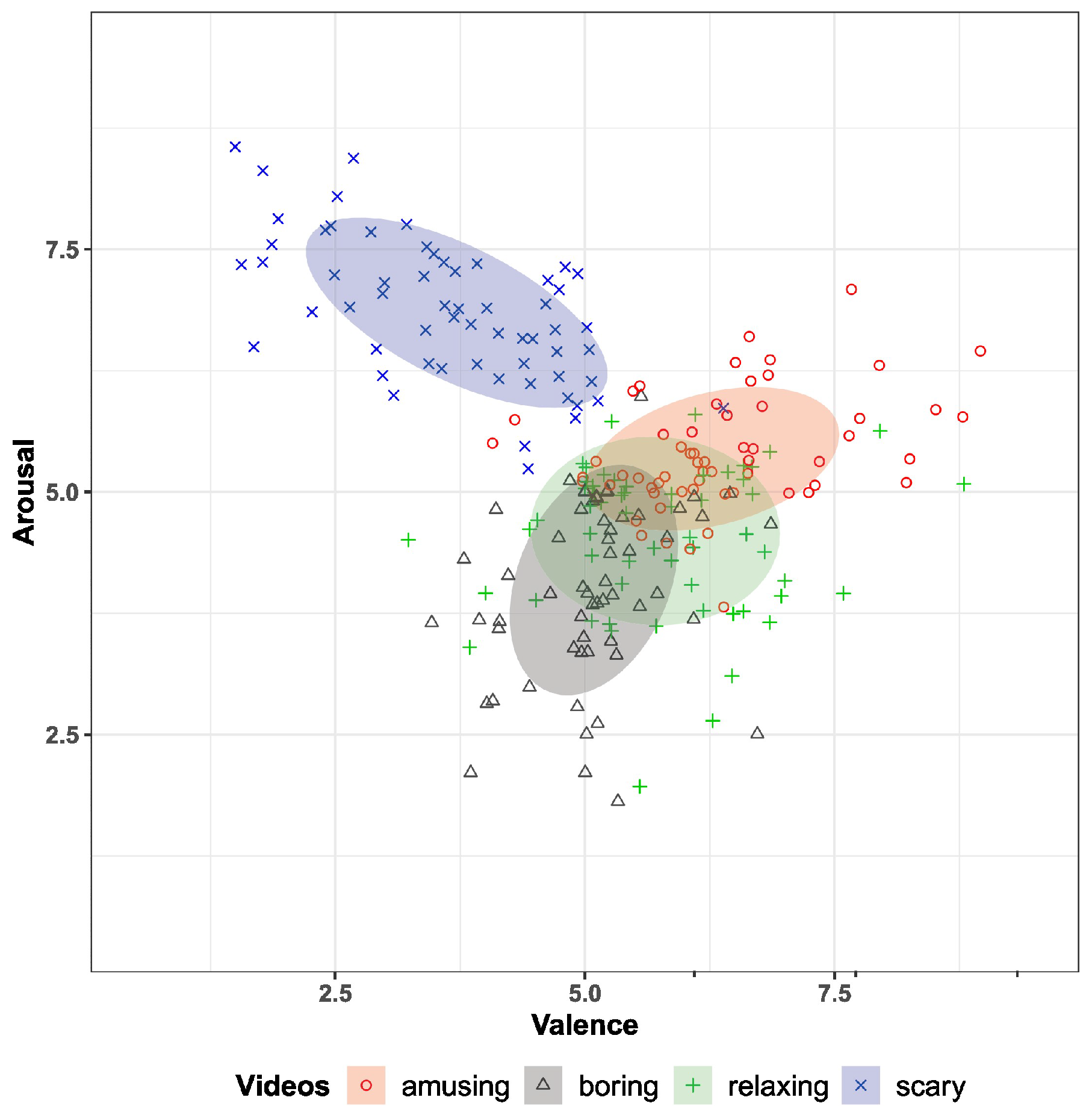
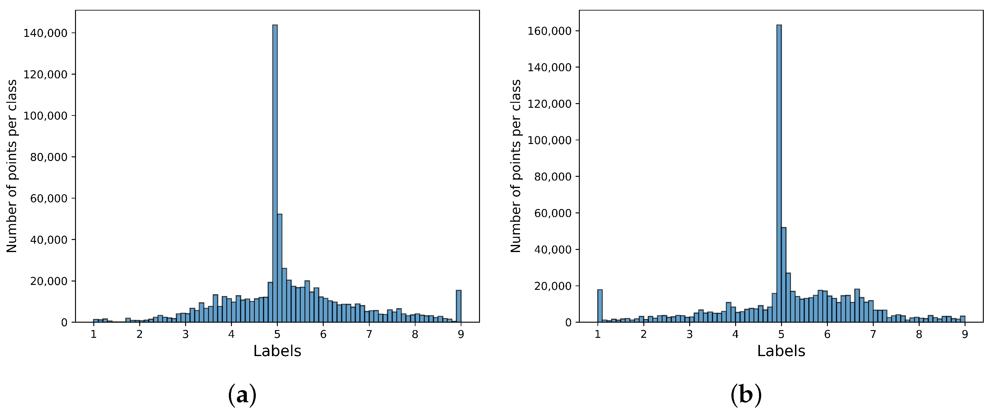
The annotations were made using a joystick-based interface to rate each stimulus video on the valence and arousal continuous scale, ranging from 1 to 9. Each individual subjectively rated their emotions in real-time while watching each video. The mean distribution of the labels can be seen in Figure 1. Each point in the scatter plot represents the mean label for a specific video, annotated by a participant. A total of 240 points are displayed (30 participants × 8 videos per participant). On the other hand, the number of points for each class can be seen in Figure 2. Each point corresponds to a particular sample from the joystick-based sensors, with a sample period of ms. GSR and PPG raw data were sampled at 1000 Hz.

Figure 1.
Scatter plot of the mean annotation data, labeled according to the types of videos (each point corresponds to a video clip). Adapted from “A dataset of continuous affect annotations and physiological signals for emotion analysis” by [14]. Licensed under a Creative Commons Attribution 4.0 International License. Changes made: cropped the scatter plot and centered the legends for the video types in this figure. https://www.nature.com/articles/s41597-019-0209-0 (accessed on 1 August 2024).
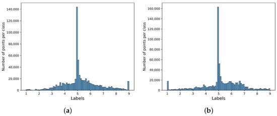
Figure 2.
Number of points for each class in the CASE dataset. The label range from 1 to 9 was split into data bins of 0.1. (a) Arousal. (b) Valence.
For each participant, the experiment was conducted in the following order: first, a relaxing start video was shown to calm the participants before the presentation; then, a transitioning blue screen was displayed, followed by a stimulus video. This sequence of the blue screen followed by the stimulus video was repeated 8 times. Biosignals were collected from the moment the start video was shown.
2.1. Data Preprocessing
We made use of linear interpolated data and annotations to mitigate data latency issues that occurred during data acquisition, ensuring they were effectively sampled at regular intervals of 1 ms and 50 ms, respectively [14]. Subsequently, we applied a baseline mean-centered normalization, as suggested by [15], following this equation:
where is the raw signal and represents the signal acquired during the last 60 s of the start video [14]. After normalization, we applied a fourth-order Butterworth low-pass filter with a cut-off frequency of 3 Hz to the GSR signal and a third-order Butterworth band-pass filter with cutoff frequencies of 0.5–8 Hz to the PPG signal, using the Neurokit package [23].
To test the effects of window duration and percentage of overlap, we segmented the data and continuous labels into various window sizes ( s) and overlap percentages (). We selected these ranges based on [7,18,24]. Ref. [7] reported several studies employing films as the eliciting stimulus with window durations ranging from 0.5 to 120 s. Ref. [18] utilized window sizes from 1 to 30 s, but with non-uniform steps and decreasing accuracy for s. Ref. [24] employed window durations ranging from 0.125 to 16 s, with non-uniform steps, and reported poor performance for s. Therefore, we chose to use a uniform step size ranging from 1 to 29 s to facilitate the identification of the optimal window size. Before segmentation, annotations were upsampled to match the sample rate of the PPG and GSR signals.
2.2. Labels Mapping
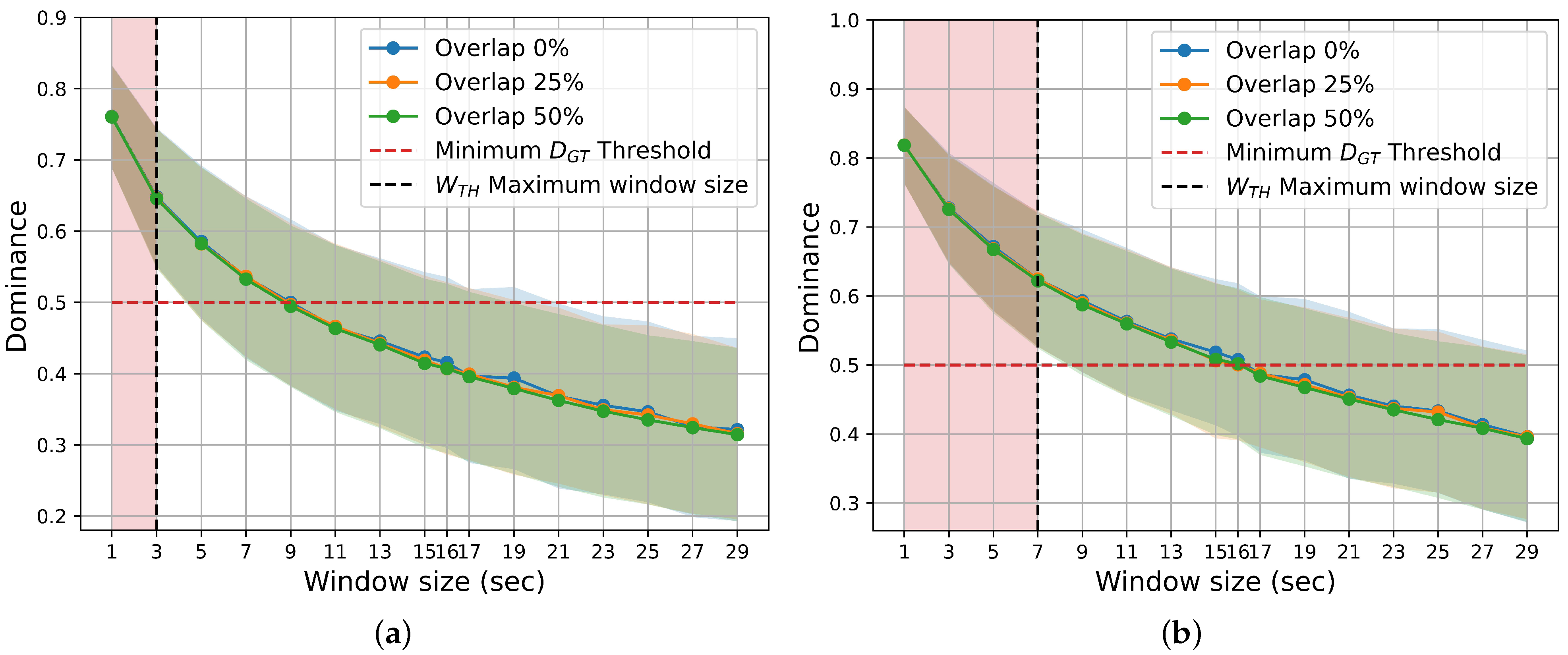
Because data labels are continuous and can vary within a given segment, each annotation segment should be replaced by a particular value to train different models and make classification possible. We replaced each segment with its median value. This method avoids discarding segments, which was a premise of this work, given the low number of data samples available (e.g., less than 250 instances for a s and ). Moreover, we found it more convenient not to discard segments a priori in order to perform the window sensitivity analysis for all the proposed window sizes. To ensure that the median is representative of the annotation segment, we should choose a dominance ground truth (GT) label’s minimum threshold of or higher. Dominance is calculated as follows:
where represents the percentage of the label within a window instance. We chose the minimum ground truth threshold to be . Once we determined the change in the GT label percentage across different window sizes and overlap ratios, we only considered those window segments that met the criterion, based on a worst-case scenario (Note that is the standard deviation of . See Section 3).
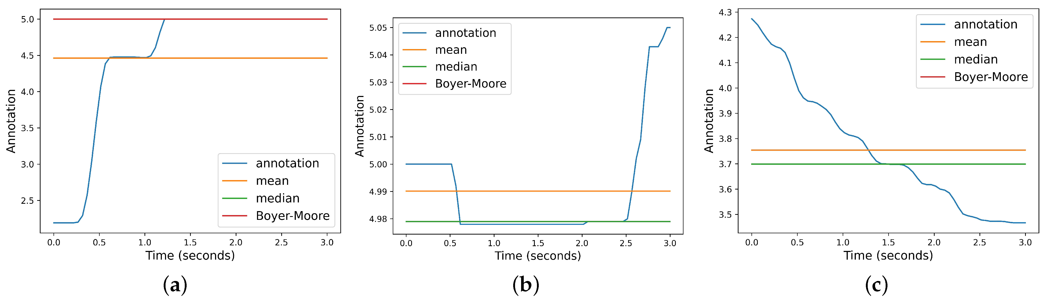
We think this method better represents user labeling than replacing the annotation segment with its mean value. If , this method yields the same results as the Boyer–Moore voting algorithm [25] but without discarding any window instances a priori. The Boyer–Moore voting algorithm is a standard majority method that only yields a result if the majority value has more than half of the total samples in the window.
When there is a clear majority in favor of a particular label, the median value aligns with the label of the longest horizontal line. In such cases, the Boyer–Moore and median methods yield the same result, while the mean may produce a different value (see Figure 3a). On the other hand, when there is no clear majority, the Boyer–Moore method does not yield a result and the mean sometimes deviates significantly from the most-selected labels, whereas the median tends to be closer to the labels corresponding to the longest horizontal subsegments, better representing the selected majority of labels for the given segment (see Figure 3b). However, we would eventually discard all window instances that do not meet the criterion when training an emotion recognition model for a particular subject in a real-life scenario. In extreme cases where no label has more more than one vote, the median and the mean yield approximately the same results (see Figure 3c). In this circumstance, neither the median method nor the Boyer–Moore algorithm would produce a representative result and would require discarding an instance, which is not desirable.
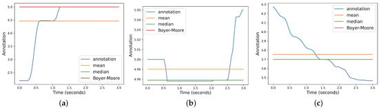
Figure 3.
Segment labels mapping: from continuous multivalued labels to one value annotation per segment. (a) Clear majority. (b) No clear majority. (c) No clear majority: extreme case.
2.3. Labeling Schemes
Once the continuous labels in a segment were replaced with its median value, a slight variant of the Bipartition Labeling Scheme (BLS) mentioned by [26] is adopted. Labels were binarized according to three different schemes: classic, weak, and strong. Each scheme is detailed in Table 1.

Table 1.
Labeling schemes.
2.4. Data Splitting
To handle imbalanced data and avoid artifacts that may arise from the way the training and test datasets are organized, we applied a stratified K-Fold cross-validation strategy with 10 folds. We computed metrics for each hold-out test set and averaged them over the 10 scores to determine the participant’s emotion recognition performance (see Section 2.6). This method allows us to demonstrate the intrinsic relationship between the window settings and the machine learning techniques.
2.5. Feature Extraction
Based on the good results and methodology described in [16], we extracted several nonlinear features for GSR and PPG, as these signals exhibit chaotic and nonlinear behaviors. Specifically, we extracted Approximate Entropy (ApEn), Lyapunov Exponent (LE), and some Poincaré indices (PI). While ApEn measures the complexity or irregularity of a signal [16], the LE of a time series indicates whether the signal presents chaotic behavior or, conversely, has a stable attractor. On the other hand, specific indices from Lagged Poincaré Plots quantify the PPG and GSR attractors. The extracted features can be seen in Table 2.
Table 2.
Extracted nonlinear features from Galvanic Skin Response (GSR) and Photoplethysmography Signals (PPG).
A total of 20 nonlinear features were extracted for each window segment: 10 for GSR and 10 for PPG. These features are LE, ApEn, SD11, SD21, SD121, S1, SD110, SD210, SD1210, and S10.
To compare the ability to extract relevant information from the physiological signals between two different feature extraction domains, well-known temporal–statistical features were also extracted, as shown in Table 3.
Table 3.
Extracted temporal–statistical features from GSR and PPG.
A total of 8 temporal–statistical features were extracted for each window segment: 3 for GSR and 5 for PPG.
Additionally, features from the GSR and PPG sensors were standardized using the following equation:
where is the standard deviation. Finally, standardization was fitted on the training dataset and applied to the training and testing datasets.
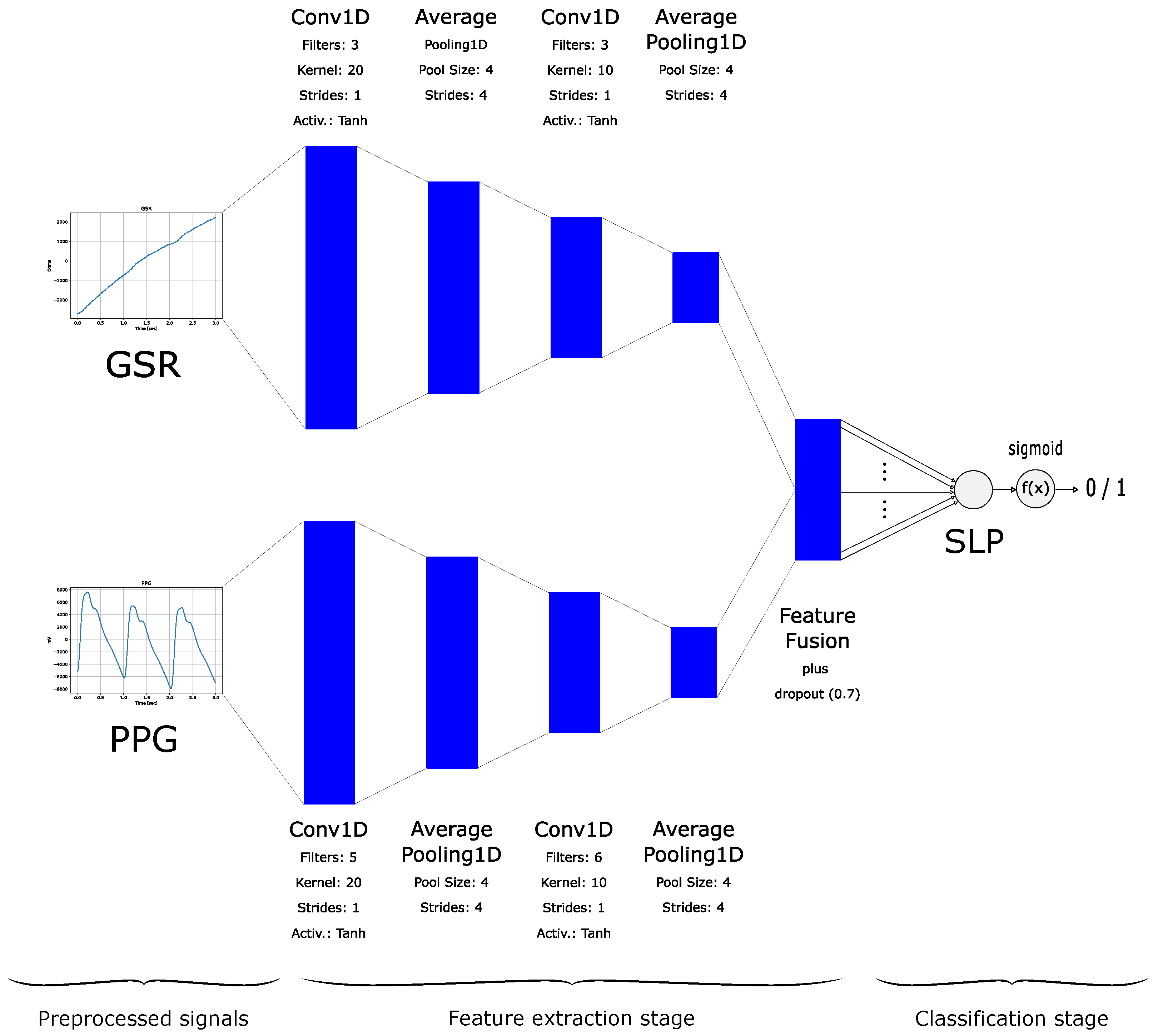
For comparison purposes, we also trained a Convolutional Neural Network with a Single-Layer Perceptron Classifier (CNN-SLP) algorithm, as detailed in [22]. The CNN-SLP is a variation of the model proposed by [17]. It automatically extracts features directly from the GSR and PPG time series, following a representation learning paradigm [30]. These learned features from PPG and GSR are fused into a unified vector, which serves as the input for a Single-Layer Perceptron classifier (see Figure 4).

Figure 4.
Convolutional Neural Network with a Single-Layer Perceptron Classifier (CNN-SLP). First published in IFMBE Proceedings, Volume 1, pages 23–35, 2024 by Springer Nature [22].
2.6. Algorithm Training and Performance Evaluation
In this study, six algorithms were trained: Decision Tree (DT), KNN, RF, SVM, GBM, and CNN-SLP. Except for the latter, all other algorithms can be considered shallow learning models [31].
As we were interested in performing a subject-dependent emotion classification [3], and assessing the generalization ability of each algorithm, we employed the same hyperparameters utilized in [22], tested on the DEAP and K-Emocon datasets [11,13]. The set of chosen hyperparameters can be seen in Table 4.
Table 4.
Algorithms’ hyperparameters.
To assess the performance, we employed the accuracy (ACC), unweighted average recall (UAR) [32], and F1-score (F1). Both UAR and F1 are well-suited for imbalanced datasets.
Because our approach is subject-dependent emotion recognition, we computed these metrics for each participant’s test dataset and calculated the average across all participants, as shown in the next section.
2.7. Code Availability
All the simulations conducted in this work were coded in Python and have been made freely available at https://github.com/mbamonteAustral/Emotion-Recognition-Based-on-Galvanic-Skin-Response-and-Photoplethysmography-Signals.git (accessed on 1 August 2024).
3. Results
Table 5 shows the best performance obtained for all trained algorithms. Although metrics are computed for a particular window size and overlap, RF outperformed all other algorithms in nearly every simulation we ran for this work in terms of both valence and arousal. For this reason, we will focus our results mainly on this algorithm. Accuracies of 0.74 and 0.75 were attained for the two aforementioned dimensions, respectively, with a window size of 3 s and an overlap of in both cases (see Figure 5). The optimal values are the best-performing window sizes with a representative median, as shown in Figure 6. We chose the with the highest accuracy and dominance within this range, based on a worst-case scenario. This range is defined by window durations that satisfy the following equation:
Table 5.
The mean and standard deviation for accuracy (ACC), unweighted average recall (UAR), and F1-score (F1) for binary affect classification using GSR and PPG with a classical labeling scheme (CLS), optimal window size, and overlap.
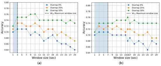
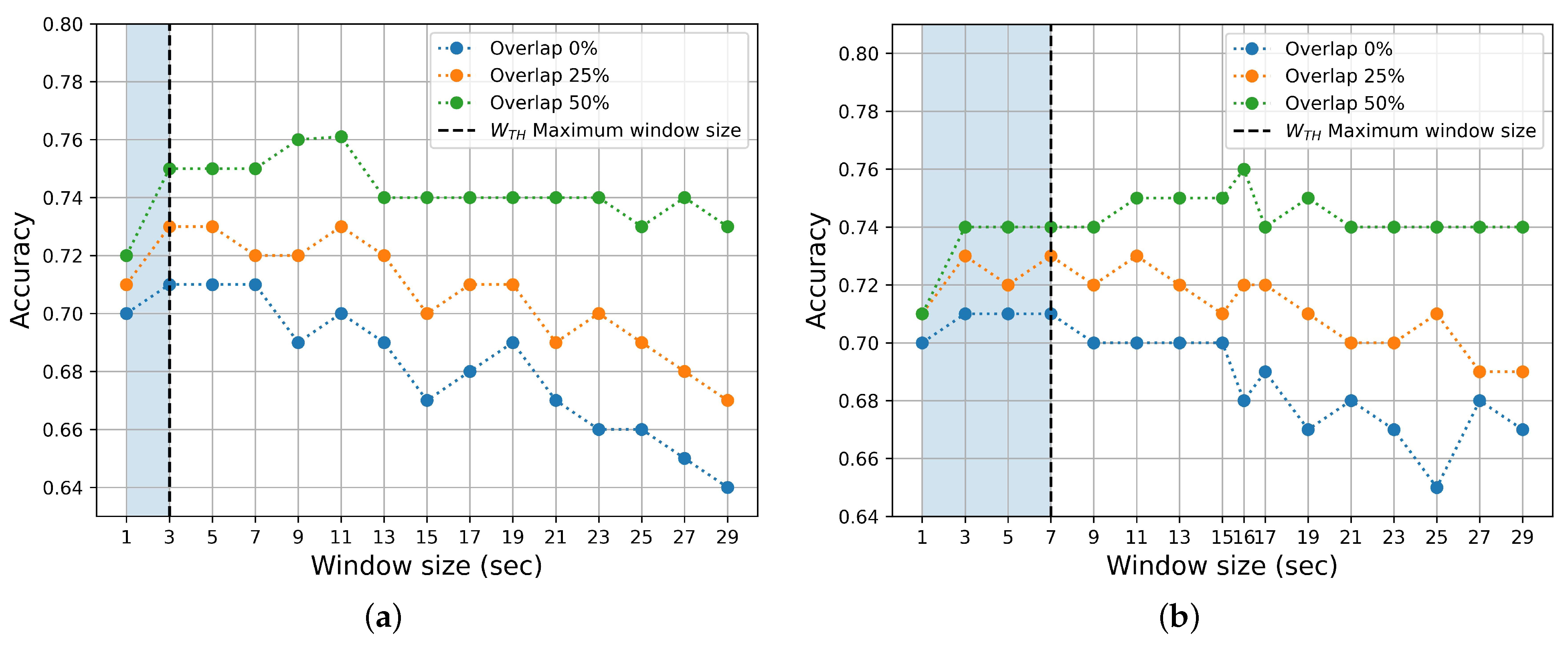
Figure 5.
Mean Accuracy performance for different window duration sizes and percentages of overlap, employing Random Forest (RF). The vertical dotted black lines represent the maximum possible window size associated with a representative median (see Figure 6). (a) Arousal. (b) Valence.
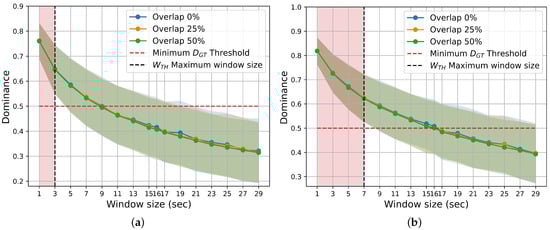
Figure 6.
Mean Dominance ground truth label for different window duration sizes and percentages of overlap. Standard deviations are shown as error bands around the average Dominance, following the color convention of the overlap legend. The vertical dotted black lines represent the maximum possible window size that meets the criterion. (a) Arousal. (b) Valence.
Because we worked with imbalanced data, we added a dummy classifier as a baseline, which makes predictions based on the most frequent class (i.e., always returns the most frequent class in the observed labels). This baseline helps to appreciate the skill of the different tested models.
3.1. Impact of Window Duration Size and Overlap
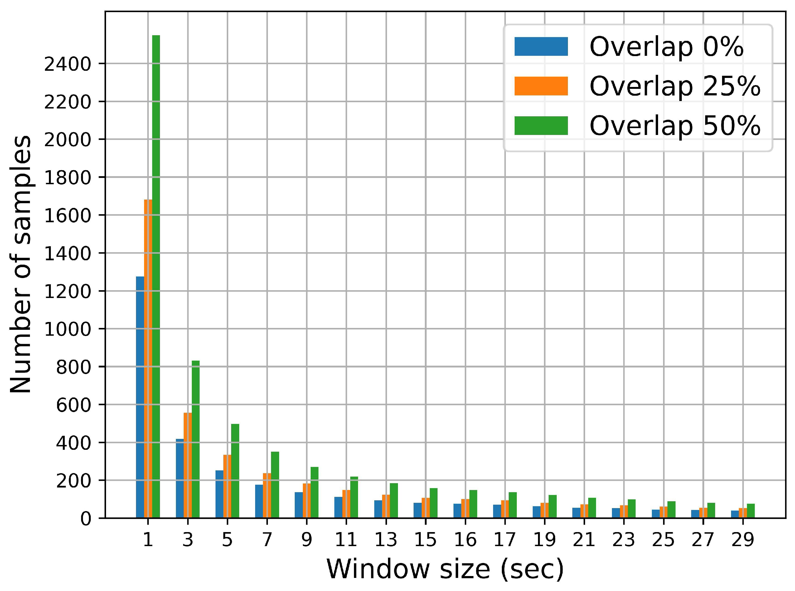
As can be seen in Figure 5, accuracy decreases with increasing window size, both in valence and arousal, when there is no overlap. A similar trend is observed in the accuracy when the . However, when the overlap is , accuracy decreases more slowly. It can be shown that accuracy decreases for window duration sizes greater than 30 s. As expected, the number of window instances also decreases with increasing , as can be seen in Figure 7. For , the optimum window duration size is 3 s for both arousal and valence in terms of ACC, UAR, and F1 scores. Moreover, from our results, all metric scores increase as the overlap increases.
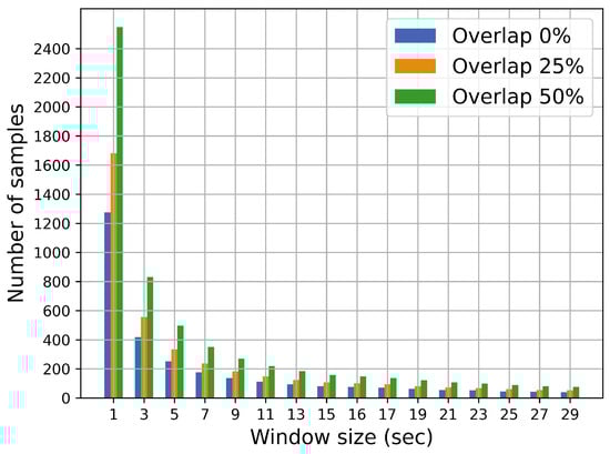
Figure 7.
Number of window instances for different window sizes and percentages of overlap.
3.2. Features Domain Performance Comparison
Both temporal–statistical and nonlinear features were extracted for different window duration sizes and percentages of overlap. In every case, nonlinear features outperformed temporal–statistical features in terms of performance. Figure 8 illustrates this comparison. In the best case, nonlinear features yielded an accuracy of 0.75, while temporal–statistical features achieved 0.69.
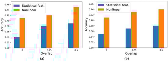
Figure 8.
Features domain performance comparison for optimum window size (), employing Random Forest. (a) Arousal. (b) Valence.
3.3. Labeling Schemes Comparison
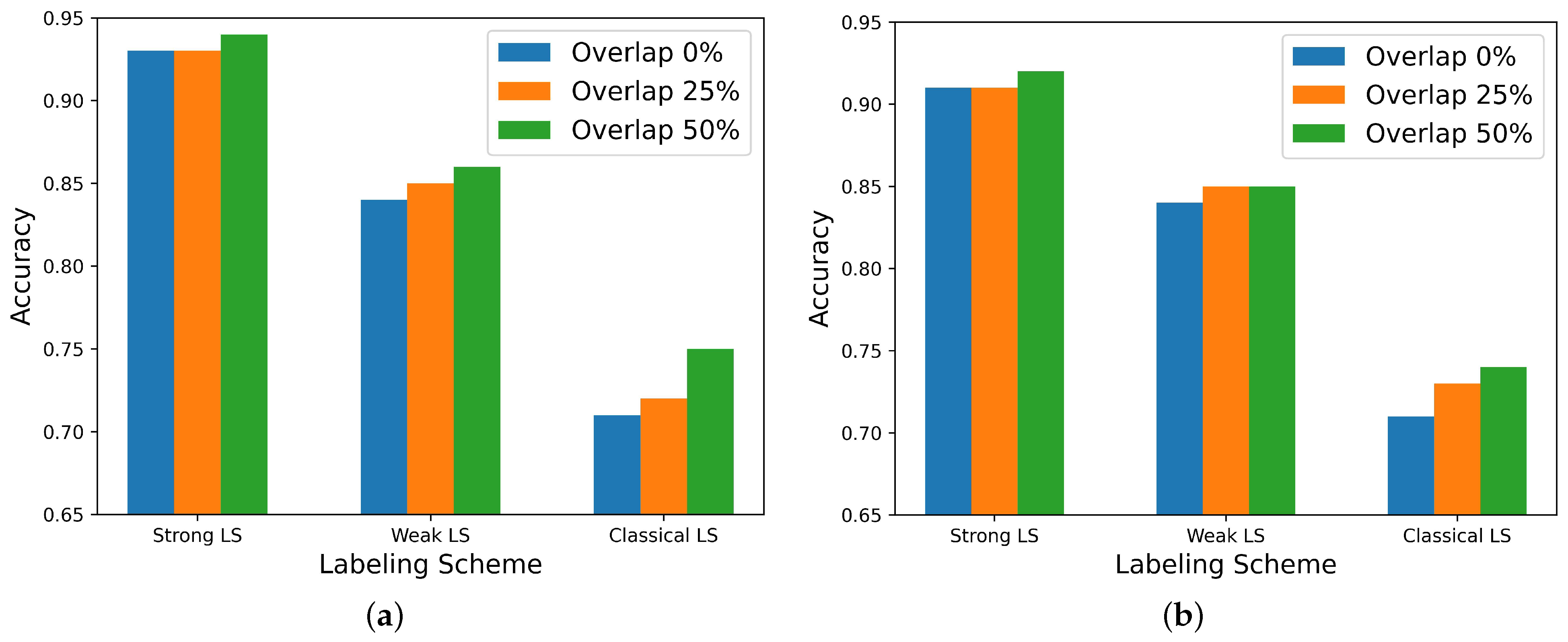
The Strong Labeling Scheme (SLS) proved to be more accurate than the Weak Labeling Scheme (WLS) and the Classic Labeling Scheme (CLS). The best accuracy of 0.92 for valence and 0.94 for arousal was obtained employing the SLS and , as can be seen in Figure 9.
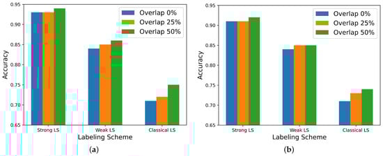
Figure 9.
Labeling scheme performance comparison for optimum window size (), employing Random Forest. (a) Arousal. (b) Valence.
4. Discussion
The main finding is the identification of the optimal window duration for arousal and valence, which is 3 s, for the CASE dataset, using a overlap. It is worth mentioning that these optimal values arise from the fusion of PPG and GSR.
As the overlap increases, four different effects can be identified: (a) accuracy improves, (b) the optimal window duration value rises, (c) an approximate plateau appears for window durations greater than the optimum in the overlap situation, and (d) performance decreases slowly over longer window durations (the curve flattens). It is important to note that accuracy decreases as the window duration grows when there is no overlap, consistent with other studies [18,24]. However, for large values of (i.e., ), the median is not representative (see Figure 6).
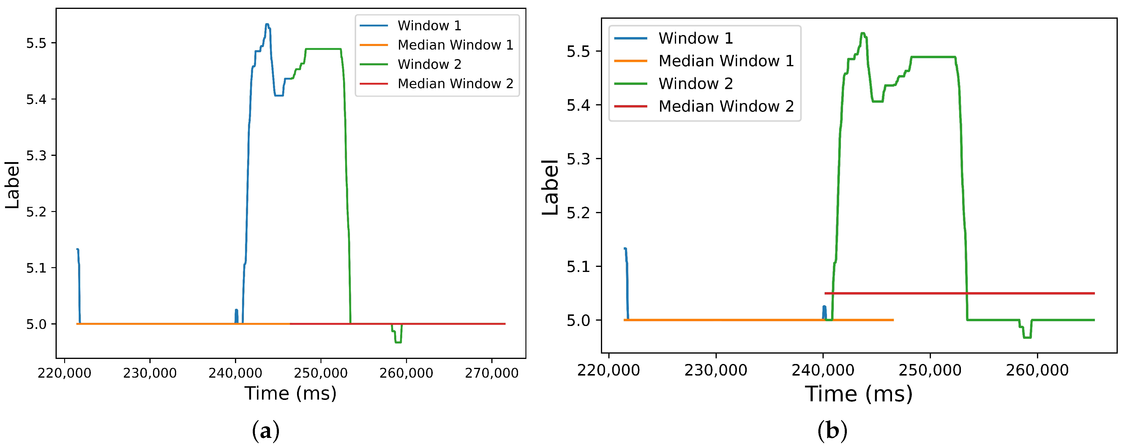
These effects could be due to the reinforcement in the model’s training caused by the overlap, which allows capturing emotional information that would otherwise be missed in the no-overlap situation with the same window duration. The mentioned classification algorithms require a single label value per window (i.e., per instance), which has a ‘filtering’ effect on local label fluctuations in specific parts of the window when the annotations are continuous. However, these local fluctuations can be captured by an adjacent overlapping window, provided that a proper window size and overlap stride are chosen. In this way, the overlap ‘reinforces’ the learning. Without overlap, these local label variations might be ‘missed’ or filtered out, resulting in the loss of emotional information. In Figure 10a, we show two adjacent windows without overlap. Label fluctuations in the last 5 s of the first window are not captured by the median label. However, these fluctuations can be captured by the median of the adjacent window if the overlap is increased, as illustrated in Figure 10b. Interestingly, accuracy does not fall abruptly as window durations increase (see Figure 5). This could be attributed both to the greater volume of data (i.e., a greater number of available data segments comes with increased overlap ratios) and to the reinforcement in learning provided by the overlap.
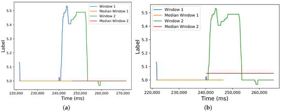
Figure 10.
Median label of two adjacent windows for different overlap situations (window size s). (a) Overlap ; (b) .
Within the range of windows where dominance is acceptable (i.e., ), there appears to be no correlation between the increase in accuracy performance and the decrease in dominance (see Figure 5 and Figure 6). Accuracy increases with greater and . This might be due to the better capture of affective information with a larger window size as well as reinforcement in learning due to the increased overlap.
For s, the number of window instances decreases significantly (see Figure 7). In this situation, the training and testing processes may be less reliable, leading to a reduced generalizability of the model.
Concerning the duration of emotions, studies on the effects of emotions on autonomic nervous system activity typically cover periods ranging from 0.5 to 300 s [7]. Modern datasets using videos as the eliciting stimulus have employed validated videos with durations of 50 to 180 s [14,33]. Although the duration of emotions is highly variable and can range from a few seconds to hours (depending on factors such as the subject, the emotion-eliciting situation, the intensity of the emotion at onset, and the format of the response scale [34,35,36]), it is established in the literature that Event-Related Skin Conductance Responses (ER-SCR) typically take between 2 and 6 s to reach their peak following stimulus onset [37]. Additionally, SCR recovery times (i.e., the duration from peak to full recovery) can vary, resulting in a total SCR duration ranging from 6 to 20 s [38]. However, we were unable to find studies measuring the time response from stimulus onset to significant changes in the PPG waveform. Despite the lack of specific data on PPG response times, the typical durations observed in SCR may be related to the optimal window duration results obtained in this study. Finally, the change in emotion during data collection can be the main reason large window sizes are not good. In this sense, the results shown in Figure 5 may be the longest window sizes available for obtaining the best classification performance.
In summary, smaller window sizes provide a greater number of window instances, which in turn favor training and testing but may not contain sufficient emotional information. Conversely, larger window sizes may capture enough affective data but cannot effectively capture class transitions. A balance between the number of window segments and sufficient emotional content within the window is needed. An optimal window size can provide this balance.
Ayata et al. [18] reported maximum accuracy for one-second overlapped windows of s and s, respectively, using only GSR or PPG. They extracted temporal and statistical features to train the models. The optimal window duration held for both valence and arousal.
On the other hand, Zhang et al. [24] achieved maximum accuracy for a non-overlapped window of s using ECG, PPG, GSR, and Heart Rate (HR) on the CASE dataset for both valence and arousal. For the MERCA dataset, non-overlapped windows of s and s achieved maximum accuracy for arousal and valence, respectively.
The difference in our results might be due to the fusion of PPG and GSR features, the use of nonlinear features, and the continuous annotations binarized using the median method. This suggests that the optimal window duration depends on the biosignals and the particular processing pipeline employed to train the models (i.e., preprocessing method, set of extracted features, continuous vs. discrete annotations, and label mapping method), but especially on the percentage of overlap. To the best of our knowledge, no previous work has studied the reinforcement effect of overlapping windows on continuous annotation datasets using only GSR and PPG biosignals. Further research should be conducted on similar datasets to confirm our findings.
Regarding extracted features, nonlinear outperformed temporal–statistical features in every situation, suggesting a greater skill in extracting emotional information from the biosignals. This is consistent with current trends in nonlinear feature extraction [1,16].
Although [16] showed better accuracy scores using nonlinear feature fusion for GSR and PPG, and a PNN as the classifier, we found that shallow learning algorithms offer a good compromise between performance and low computational cost.
Concerning the labeling scheme, SLS and WLS performed better than CLS, which is as expected because CLS only kept extreme values of the labels while discarding values around the neutral. This facilitated pattern recognition and model training but came at the expense of discarding samples.
Finally, we achieved better results than in our previous work [22], although we applied the same algorithms configured with the same hyperparameter configuration. This suggests that genuine windowing performed on a continuous annotations dataset, combined with the extraction of nonlinear features, proved to extract more emotional information from the biosignals than using a discrete annotation dataset with temporal–statistical features. A comparison with related studies can be seen in Table 6.
Table 6.
Comparison with other other related studies.
4.1. Recommendations for Determining Optimal Window Sizes
We recommend the following steps to identify the optimal window sizes:
- First, determine the range of window sizes where the dominance meets the minimum GT label threshold criterion: . Other window ranges should be excluded from the analysis because non-dominant labels could confuse the classifier.
- Second, identify the best accuracy performance in terms of and within the range of window sizes found in the first step. If only one value meets these requirements, then the optimum combination of and has been found.
- Third, if more than one combination of and has the maximum accuracy within , select the one with higher dominance and the highest number of window instances (i.e., typically occurring with smaller and larger ). This ensures a more representative median label and makes training and testing more reliable. Additionally, it benefits from the reinforcement effect caused by overlapping windows.
- Fourth, careful consideration should be given to the correlation between dominance and accuracy over . For example, a low correlation may better reveal underlying effects that contribute to improved performance. Conversely, a high correlation may make it more difficult to determine whether the increasing accuracy over is due to higher dominance of the label within the window or other factors.
4.2. Limitations
It is worth mentioning that we employed a specific set of algorithm hyperparameters and nonlinear features on a particular dataset. Other combinations should be tested on several continuous annotation datasets to determine which combination exhibits better generalization skills. Additionally, different processing pipelines might yield varying optimum window durations, as the optimal value can depend on the overall processing method.
Some nonlinear features are computationally more costly than others (e.g., the Lyapunov Exponent takes longer to compute than Poincare indices and Approximate Entropy). In future work, we plan to explore other nonlinear features to optimize computational efficiency.
We employed the CASE dataset (see Section 1) to test the working hypotheses on a continuous annotation dataset, allowing for genuine window segmentation. Although this dataset uses FDA-approved sensors, some of its instruments (e.g., the ADC module) are not particularly suited for real-life scenarios. We considered two recent datasets, namely, Emognition [33] and G-REx [41], which use PPG and GSR wearable devices; however, their annotation method is not continuous.
Despite the fact that the median method allows for performing a window sensitivity analysis without discarding window instances a priori, it requires computing the dominance GT label and employing the minimum GT label threshold criterion. A standard majority method could be used instead, excluding segments without a clear majority from training and testing. Attention should be paid to the number of samples to ensure the dataset has sufficient instances for both training and testing.
In practice, a sensitivity analysis should be conducted for each individual due to the high variability in emotions, discarding windows where the metric (median or simple majority) is not representative. If too many windows are discarded, additional samples may be needed to increase the data available for training. Although this is not always possible, as more commercial FDA-approved GSR and PPG wearable sensors continue to emerge, the availability of data samples for model training in real-life situations will increase [6,42]. This increased data availability might make continuous annotation unnecessary. In this situation, SLS could be employed when there is interest only in very definite emotions (high or low arousal, high or low valence, no neutral values). Samples discarded by this scheme might be compensated for by a larger data volume, keeping the model training robust.
5. Conclusions
In this work, we performed a genuine window sensitivity study to determine the window duration that optimized emotion recognition accuracy for valence and arousal based only on PPG and GSR. We tested different percentages of overlap in a continuous annotation dataset and found a benefit from the reinforcement effect caused by overlapping windows. Additionally, we compared the performance of nonlinear and temporal–statistical features, verifying that the former extracts more emotional information from the biosignals.
We confirmed that recognizing emotions with acceptable accuracy is possible using only the mentioned biosignals, provided that continuous labeling, nonlinear features, optimized window size, and overlap percentage, along with a minimum GT label threshold criterion, are employed. Under these conditions, well-known shallow learning algorithms offer a good compromise between performance and low computational cost. Furthermore, if the SLS scheme is used, excellent performance can be achieved, although some samples may be discarded. This issue could be mitigated by employing wearables in longitudinal real-life scenarios, given their potential to gather larger volumes of data.
Author Contributions
Conceptualization, M.F.B., V.H. and M.R.; methodology, M.F.B., V.H. and M.R.; software, M.F.B.; validation, M.F.B., V.H. and M.R.; formal analysis, M.F.B.; investigation, M.F.B.; resources, V.H.; data curation, M.F.B.; writing—original draft preparation, M.F.B.; writing—review and editing, M.F.B., V.H. and M.R.; visualization, M.F.B.; supervision, V.H. and M.R.; project administration, V.H.; funding acquisition, V.H. All authors have read and agreed to the published version of the manuscript.
Funding
This research was supported by Universidad Austral.
Data Availability Statement
The dataset used in this work is openly available from GitLab at https://gitlab.com/karan-shr/case_dataset (accessed on 1 August 2024). Follow Section 2.7 instructions to reproduce our simulations.
Conflicts of Interest
The authors declare no conflicts of interest.
References
- Khare, S.K.; Blanes-Vidal, V.; Nadimi, E.S.; Acharya, U.R. Emotion recognition and artificial intelligence: A systematic review (2014–2023) and research recommendations. Inf. Fusion 2023, 102, 102019. [Google Scholar] [CrossRef]
- Dzedzickis, A.; Kaklauskas, A.; Bucinskas, V. Human emotion recognition: Review of sensors and methods. Sensors 2020, 20, 592. [Google Scholar] [CrossRef] [PubMed]
- Bota, P.J.; Wang, C.; Fred, A.L.N.; Placido Da Silva, H. A Review, Current Challenges, and Future Possibilities on Emotion Recognition Using Machine Learning and Physiological Signals. IEEE Access 2019, 7, 140990–141020. [Google Scholar] [CrossRef]
- Schmidt, P.; Reiss, A.; Dürichen, R.; Laerhoven, K.V. Wearable-Based Affect Recognition—A Review. Sensors 2019, 19, 4079. [Google Scholar] [CrossRef] [PubMed]
- Davoli, L.; Martalò, M.; Cilfone, A.; Belli, L.; Ferrari, G.; Presta, R.; Montanari, R.; Mengoni, M.; Giraldi, L.; Amparore, E.G.; et al. On driver behavior recognition for increased safety: A roadmap. Safety 2020, 6, 55. [Google Scholar] [CrossRef]
- Gomes, N.; Pato, M.; Lourenço, A.R.; Datia, N. A Survey on Wearable Sensors for Mental Health Monitoring. Sensors 2023, 23, 1330. [Google Scholar] [CrossRef]
- Kreibig, S.D. Autonomic nervous system activity in emotion: A review. Biol. Psychol. 2010, 84, 394–421. [Google Scholar] [CrossRef]
- van Dooren, M.; de Vries, J.J.J.; Janssen, J.H. Emotional sweating across the body: Comparing 16 different skin conductance measurement locations. Physiol. Behav. 2012, 106, 298–304. [Google Scholar] [CrossRef]
- Rinella, S.; Massimino, S.; Fallica, P.G.; Giacobbe, A.; Donato, N.; Coco, M.; Neri, G.; Parenti, R.; Perciavalle, V.; Conoci, S. Emotion Recognition: Photoplethysmography and Electrocardiography in Comparison. Biosensors 2022, 12, 811. [Google Scholar] [CrossRef] [PubMed]
- Huang, Y.; Yang, J.; Liu, S.; Pan, J. Combining facial expressions and electroencephalography to enhance emotion recognition. Future Internet 2019, 11, 105. [Google Scholar] [CrossRef]
- Koelstra, S.; Mühl, C.; Soleymani, M.; Lee, J.S.; Yazdani, A.; Ebrahimi, T.; Pun, T.; Nijholt, A.; Patras, I. DEAP: A database for emotion analysis; Using physiological signals. IEEE Trans. Affect. Comput. 2012, 3, 18–31. [Google Scholar] [CrossRef]
- Miranda-Correa, J.A.; Abadi, M.K.; Sebe, N.; Patras, I. AMIGOS: A Dataset for Affect, Personality and Mood Research on Individuals and Groups. IEEE Trans. Affect. Comput. 2021, 12, 479–493. [Google Scholar] [CrossRef]
- Park, C.Y.; Cha, N.; Kang, S.; Kim, A.; Khandoker, A.H.; Hadjileontiadis, L.; Oh, A.; Jeong, Y.; Lee, U. K-EmoCon, a multimodal sensor dataset for continuous emotion recognition in naturalistic conversations. Sci. Data 2020, 7, 293. [Google Scholar] [CrossRef] [PubMed]
- Sharma, K.; Castellini, C.; van den Broek, E.L.; Albu-Schaeffer, A.; Schwenker, F. A dataset of continuous affect annotations and physiological signals for emotion analysis. Sci. Data 2019, 6, 196. [Google Scholar] [CrossRef]
- Zitouni, M.S.; Park, C.Y.; Lee, U.; Hadjileontiadis, L.J.; Khandoker, A. LSTM-Modeling of Emotion Recognition Using Peripheral Physiological Signals in Naturalistic Conversations. IEEE J. Biomed. Heal. Inform. 2023, 27, 912–923. [Google Scholar] [CrossRef]
- Goshvarpour, A.; Goshvarpour, A. The potential of photoplethysmogram and galvanic skin response in emotion recognition using nonlinear features. Phys. Eng. Sci. Med. 2020, 43, 119–134. [Google Scholar] [CrossRef]
- Martinez, H.P.; Bengio, Y.; Yannakakis, G. Learning deep physiological models of affect. IEEE Comput. Intell. Mag. 2013, 8, 20–33. [Google Scholar] [CrossRef]
- Ayata, D.; Yaslan, Y.; Kamasak, M.E. Emotion Based Music Recommendation System Using Wearable Physiological Sensors. IEEE Trans. Consum. Electron. 2018, 64, 196–203. [Google Scholar] [CrossRef]
- Kang, D.H.; Kim, D.H. 1D Convolutional Autoencoder-Based PPG and GSR Signals for Real-Time Emotion Classification. IEEE Access 2022, 10, 91332–91345. [Google Scholar] [CrossRef]
- Maeng, J.H.; Kang, D.H.; Kim, D.H. Deep Learning Method for Selecting Effective Models and Feature Groups in Emotion Recognition Using an Asian Multimodal Database. Electronics 2020, 9, 1988. [Google Scholar] [CrossRef]
- Domínguez-Jiménez, J.A.; Campo-Landines, K.C.; Martínez-Santos, J.C.; Delahoz, E.J.; Contreras-Ortiz, S.H. A machine learning model for emotion recognition from physiological signals. Biomed. Signal Process. Control 2020, 55, 101646. [Google Scholar] [CrossRef]
- Bamonte, M.F.; Risk, M.; Herrero, V. Emotion Recognition Based on Galvanic Skin Response and Photoplethysmography Signals Using Artificial Intelligence Algorithms. In Advances in Bioengineering and Clinical Engineering; Ballina, F.E., Armentano, R., Acevedo, R.C., Meschino, G.J., Eds.; Springer: Cham, Switzerland, 2024; pp. 23–35. [Google Scholar] [CrossRef]
- Makowski, D.; Pham, T.; Lau, Z.J.; Brammer, J.C.; Lespinasse, F.; Pham, H.; Schölzel, C.; Chen, S.H. NeuroKit2: A Python toolbox for neurophysiological signal processing. Behav. Res. Methods 2021, 53, 1689–1696. [Google Scholar] [CrossRef]
- Zhang, T.; Ali, A.E.; Wang, C.; Hanjalic, A.; Cesar, P. Corrnet: Fine-grained emotion recognition for video watching using wearable physiological sensors. Sensors 2021, 21, 52. [Google Scholar] [CrossRef]
- Boyer, R.S.; Moore, J.S. MJRTY—A Fast Majority Vote Algorithm. In Automated Reasoning: Essays in Honor of Woody Bledsoe; Boyer, R.S., Ed.; Springer Netherlands: Dordrecht, The Netherlands, 1991; pp. 105–117. [Google Scholar] [CrossRef]
- Menezes, M.L.; Samara, A.; Galway, L.; Sant’Anna, A.; Verikas, A.; Alonso-Fernandez, F.; Wang, H.; Bond, R. Towards emotion recognition for virtual environments: An evaluation of eeg features on benchmark dataset. Pers. Ubiquitous Comput. 2017, 21, 1003–1013. [Google Scholar] [CrossRef]
- Rosenstein, M.T.; Collins, J.J.; De Luca, C.J. A practical method for calculating largest Lyapunov exponents from small data sets. Phys. D Nonlinear Phenom. 1993, 65, 117–134. [Google Scholar] [CrossRef]
- Godin, C.; Prost-Boucle, F.; Campagne, A.; Charbonnier, S.; Bonnet, S.; Vidal, A. Selection of the Most Relevant Physiological Features for Classifying Emotion. In Proceedings of the 2nd International Conference on Physiological Computing Systems PhyCS, Angers, France, 11–13 February 2015; pp. 17–25. [Google Scholar] [CrossRef]
- van Gent, P.; Farah, H.; van Nes, N.; van Arem, B. Analysing noisy driver physiology real-time using off-the-shelf sensors: Heart rate analysis software from the taking the fast lane project. J. Open Res. Softw. 2019, 7, 32. [Google Scholar] [CrossRef]
- Dissanayake, V.; Seneviratne, S.; Rana, R.; Wen, E.; Kaluarachchi, T.; Nanayakkara, S. SigRep: Toward Robust Wearable Emotion Recognition with Contrastive Representation Learning. IEEE Access 2022, 10, 18105–18120. [Google Scholar] [CrossRef]
- Islam, M.R.; Moni, M.A.; Islam, M.M.; Rashed-Al-Mahfuz, M.; Islam, M.S.; Hasan, M.K.; Hossain, M.S.; Ahmad, M.; Uddin, S.; Azad, A.; et al. Emotion Recognition from EEG Signal Focusing on Deep Learning and Shallow Learning Techniques. IEEE Access 2021, 9, 94601–94624. [Google Scholar] [CrossRef]
- Schuller, B.; Vlasenko, B.; Eyben, F.; Wöllmer, M.; Stuhlsatz, A.; Wendemuth, A.; Rigoll, G. Cross-Corpus acoustic emotion recognition: Variances and strategies. IEEE Trans. Affect. Comput. 2010, 1, 119–131. [Google Scholar] [CrossRef]
- Saganowski, S.; Komoszyńska, J.; Behnke, M.; Perz, B.; Kunc, D.; Klich, B.; Kaczmarek, Ł.D.; Kazienko, P. Emognition dataset: Emotion recognition with self-reports, facial expressions, and physiology using wearables. Sci. Data 2022, 9, 158. [Google Scholar] [CrossRef]
- Verduyn, P.; Delvaux, E.; Van Coillie, H.; Tuerlinckx, F.; Mechelen, I.V. Predicting the Duration of Emotional Experience: Two Experience Sampling Studies. Emotion 2009, 9, 83–91. [Google Scholar] [CrossRef]
- Verduyn, P.; Van Mechelen, I.; Tuerlinckx, F. The relation between event processing and the duration of emotional experience. Emotion 2011, 11, 20–28. [Google Scholar] [CrossRef] [PubMed]
- Verduyn, P.; Tuerlinckx, F.; Van Gorp, K. Measuring the duration of emotional experience: The influence of actual duration and response format. Qual. Quant. 2013, 47, 2557–2567. [Google Scholar] [CrossRef]
- Dawson, M.E.; Schell, A.M.; Courtney, C.G. The skin conductance response, anticipation, and decision-making. J. Neurosci. Psychol. Econ. 2011, 4, 111–116. [Google Scholar] [CrossRef]
- Boucsein, W. Electrodermal Activity, 2nd ed.; Springer: New York, NY, USA, 2012. [Google Scholar] [CrossRef]
- Santamaria-Granados, L.; Munoz-Organero, M.; Ramirez-Gonzalez, G.; Abdulhay, E.; Arunkumar, N. Using Deep Convolutional Neural Network for Emotion Detection on a Physiological Signals Dataset (AMIGOS). IEEE Access 2019, 7, 57–67. [Google Scholar] [CrossRef]
- Cittadini, R.; Tamantini, C.; Scotto di Luzio, F.; Lauretti, C.; Zollo, L.; Cordella, F. Affective state estimation based on Russell’s model and physiological measurements. Sci. Rep. 2023, 13, 9786. [Google Scholar] [CrossRef]
- Bota, P.; Brito, J.; Fred, A.; Cesar, P.; Silva, H. A real-world dataset of group emotion experiences based on physiological data. Sci. Data 2024, 11, 116. [Google Scholar] [CrossRef]
- Bustos-López, M.; Cruz-Ramírez, N.; Guerra-Hernández, A.; Sánchez-Morales, L.N.; Cruz-Ramos, N.A.; Alor-Hernández, G. Wearables for Engagement Detection in Learning Environments: A Review. Biosensors 2022, 12, 509. [Google Scholar] [CrossRef]

Disclaimer/Publisher’s Note: The statements, opinions and data contained in all publications are solely those of the individual author(s) and contributor(s) and not of MDPI and/or the editor(s). MDPI and/or the editor(s) disclaim responsibility for any injury to people or property resulting from any ideas, methods, instructions or products referred to in the content. |
© 2024 by the authors. Licensee MDPI, Basel, Switzerland. This article is an open access article distributed under the terms and conditions of the Creative Commons Attribution (CC BY) license (https://creativecommons.org/licenses/by/4.0/).