Article

Research on Energy Management in Hydrogen–Electric Coupled Microgrids Based on Deep Reinforcement Learning

1
College of Automation, Nanjing University of Posts and Telecommunications, Nanjing 210023, China
2
Institute of Advanced Technology for Carbon Neutrality, Nanjing University of Posts and Telecommunications, Nanjing 210023, China
*
Author to whom correspondence should be addressed.
Electronics 2024, 13(17), 3389; https://doi.org/10.3390/electronics13173389
Submission received: 2 August 2024 / Revised: 23 August 2024 / Accepted: 24 August 2024 / Published: 26 August 2024

Abstract

:
Hydrogen energy represents an ideal medium for energy storage. By integrating hydrogen power conversion, utilization, and storage technologies with distributed wind and photovoltaic power generation techniques, it is possible to achieve complementary utilization and synergistic operation of multiple energy sources in the form of microgrids. However, the diverse operational mechanisms, varying capacities, and distinct forms of distributed energy sources within hydrogen-coupled microgrids complicate their operational conditions, making fine-tuned scheduling management and economic operation challenging. In response, this paper proposes an energy management method for hydrogen-coupled microgrids based on the deep deterministic policy gradient (DDPG). This method leverages predictive information on photovoltaic power generation, load power, and other factors to simulate energy management strategies for hydrogen-coupled microgrids using deep neural networks and obtains the optimal strategy through reinforcement learning, ultimately achieving optimized operation of hydrogen-coupled microgrids under complex conditions and uncertainties. The paper includes analysis using typical case studies and compares the optimization effects of the deep deterministic policy gradient and deep Q networks, validating the effectiveness and robustness of the proposed method.

1. Introduction

Hydrogen energy, with its advantages of cleanliness, greenness, high energy density, and ease of storage and transportation, has emerged as a significant form of new energy following wind and photovoltaic power. The development and utilization of hydrogen energy can, on one hand, provide essential raw materials for industries such as chemical manufacturing, pharmaceuticals, and refining through large-scale hydrogen production. On the other hand, hydrogen–electric conversion technologies using fuel cells and electrolytic hydrogen production devices offer stable and reliable resources for regulating power systems. Particularly, in microgrid systems where distributed wind power and photovoltaic power serve as primary energy sources, the integration of hydrogen energy can effectively address issues of power fluctuations and supply reliability during independent microgrid operations.
To explore the feasibility and reliability of hydrogen–electric coupled microgrid systems, scholars both domestically and internationally have conducted in-depth research. Reference [1] provides a comprehensive analysis of the conversion mechanisms and coupling relationships between various energy forms, including solar, hydrogen, and electrical energy. It establishes a digital simulation experimental system for hydrogen–electric coupling that incorporates photovoltaic generation, fuel cells, and electrolytic hydrogen production systems, demonstrating the multi-energy complementarity and coordinated control characteristics of the hydrogen–electric coupling system. Reference [2] investigates the modeling and operational control methods for wind power, photovoltaic systems, hydrogen production, and supercapacitor grid-connected systems, utilizing supercapacitors to quickly smooth out DC voltage fluctuations, thus ensuring the safe and stable operation of hydrogen–electric coupled microgrids in grid-connected states. Reference [3] proposes an optimized dispatch strategy for hydrogen–electric hybrid microgrids based on vehicle-to-grid integration technology, aimed at reducing wind and solar energy wastage, increasing system benefits, and enhancing the reliability of energy supply. Reference [4] addresses the problem of large-scale wind and solar energy curtailment and grid connection issues for wind–solar–hydrogen storage microgrid systems by employing hydrogen storage technology and particle swarm optimization algorithms to achieve economical and stable system operation. Reference [5] coordinates different energy devices in hydrogen–electric coupled microgrids through the establishment of a mixed-integer linear programming (MILP) model. Reference [6] considers the uncertainties in intermittent renewable energy generation and energy demand, deriving optimal energy management strategies for component subsystems based on a two-stage stochastic optimization framework. These references provide strong support for the feasibility and reliability of hydrogen–electric coupled microgrids; however, they still face limitations due to reliance on precise modeling for overall optimization in energy management and scheduling. In contrast, in model-free reinforcement learning methods, agents learn how to make decisions by processing data from their interactions with the environment, without needing predefined knowledge of the environment’s internal mechanisms, offering new perspectives for energy management in hydrogen–electric coupled microgrids.
The literature [7] describes the energy management scheme of deep reinforcement learning in a single building energy subsystem, multiple energy subsystems of a building, and a building microgrid; the literature [8] applies the Q-learning algorithm to propose a low-carbon operation method for an integrated regional energy system, and the study shows that the method can take advantage of the multi-energy complementarity of the integrated energy system and improve its economy. The literature [9] constructs a subsidy price decision optimization model based on the Markov Decision Process (MDP) framework with the objective of maximizing the combined revenue of electricity sellers and users, and the results analyze the effectiveness of the improved model. The literature [10], based on the battery state, charging and discharging actions, electricity price, and other factors, shows that the operational efficiency of hydrogen-power coupled microgrid energy storage is effectively enhanced by an improved deep Q network algorithm with a sequential sample priority adaptive adjustment strategy. The literature [11] applies Q-learning to solve the dynamic pricing optimization problem of microgrids, but the Q-table used in Q-learning is prone to dimensional catastrophe problems with the growth of the size of the problem under study. The literature [12] proposes a deep reinforcement learning-based energy optimization and a management method for hydrogen power coupled microgrids for the conversion use and joint optimal operation of hydrogen, wind, and solar energy forms for smart grid demand side information uncertainty. The literature [13] uses deep Q networks to learn environmental information, such as predicted loads, renewable energy power outputs, such as wind/light, and time-of-day tariffs, and then performs energy management for microgrids through the learned set of strategies. The literature [14] modeled microgrid energy management (MDP) with the objective of minimizing the daily operation cost. A deep feedforward neural network was designed to approximate the optimal action value function, and a DQN algorithm was used to train the neural network. However, in hydrogen–electric coupled microgrids, the decision-making actions of individual energy storage devices are continuous, and the use of a deep Q network algorithm greatly increases the difficulty of convergence and the computational complexity, making policy-based reinforcement learning algorithms more appropriate in this scenario.
Given these limitations, researchers have begun to explore the application of policy-based DRL methods to solve energy management problems with continuous action spaces [15,16]. These methods utilize dnn to directly output deterministic action values or probabilities of executing an action, thus effectively handling continuous action problems and enabling finer-grained energy management [17]. The literature [18] devised an appliance scheduling methodology applying trust region policy optimization (TRPO) for participating in demand response schemes with real-time tariffs. However, calculating the conjugate gradient makes the computational process of the method very complex. In order to improve the computational efficiency of the model, a real-time energy management method for microgrids based on proximal policy optimization (PPO) has been proposed in the literature [19]. However, the on-policy approach has the same goal and action strategies, which limits the exploration capability of the intelligent body and leads it to learn sub-optimal action strategies. Ref. [20] proposed a microgrid scheduling method based on the deep deterministic policy gradient (DDPG). This method minimizes power costs and ensures safe operation of the microgrid.
The above studies provide a reliable basis for the application of the DDPG algorithm to microgrid energy management, but none of them proposes an effective energy management strategy for microgrids involving hydrogen energy. In this paper, we propose an intelligent method based on the deep deterministic strategy gradient for the energy management problem of hydrogen–electric coupled microgrids under high uncertainty conditions. The method can take into account uncertainty elements, such as market price signals, charging/hydrogen loads, and photovoltaic (PV) power variations, with the goal of maximizing the comprehensive operational benefits of hydrogen–electric coupled microgrids during the decision cycle, autonomously predicting the operational scenarios of microgrids through deep and reinforcement learning, and making optimal decisions. As a whole, the main contributions of this paper are as follows:
  • Intelligent hydrogen–electric coupled microgrid energy management strategy: This paper proposes an energy management strategy based on the DDPG. A deep neural network is used to simulate and optimize the energy management strategy of the microgrid by combining the forecast data of PV generation and load demand. The strategy can effectively cope with the influence of uncertain factors, such as PV generation, EV charging loads, and hydrogen charging loads on the optimization results, and ensure that the system supply and demand are balanced throughout the dispatch cycle.
  • Optimization of system operation economics and the reduction in light shedding: The DDPG algorithm operates hydrogen production from excess power during peak PV generation hours, which achieves full utilization of PV power and reduces light shedding. In addition, the method achieves a reduction in the system power purchase cost and improves the overall economic efficiency through the operation of charging and hydrogen production during low-price hours and discharging and selling power during high-price hours.
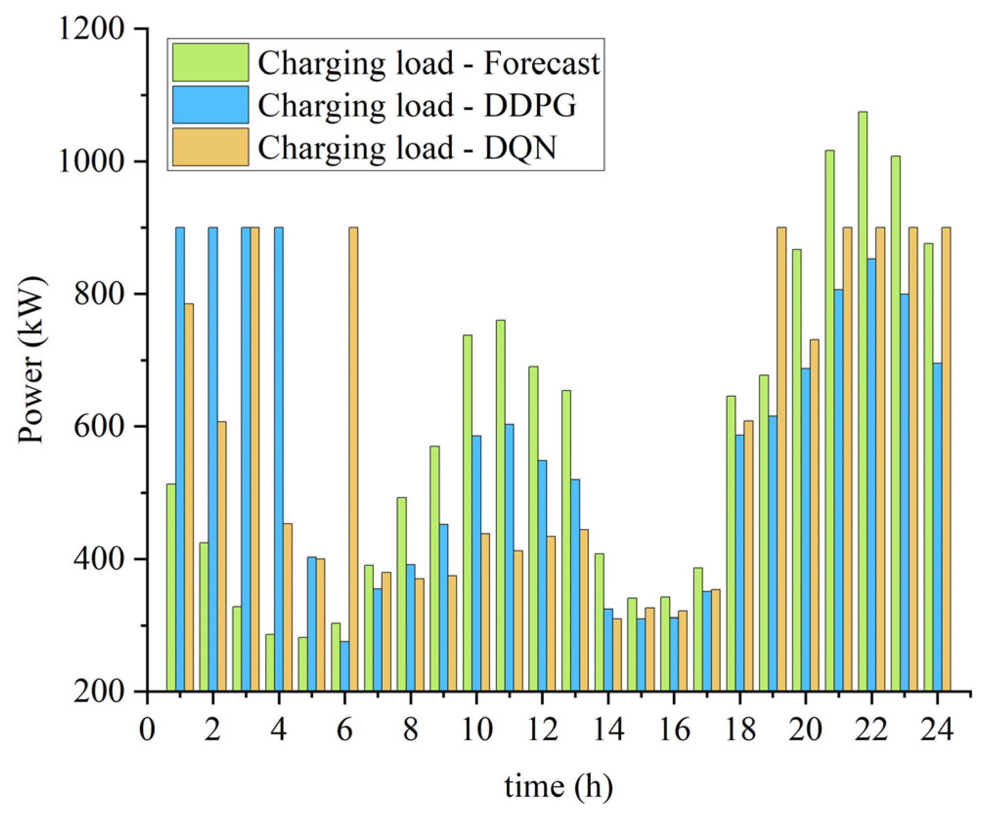
  • Load smoothing and grid stability enhancement: Through the optimal scheduling of EV charging loads, the time and magnitude of peak loads are reduced, and the optimized charging load curves are smoother, which significantly reduces the gap between the peaks and valleys of the grid loads and thus enhances the stability and operational efficiency of the grid.
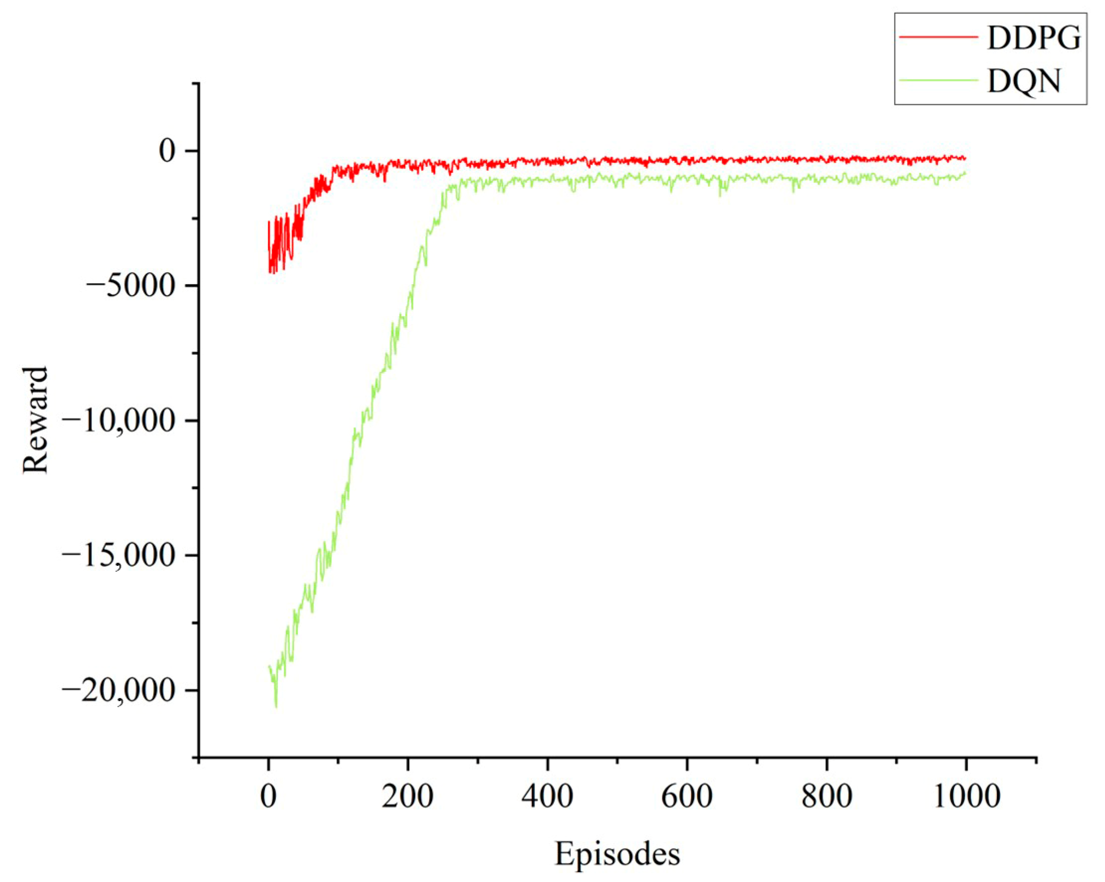
  • The effectiveness and superiority of the DDPG algorithm are verified: The accuracy and effectiveness of the DDPG algorithm over the traditional DQN in dealing with continuous action decision-making problems are verified through case studies. The DDPG algorithm is more capable of optimizing the energy management of the microgrid under complex constraints, which significantly reduces the operating cost of the microgrid.

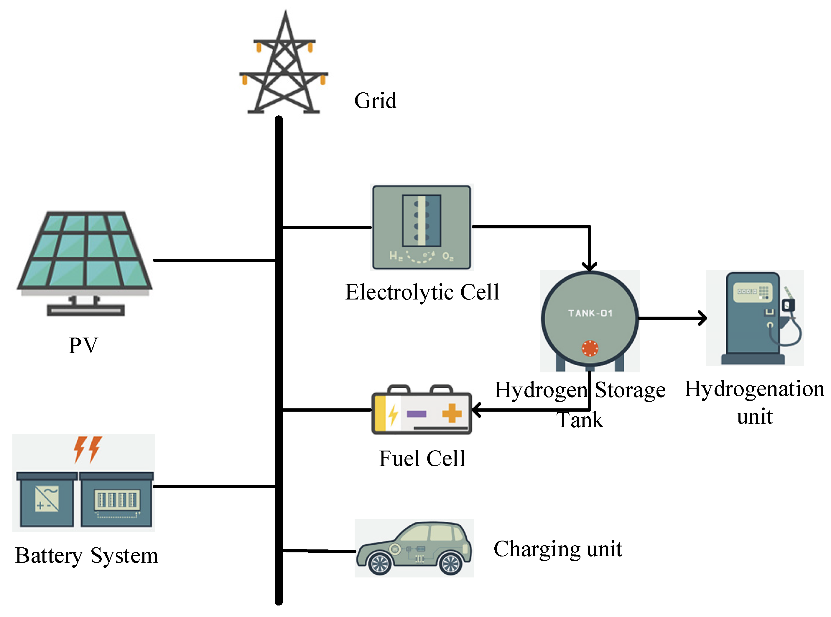
2. Hydrogen–Electric Coupled Microgrid Structure

The hydrogen–electric coupling microgrid studied in this paper consists of photovoltaic generation units, battery systems, electrolytic cells, hydrogen storage tanks, and fuel cells, as well as charging and hydrogenation units. The system architecture is illustrated in Figure 1.
The microgrid utilizes photovoltaic generation facilities and the public grid as its primary energy sources. During system operation, when real-time electricity prices are low or there is an excess of system supply, the energy storage batteries and electrolytic hydrogen production systems are activated, storing surplus electricity or converting it into hydrogen energy. This strategy aims to effectively utilize electricity during periods of low prices and, when real-time prices are high, to meet load demands through the release of stored electricity and hydrogen, thereby optimizing economic benefits. Additionally, the system, in addition to meeting its own needs, can sell excess electricity back to the grid, reducing the occurrence of photovoltaic power waste and promoting the grid integration of photovoltaic power, thereby enhancing the efficiency of renewable energy utilization. This comprehensive energy management strategy not only improves the economic efficiency and operational flexibility of the microgrid but also holds significant importance for achieving efficient energy use and environmental protection.

3. Distributed Energy System Models

3.1. Photovoltaic Power Generation Model

The power output characteristics of photovoltaic generation are influenced by environmental temperature and irradiance and can be approximated using engineering formulas as follows:
P P V = h S T C Q P V G T [ 1 + θ ( T c T r ) ] / G S T C
In the formula, P P V represents the output power of the photovoltaic system; h S T C denotes the power derating factor; Q P V signifies the capacity of the photovoltaic system; G T stands for the irradiance level; θ is the temperature coefficient, with a value of −0.47%/K; T c indicates the operating temperature of the photovoltaic cells; T r is the reference temperature of the cells, typically set at 25 °C; and G S T C refers to the irradiance under standard test conditions.

3.2. Battery Energy Storage System Model

The energy storage batteries play a crucial role in the dynamic regulation of hydrogen–electric coupled microgrid systems, with their charge and discharge models described as follows:
E S O C ( t + 1 ) = E S O C ( t ) P S O C ( t ) × β S O C
β S O C = 0.898 0.173 P S O C ( t ) / P e S O C
In the formula, E S O C ( t ) represents the state of charge of the energy storage battery at a given moment; P S O C ( t ) denotes the operating power of the energy storage battery at that moment, where discharging is positive and charging is negative; β S O C signifies the efficiency of charging or discharging for the energy storage battery; and P e S O C indicates the rated output power of the energy storage battery.

3.3. Electrolytic Hydrogen Production Model

Water electrolysis for hydrogen production can be categorized based on the type of electrolyte used, including alkaline electrolysis, proton exchange membrane (PEM) electrolysis, and solid oxide electrolysis. Among these, proton exchange membrane electrolysis exhibits higher current density, overall efficiency, and hydrogen purity, and also demonstrates a faster dynamic response. The efficiency of hydrogen production using PEM technology is determined by the performance parameters of the electrolysis equipment and the input and output electrical power, with the energy model as follows:
f P H 2 ( t ) P H 2 , max = a P H 2 ( t ) P H 2 , max 2 + b P H 2 ( t ) P H 2 , max + c
V H 2 ( t ) = f ( P H 2 ( t ) P H 2 , max ) π max
In the formula, P H 2 , max represents the rated power of the hydrogen production device; P H 2 ( t ) represents the active power of the hydrogen production device during the period; f P H 2 ( t ) P H 2 , max represents the efficiency coefficient of the hydrogen production device; a , b , c represents the coefficient related to the efficiency of the hydrogen production device; V H 2 ( t ) represents the amount of hydrogen produced by the device during the period; and π max denotes the rated capacity of the hydrogen production module.

3.4. Hydrogen Fuel Cell Model

Hydrogen fuel cells achieve energy management and balance in hydrogen–electric coupled microgrids through efficient energy storage and clean power generation, thereby enhancing system reliability and flexibility and promoting the integration of renewable energy sources. The calculation of their output power is depicted in Equation (6) as follows:
P F C ( t ) = η t V t H n g
In the equation, P F C ( t ) denotes the electric power output of the hydrogen fuel cell at time t , V t represents the rate of hydrogen gas consumption, H n g signifies the heating value of hydrogen, and η t denotes the energy conversion efficiency of the hydrogen fuel cell.

3.5. Model of Hydrogen Storage Facilities

The energy storage facility of the hydrogen–electric coupled microgrid is a hydrogen storage system, characterized by the following energy storage and release attributes:
E H 2 ( t + 1 ) = E H 2 ( t ) + η H 2 V H 2 ( t ) η H V V H V ( t )
In the formula, E H 2 ( t ) denotes the remaining energy of the hydrogen storage system at the end of the t period; η H 2 represents the hydrogen transfer efficiency between the electrolyzer and the storage tank; η H V indicates the hydrogen transfer efficiency between the storage tank and the refueling station; and V H V ( t ) signifies the refueling rate of the refueling station during the t period.

4. Decision-Making Model for Microgrid Energy Management

4.1. Objective Function

The energy management of hydrogen–electric coupled microgrids aims to coordinate the outputs of various system components in order to minimize the energy costs of hydrogen–electric coupled microgrids while adhering to technical constraints. The system must integrate considerations of costs arising from grid transactions and operational maintenance, as well as calculate the revenues from charging electric vehicles, refueling hydrogen fuel cell vehicles, and participating in carbon trading and electricity markets. Therefore, the objective function should encompass grid transaction costs, operational maintenance costs, charging revenues, refueling revenues, and carbon reduction benefits, as illustrated in Equation (8).
min f = t = 1 T [ C g r i d ( t ) C E V ( t ) C H V ( t ) ] + C R + C C O 2 = t = 1 T [ P g r i d ( t ) c g r i d ( t ) P E V ( t ) c E V ( t ) P H V ( t ) c H V ( t ) ] · Δ t + C R + C C O 2
In the equation, T represents the total number of time periods corresponding to the time cycle; C g r i d ( t ) denotes the purchasing cost of electricity for the hydrogen–electric coupled microgrid during period t ; C E V ( t ) signifies the charging revenue of the hydrogen–electric coupled microgrid in period t ; C H V ( t ) refers to the hydrogen charging revenue for the hydrogen–electric coupled multi-microgrid system during period t ; P g r i d ( t ) and c g r i d ( t ) indicate the purchasing power and purchasing price of electricity for the hydrogen–electric coupled microgrid in period t ; P E V ( t ) and c E V ( t ) represent the charging power and charging price for the hydrogen–electric coupled microgrid in period t ; P H V ( t ) and P H V ( t ) pertain to the hydrogen charging power and hydrogen price for the hydrogen–electric coupled microgrid in period t ; C R denotes the operation and maintenance costs of the system within the cycle; and C C O 2 signifies the carbon reduction benefits of the system during the cycle.

4.2. Constraints

4.2.1. Power and Energy Balance Constraints

t = 1 T [ P g r i d ( t ) + P P V ( t ) + P F C ( t ) ] = t = 1 T [ P E V ( t ) + P H 2 ( t ) + P S O C ( t ) + P E M ( t ) ]
In the equation, P P V ( t ) denotes the photovoltaic power generation of the hydrogen–electric coupled microgrid during time period t ; P H V ( t ) represents the electrolyzer’s hydrogen production power during time period t ; P S O C ( t ) refers to the energy storage system’s charge and discharge power during time period t , with discharging being positive and charging being negative; and P E M ( t ) signifies the station’s electrical load power during time period t .

4.2.2. Constraints on the Operation of Photovoltaic Power Generation Systems

P P V min ( t ) P P V ( t ) P P V max ( t )
In the equation, P P V min ( t ) and P P V max ( t ) are, respectively, the minimum and maximum photovoltaic output power of the hydrogen–electric coupled microgrid during the t period.

4.2.3. Electrolytic Hydrogen Production System Operational Constraints

  • Operational Constraints of Electrolytic Cells
P H V min P H V ( t ) P H V max
In the equation, P H V min and P H V max represent the lower and upper limits of the power consumed by the electrolyzer during its normal operation in the hydrogen coupling microgrid at time t .
2.
Constraints on Fuel Cell Operation
P F C min P F C ( t ) P F C max
In the equation, P F C ( t ) represents the operational power of the fuel cell during the t period in the hydrogen–electric coupled microgrid and P F C min and P F C max denote the lower and upper limits of the power consumption of the fuel cell during normal operation, respectively.
3.
Hydrogen Storage Tank Operational Constraints
E H 2 min E H 2 ( t ) E H 2 max
In the equation, E H 2 ( t ) denotes the quantity of hydrogen in the storage tank of the hydrogen–electric coupled microgrid during time period t and E H 2 max and E H 2 min denote the upper and lower limits of the storage capacity of the hydrogen tank.

4.2.4. Electrochemical Energy Storage Operational Constraints

P S O C min P S O C t P S O C max
E S O C min E S O C ( t ) E S O C max
In the formula, P S O C max and P S O C min denote the upper and lower limits of the charging and discharging power of the energy storage system; E S O C ( t ) represents the state of charge of the hydrogen storage tank within the hydrogen–electric coupling microgrid during time period t ; and E S O C max and E S O C min denote the upper and lower limits of the energy storage system’s state of charge.

4.2.5. Constraints on the Operation of Charging/Hydrogen Cells

  • Charging Load Constraints
P E V ( t ) = P E V 1 ( t ) + P E V 2 ( t )
In the formula, P E V ( t ) represents the initial charging load demand; P E V 1 ( t ) denotes the schedulable charging load demand; and P E V 2 ( t ) signifies the non-schedulable charging load demand.
2.
Constraints on Charging/Hydrogen Stations
0 P e v ( t ) P e v , r a t e
0 V h v ( t ) V h v , r a t e
In the formula, P e v ( t ) denotes the charging power of an individual charging station during time period t , P e v , r a t e represents the rated power of a single charging station, V h v ( t ) signifies the hydrogen refueling rate of an individual hydrogen station during time period t , and V h v , r a t e stands for the rated refueling rate of the hydrogen station.

5. Optimization Algorithms for Deep Reinforcement Learning

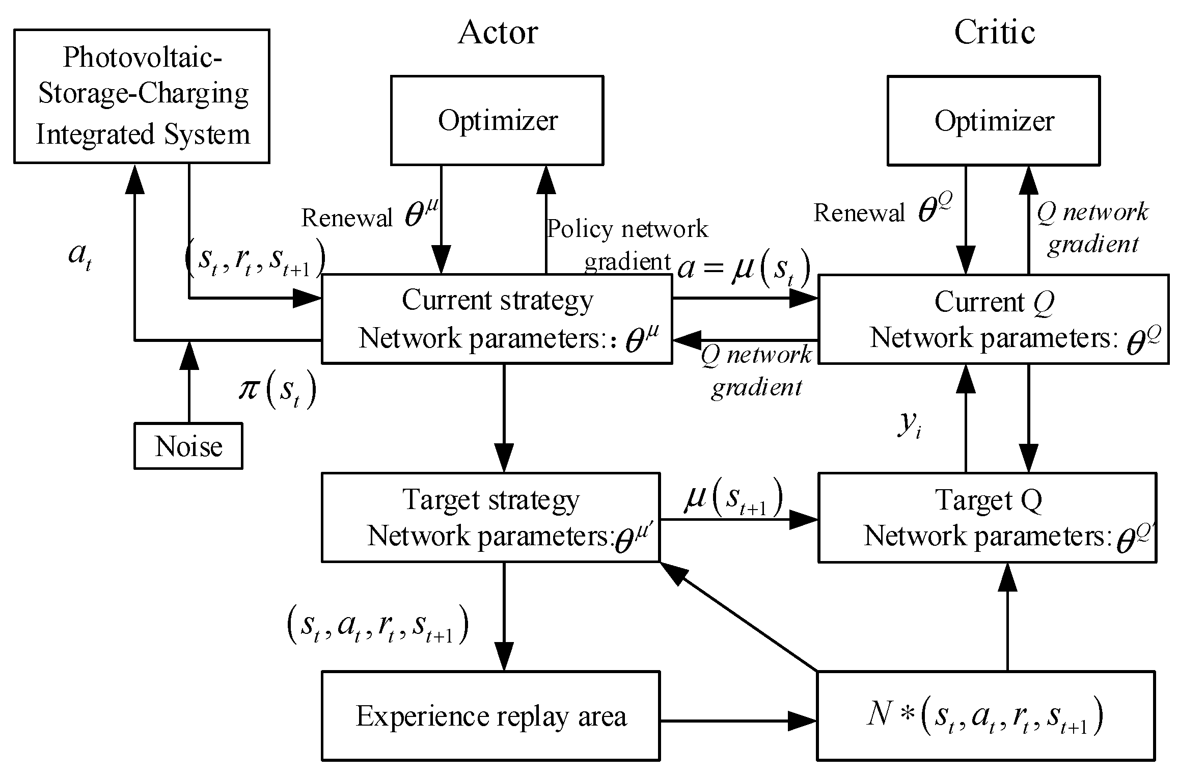
5.1. The Principles of the DDPG Algorithm

Reinforcement learning is fundamentally a sequential decision-making problem, where the agent selects an action based on the currently observable state in order to maximize the accumulated reward. The function that maps states to actions is known as the policy π . Mathematically, this discrete-time interaction process between the agent and the environment is typically described as a Markov Decision Process (MDP).
In reinforcement learning, the agent chooses actions a t from the action space according to the policy π based on the current state s t and receives immediate rewards r t according to the reward function. The accumulated reward R t is defined as the environment’s evaluation of the agent’s actions a t at a given time t .
R t = E k = 0 T γ k r t + k + 1
In the formula, T represents the total number of interactions between the agent and the environment in a learning task, which can be regarded as comprising T periods in this paper; γ is the discount factor that determines the impact of future rewards on the accumulated reward.
The objective of reinforcement learning is to discover the optimal policy π that maximizes the expected cumulative reward of the agent over a period T ; which is
max v π ( s t ) = E π [ R t s t ] = a t π ( a t s t ) s t , r ρ π [ r t + γ v π ( s t + 1 ) ]
In the formula, v π ( s t ) represents the expected cumulative reward of the system at state s t ; s t + 1 denotes the state of the system at the next time step after taking action a t at time t ; and ρ π indicates the probability of transitioning from state s t to state s t + 1 and receiving reward r t after executing action a t according to policy π .
The state-action value function Q ( s t , a t ) denotes the expected long-term return generated under a given policy π and can be expressed as follows:
Q ( s t , a t ) = E a i ~ π [ R t s t , a t ]
The Bellman equation for the state-action value function is expressed as follows:
Q ( s t , a t ) = r t + γ E a t + 1 ~ π [ Q ( s t + 1 , a t + 1 ) ]
The Q-learning algorithm approximates the optimal Q-function through interaction between the agent and the environment, updating iteratively according to Equation (22). Theoretically, under certain conditions, Q-learning can converge to the optimal solution or best outcome as time approaches infinity. However, as engineering problems grow in complexity and the number of states increases, Q-learning becomes increasingly difficult to manage.
The deep Q network (DQN) algorithm integrates deep neural networks with Q-learning. Compared to traditional Q-learning, the DQN stores the Q-value table by approximating the Q-function with a deep neural network. Through interactions between the agent and the environment, the DQN continually refines its action policy, resulting in progressively stabilized cumulative rewards and ultimately achieving reward maximization. Nevertheless, Equation (22) necessitates discretization of the action space, which can lead to excessively large action space dimensions and sub-optimal solutions. Hence, the DQN is less suited for decision-making problems in continuous spaces, such as energy storage discharge and hydrogen tank refilling.
The deep deterministic policy gradient (DDPG) algorithm, based on the actor-critic framework, draws from DQN’s experience replay mechanism and target network concepts, specifically addressing continuous action spaces. The DDPG network comprises both actor and critic networks, including current and target networks. The experience replay mechanism reduces sample correlation by randomly selecting samples from the experience pool during training. The target network maintains fixed parameters over time to eliminate model oscillation caused by identical parameters between the current and target networks. Consequently, the DDPG possesses robust deep neural network fitting and generalization capabilities and excels in continuous action spaces. Furthermore, it can learn the optimal action policy for the current state through ongoing training and adjustment of neural network parameters. Applying this method to energy management in hydrogen–electric coupled microgrids allows for more continuous action outputs and reduced decision-making errors. The structure is as follows The structure is shown in Figure 2.
In the actor-critic framework, the actor network maps the current state to a specific action according to a given policy, as illustrated in Formula (23).
a t = μ s t θ μ + N t
In the formula, μ s t θ μ denotes the function that approximates the state-action mapping relationship, θ μ represents the parameters of the actor network, and N t signifies the noise.
The actor network updates its parameters through policy gradient methods, as illustrated by the following equation:
θ μ J 1 N t a Q s , a θ Q | s = s t , a = μ s t θ μ μ s θ μ | s t
In the formula, Q s , a θ Q denotes the fitting function assessed by the critic network and θ Q represents the parameters of the critic network. The critic network evaluates the action a t chosen under state s t using the formula Q s , a θ Q and updates its parameters by minimizing the loss function. The loss function L is given by the following:
L = 1 N t [ y t Q s t , a t θ Q ] 2
In the equation, y t denotes the target value used for updating the critic network, and can be expressed as follows:
y t = r t + γ Q s t + 1 , μ s t + 1 θ μ θ Q
In the equation, Q s t + 1 , μ s t + 1 θ μ θ Q represents the predicted value function corresponding to the next state s t + 1 . y t can be regarded as the expected return after executing an action a t in the current state s t .
The target network maintains constant parameters over a specific period to eliminate the model oscillation issues arising from the similarity in parameters between the current and target networks. The target network’s update mechanism typically employs the Soft Update method. Soft Update gradually adjusts the target network parameters in each step, causing them to progressively converge towards the main network parameters. The formula for Soft Update is as follows:
θ Q τ θ Q + ( 1 τ ) θ Q
θ μ τ θ μ + ( 1 τ ) θ μ
In the equation, θ Q represents the parameters of the target network for the actor; θ μ denotes the parameters of the target network for the critic; and τ is the coefficient for soft updates.

5.2. Implementation of the DDPG Algorithm

When employing the DDPG algorithm to address the optimization configuration methods and energy management strategies for a hydrogen–electric coupled microgrid, it is essential to design the corresponding state space S, action space A, and reward function R based on the original optimization problem.
  • Definition of the State Space
In the constructed model of the hydrogen–electric coupled microgrid, for any time period t, the state matrix S is constructed to include photovoltaic power generation, non-dispatchable charging load, hydrogen charging load, time-of-use electricity prices, hydrogen storage tank levels, and the charge state of the energy storage system. Thus, the state space of the hydrogen–electric coupled microgrid can be represented as follows:
S = P P V t , P E V 2 t , P H V t , E H 2 ( t ) , E S O C ( t ) , c g r i d ( t ) , c E V ( t ) , c H V ( t )
2.
Definition of the Action Space
In the reinforcement learning process, the agent interacts with the environment, obtaining state information from it and generating an action based on the state matrix. For a hydrogen–electric coupled microgrid, these actions primarily involve power exchanges with the public grid, the charging and discharging power of the battery energy storage system, and the hydrogen production power of the electrolyzer, as well as dispatchable charging loads. Consequently, the action space of the hydrogen–electric coupled microgrid is as follows:
A = P H 2 ( t ) , P S O C ( t ) , P g r i d ( t ) , P E V 1 ( t )
3.
Definition of Reward and Penalty Functions
For the purpose of optimizing the economic operation of hydrogen–electric coupled microgrids, the objectives include minimizing the procurement and sale of electricity costs of the hydrogen–electric coupled microgrid and maximizing the revenue from charging/hydrogen refueling. Let C represent the revenue reward for the hydrogen–electric coupled microgrid, which is defined by the following formula:
C = t = 1 T [ P g r i d ( t ) c g r i d ( t ) P E V ( t ) c E V ( t ) P H V ( t ) c H V ( t ) ] · Δ t
During the iterative process, it is essential to ensure that optimization decisions consistently adhere to the constraints imposed by the regulation of resources. Therefore, incorporating system operational constraints, the penalty function is defined as follows:
D = D p + D S O C + D H 2 = λ d p , t + d S O C , t + d H 2 , t
In the expression, D p represents the penalty for the imbalance of the power system; D S O C represents the penalty for over-discharging or over-charging of the energy storage system; D H 2 represents the penalty for over-discharging or over-charging of the hydrogen storage tank; λ denotes the penalty coefficient; d p , t is the imbalance quantity of the power system at time t ; d S O C , t is the quantity of over-discharging or over-charging of the energy storage system at time t ; and d H 2 , t is the quantity of over-discharging or over-charging of the hydrogen storage tank at time t .
Therefore, the reward function for deep reinforcement learning is defined as follows:
R = C + D
The pseudocode for energy management in a hydrogen–electric coupled microgrid based on the DDPG algorithm is illustrated in Algorithm 1.
Algorithm 1: Energy Management Method for PV-Storage-Charging Integrated System Based on DDPG.
1: Initialize   Actor   network   μ s θ μ   and   Critic   network   Q s , a θ Q
2:Initialize target networks μ and Q , and   set   θ μ θ μ ,   θ Q θ Q
3:Initialize replay buffer D
4:Set soft update coefficient τ and learning rate α
5:for episode =1 to max_episodes do
6:     Initialize random process N for action exploration
7:     Obtain   initial   state   s 1
8:     for  t = 1 to max_steps do
9:            Select   action   a t = μ s t θ μ + N t based on the current policy and exploration
           noise
10:           Execute   action   a t ,   observe   reward   r t   and   next   state   s t + 1
11:           Store   transition   s t , a t , r t , s t + 1 in replay buffer D
12:           Sample   a   random   minibatch   of   s t , a t , r t , s t + 1 from D
13:           Compute   target   y t = r t + γ Q s t + 1 , μ s t + 1 θ μ θ Q
14:           Update   Critic   network   by   minimizing   the   loss   L = 1 N t [ y t Q s t , a t θ Q ] 2
15:           Update Actor network using the sampled policy gradient:
                                                            θ μ J 1 N t a Q s , a θ Q | s = s t , a = μ s t θ μ μ s θ μ | s t
16:           Soft update target networks:
                                                            θ Q τ θ Q + ( 1 τ ) θ Q
                                                            θ μ τ θ μ + ( 1 τ ) θ μ
17:           Update   state   s t s t + 1
18:     end for
19:end for

6. Case Study Analysis

6.1. Case Description

Taking a regional hydrogen–electric coupled microgrid as an example with the parameters shown in Table 1, the system comprises a 600 kW photovoltaic array, an electrical energy storage system with a rated capacity of 360 kW·h, a state of charge ranging from 0.2 to 0.8, a rated power of 100 kW, an electrolyzer with a rated power of 750 kW, where the hydrogen–electric conversion efficiency is estimated at 20%, meaning 5 kWh of electricity can produce 1 Nm3/h of hydrogen, a hydrogen storage tank with a capacity of 1000 Nm3, thirty DC charging stations with a rated power of 30 kW each, providing a total charging capacity of 900 kW, five hydrogen refueling stations with a refueling rate of 30 Nm3/h each, aggregating a total refueling rate of 150 Nm3/h, a hydrogen refueling service price of CNY 5.8/Nm3, and a carbon trading price of CNY 0.07/kg, and the photovoltaic generation and charging/hydrogen load forecast curves for a typical day are illustrated in Figure 3, while the time-of-use electricity pricing is shown in Figure 4.
In Figure 3, it is evident that the predicted electric vehicle charging load peaks at 22:00 with 1188.23 kW and reaches its trough at 14:00 with 251.95 kW, resulting in a peak-to-trough difference of 936.38 kW. Furthermore, during the period from 21:00 to 24:00, the charging load exceeds the maximum power capacity of 900 kW of the DC charging stations. This indicates significant fluctuations in the predicted electric vehicle charging load, with the equipment remaining idle during off-peak periods and potentially operating beyond capacity during peak times, leading to resource wastage and equipment wear.
On the other hand, the hydrogen refueling load during peak periods, such as 22:00, reaches 142.15 Nm3, while during off-peak periods, such as 14:00, it is merely 42.89 Nm3. This demonstrates notable load fluctuations, with a peak-to-trough difference of 99.26 Nm3. The high variability in load increases the complexity of grid management, necessitating frequent adjustments to power generation and storage systems to accommodate load changes, thus escalating operational difficulties and costs. Therefore, it is essential to incentivize users through pricing signals and optimize the system’s energy management strategies through storage systems.

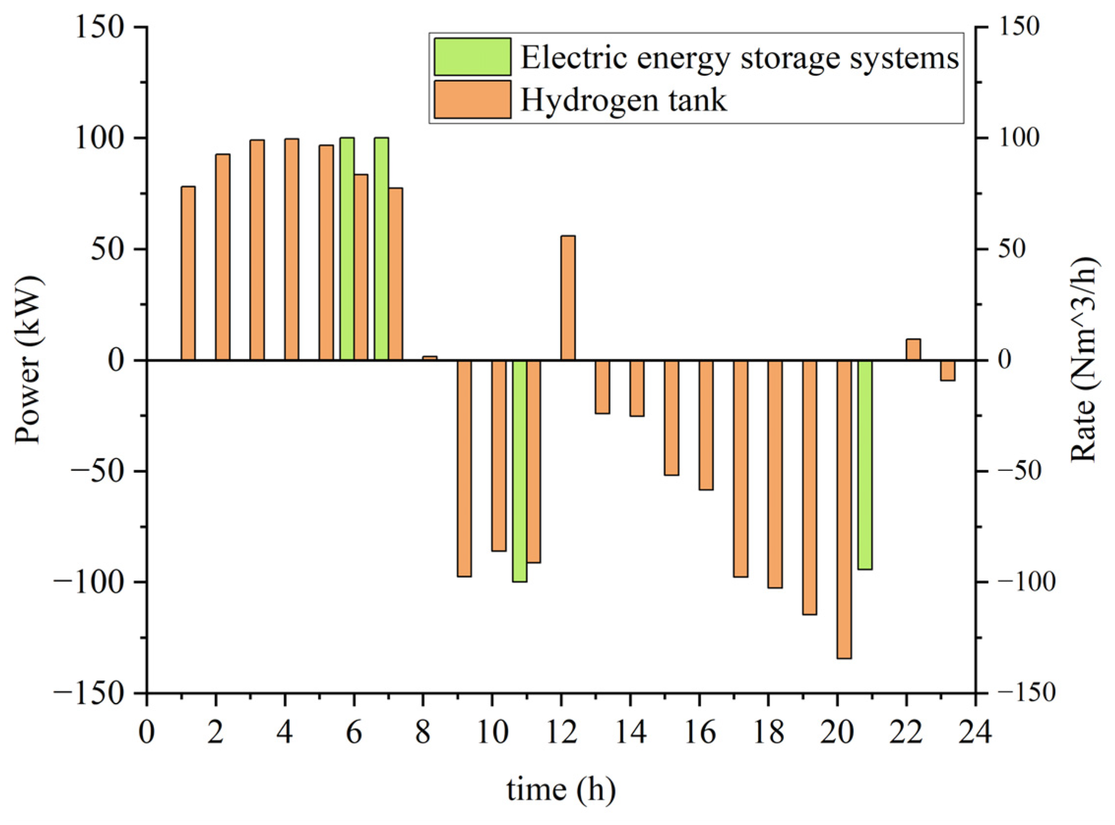
6.2. Simulation Analysis

The DDPG algorithm discussed in this paper is implemented in Python using the PyTorch framework, with the parameter settings detailed in Table 2.
The model training reward curve is illustrated in Figure 5. During the early stages of training with the DDPG algorithm, the model needs to explore the environment, experimenting with various actions and strategies, resulting in a more erratic reward curve. As training progresses, particularly after episodes > 179, the model gradually learns effective strategies and begins making better decisions within the environment. Consequently, the reward curve starts to converge overall, exhibiting only minor, unstable oscillations and approaching stability. Compared to the DQN algorithm, the DDPG algorithm converges more swiftly and achieves a higher reward convergence value, indicating that the energy management strategy under the DDPG algorithm incurs lower costs.
The hydrogen–electric coupled microgrid, through the learned operational strategies for hydrogen storage tanks and electrical energy storage systems (as illustrated in Figure 6), can dynamically adjust the output of these systems based on electricity price signals. During the low-price period from 00:00 to 08:00, the hydrogen storage tanks primarily engage in hydrogen accumulation, achieving a total of 828.11 Nm3, which accounts for 42.45% of the total hydrogen demand, thereby leveraging lower electricity prices to reduce hydrogen production costs. At the photovoltaic power peak period of 13:00, the hydrogen storage tanks use surplus photovoltaic electricity for brief hydrogen accumulation, further diminishing production costs. Additionally, during the low-price period from 07:00 to 09:00, the electrical energy storage system is in charging mode to lower electricity purchase costs, while during the photovoltaic peak period, charging is avoided, ensuring that all excess photovoltaic power is utilized for hydrogen production. By employing the deep deterministic policy gradient (DDPG) algorithm, the microgrid can rationally schedule hydrogen and electricity based on price signals, achieving efficient energy management and cost optimization. This strategy enables hydrogen and battery charging during low-price periods and minimizes energy procurement expenses during high-price periods, thereby optimizing the overall energy cost of the system.
The optimized charging load curve is illustrated in Figure 7, where the demand for unordered charging load amounts to 14,070.96 kWh, with the schedulable charging load totaling 2365.26 kWh. As depicted in Figure 8, unordered charging loads are predominantly concentrated between 10:00 and 14:00 and 19:00 to 23:00. Through energy management optimization, the peak charging load has shifted to between 00:00 and 04:00, redistributing the peak time of electric vehicle charging loads. Moreover, the optimized charging load curve exhibits greater smoothness compared to its predecessor, marked by a reduction in the disparity between peaks and troughs from 936.38 kW to 624.61 kW, a decrease of 33.29%. This not only alleviates pressure on the grid during peak load times but also enhances the utilization rate of the grid during off-peak periods.
Comparing the charging strategies under the DDPG and DQN algorithms as shown in Figure 8, both algorithms achieve the optimization of shifting charging loads to periods of lower electricity prices; however, the charging load curve under the DDPG algorithm is notably smoother. Additionally, Figure 8 reveals that the total hydrogen charging demand is 1950.83 Nm3, with the DDPG algorithm showing an error of 0.01% and the DQN algorithm an error of 4.03%. This indicates that the precision of the DDPG algorithm significantly surpasses that of the DQN algorithm, a benefit stemming from the DDPG’s ability to adjust hydrogen charging quantities within a continuous range (e.g., from 42.89 to 142.15), allowing for finer-grained adjustments, which will be reflected in the operational costs of the microgrid.
Combining the photovoltaic power generation curve shown in Figure 3 with the operational strategy diagram of the hydrogen storage tanks and electric energy storage systems depicted in Figure 6, we analyze the exchange power between the hydrogen–electric coupled microgrid system and the public grid, as illustrated in Figure 9. During the periods from 00:00 to 08:00 and from 21:00 to 24:00, the power purchased from the grid is relatively high, primarily due to substantial electrolyzer operation and electric vehicle charging demands. Conversely, between 11:00 and 16:00, photovoltaic power generation peaks, significantly reducing the need for grid power purchases, and there is even no need to purchase power from the grid between 14:00 and 16:00.
In the aforementioned energy management strategy based on deep reinforcement learning, the total electricity demand for the hydrogen–electric coupling microgrid amounts to 24,476.12 kWh, with a hydrogen consumption of 1950.83 Nm3. The electricity used for hydrogen production is 7805.96 kWh, representing 31.89%; the dispatchable charging load is 14,304.90 kWh, accounting for 58.44%; the controllable charging load is 2365.26 kWh, making up 9.66%; and the system’s conventional electrical load is 819.35 kWh, which constitutes 3.34%. Photovoltaic power generation and the public grid provide electricity for the hydrogen–electric coupling microgrid, with photovoltaic generation totaling 3477.56 kWh, thereby covering 14.21% of the system’s total load demand. The public grid supplies 20,998.56 kWh, representing 85.79% of the total load requirement.
The optimized counterpart is shown in Table 3. In summary, under the DDPG algorithm, the cost of purchasing electricity for the hydrogen coupled microgrid system is CNY 8677.2, the charging revenue is CNY 7838.3, the hydrogen charging revenue is CNY 11,314.79, the carbon revenue is CNY 147.89, the net revenue is CNY 10,623.78, and the pre-optimization net revenue is CNY 9893.74, an increase of CNY 730.04 or an increase of 7.38%. The net revenue of the system under the DQN algorithm is CNY 10,094.95, an increase of CNY 528.8279 or an increase of 5.34%. It can be seen that the energy management strategy proposed in this paper can effectively reduce the operating cost of the hydrogen–electric coupled microgrid.

7. Conclusions

This paper investigates the energy management issues of hydrogen–electric coupled microgrids and proposes an energy management strategy based on the deep deterministic policy gradient (DDPG). This approach utilizes deep neural networks, combined with predictive data on photovoltaic generation and load demands, to simulate and optimize the energy management strategy of the microgrid. The findings indicate that this method can effectively address the impacts of uncertainties such as photovoltaic generation, electric vehicle charging loads, and hydrogen charging loads on the optimization results, ensuring supply–demand balance throughout the entire scheduling cycle. The specific conclusions are as follows:
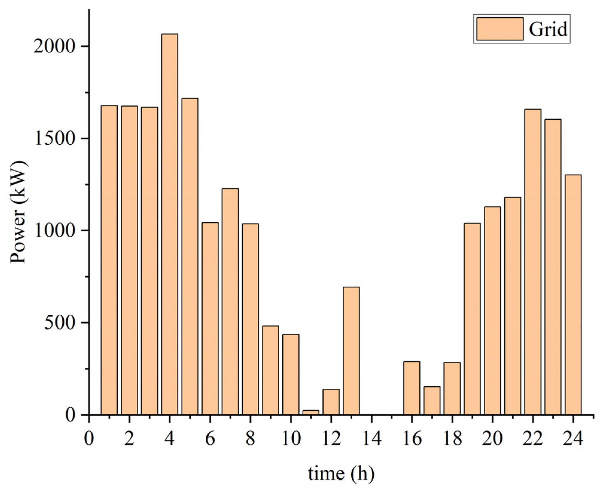
  • In hydrogen–electric coupled microgrids, the energy management system can intelligently adjust charging and discharging strategies based on electricity price signals and photovoltaic generation through the DDPG algorithm, achieving “buy low, sell high” operations.
  • The DDPG algorithm takes into account the volatility of photovoltaic generation, the uncertainties of charging/hydrogen loads, and other uncertain factors, ensuring supply–demand balance between photovoltaic generation, electric vehicle charging/hydrogen loads, and the energy storage system during the scheduling period, thus enhancing the reliability and stability of system operation.
  • Through the DDPG algorithm, hydrogen–electric coupled microgrids can participate in flexible grid regulation based on electricity price incentive signals by adjusting charging loads and energy storage systems, reducing peak loads, and improving grid stability and economic efficiency.
  • The accuracy of the DDPG algorithm in continuous action problems has been validated through comparisons with the DQN algorithm.
Future research will delve deeper into the aggregation management and coordination control strategies of multiple hydrogen–electric coupled microgrids under a virtual power plant model, exploring the scalable aggregation effects and adjustment potential of hydrogen–electric coupled microgrids to provide abundant and reliable flexible adjustment resources for new power system operations with high proportions of intermittent renewable energy.

Author Contributions

Conceptualization, T.S. (Tao Shi); methodology, T.S. (Tao Shi) and H.Z.; software, H.Z.; validation, H.Z., T.S. (Tianyu Shi) and M.Z.; formal analysis, T.S. (Tao Shi); investigation, H.Z.; resources, T.S. (Tao Shi); data curation, H.Z.; writing—original draft preparation, H.Z.; writing—review and editing, T.S. (Tao Shi); visualization, H.Z.; supervision, T.S. (Tao Shi); project administration, T.S. (Tao Shi); funding acquisition, T.S. (Tao Shi) All authors have read and agreed to the published version of the manuscript.

Funding

This research is funded by the major project of the National Natural Science Foundation of China (No. 62192753) and the Natural Science Foundation Project of Ningxia Province in China (No. 2023A1773).

Data Availability Statement

Data are contained within the article.

Conflicts of Interest

The authors declare no conflicts of interest.

References

  1. Shi, T.; Sheng, J.; Chen, Z.; Zhou, H. Simulation Experiment Design and Control Strategy Analysis in Teaching of Hydrogen-Electric Coupling System. Processes 2024, 12, 138. [Google Scholar] [CrossRef]
  2. Cai, G.; Chen, C.; Kong, L.; Peng, L.; Zhang, H. Modeling and Control of grid-connected system of wind power/photovoltaic/Hydrogen production/Supercapacitor. Power Syst. Technol. 2016, 40, 2982–2990. [Google Scholar] [CrossRef]
  3. Zhang, R.; Li, X.; Wang, X.; Wang, Q.; Qi, Z. Optimal scheduling for hydrogen-electric hybrid microgrid with vehicle to grid technology. In 2021 China Automation Congress (CAC); IEEE: Piscataway, NJ, USA, 2021; pp. 6296–6300. [Google Scholar]
  4. Guanghui, L. Research on Modeling and Optimal Control of Wind-Wind Hydrogen Storage Microgrid System. Master’s Thesis, North China University of Technology, Beijing, China, 2024. [Google Scholar]
  5. Huo, Y.; Wu, Z.; Dai, J.; Huo, Y.; Wu, Z.; Dai, J.; Duan, W.; Zhao, H.; Jiang, J.; Yao, R. An Optimal Dispatch Method for the Hydrogen-Electric Coupled Energy Microgrid. In World Hydrogen Technology Convention; Springer Nature Singapore: Singapore, 2023; pp. 69–75. [Google Scholar]
  6. Hou, L.; Dong, J.; Herrera, O.E.; Mérida, W. Energy management for solar-hydrogen microgrids with vehicle-to-grid and power-to-gas transactions. Int. J. Hydrogen Energy 2023, 48, 2013–2029. [Google Scholar] [CrossRef]
  7. Yu, L.; Qin, S.; Zhang, M.; Shen, C.; Jiang, T.; Guan, X. Deep reinforcement learning for smart building energy management: A survey. arXiv 2020, arXiv:2008.05074. [Google Scholar]
  8. Zheng, J.; Song, Q.; Wu, G.; Chen, H.; Hu, Z.; Chen, Z.; Weng, C.; Chen, J. Low-carbon operation strategy of regional integrated energy system based on the Q learning algorithm. J. Electr. Power Sci. Technol. 2022, 37, 106–115. [Google Scholar]
  9. Xu, H.; Lu, J.; Yang, Z.; Li, Y.; Lu, J.; Huang, H. Decision optimization model of incentive demand response based on deep reinforcement learning. Autom. Electr. Power Syst. 2021, 45, 97–103. [Google Scholar]
  10. Shuai, C. Microgrid Energy Management and Scheduling Based on Reinforcement Learning. Ph.D. Thesis, University of Science and Technology Beijing, Beijing, China, 2023. [Google Scholar]
  11. Kim, B.; Zhang, Y.; Van Der Schaar, M.; Lee, J.W. Dynamic pricing and energy consumption scheduling with reinforcement learning. IEEE Trans. Smart Grid 2016, 7, 2187–2198. [Google Scholar] [CrossRef]
  12. Shi, T.; Xu, C.; Dong, W.; Zhou, H.; Bokhari, A.; Klemeš, J.J.; Han, N. Research on energy management of hydrogen electric coupling system based on deep reinforcement learning. Energy 2023, 282, 128174. [Google Scholar] [CrossRef]
  13. Liu, J.; Chen, J.; Wang, X.; Zeng, J.; Huang, Q. Research on Energy Management and Optimization Strategy of micro-energy networks based on Deep Reinforcement Learning. Power Syst. Technol. 2020, 44, 3794–3803. [Google Scholar] [CrossRef]
  14. Ji, Y.; Wang, J.; Xu, J.; Fang, X.; Zhang, H. Real-Time Energy Management of a Microgrid Using Deep Reinforcement Learning. Energies 2019, 12, 2291. [Google Scholar] [CrossRef]
  15. Darshi, R.; Shamaghdari, S.; Jalali, A.; Arasteh, H. Decentralized Reinforcement Learning Approach for Microgrid Energy Management in Stochastic Environment. Int. Trans. Electr. Energy Syst. 2023, 2023, 1190103. [Google Scholar] [CrossRef]
  16. Kolodziejczyk, W.; Zoltowska, I.; Cichosz, P. Real-Time Energy Purchase Optimization for a Storage-Integrated Photovoltaic System by Deep Reinforcement Learning. Control Eng. Pract. 2021, 106, 104598. [Google Scholar] [CrossRef]
  17. Nicola, M.; Nicola, C.I.; Selișteanu, D. Improvement of the Control of a Grid Connected Photovoltaic System Based on Synergetic and Sliding Mode Controllers Using a Reinforcement Learning Deep Deterministic Policy Gradient Agent. Energies 2022, 15, 2392. [Google Scholar] [CrossRef]
  18. Wang, C.; Zhang, J.; Wang, A.; Wang, Z.; Yang, N.; Zhao, Z.; Lai, C.S.; Lai, L.L. Prioritized sum-tree experience replay TD3 DRL-based online energy management of a residential microgrid. Appl. Energy 2024, 368, 123471. [Google Scholar] [CrossRef]
  19. Guo, C.; Wang, X.; Zheng, Y.; Zhang, F. Real-time optimal energy management of microgrid with uncertainties based on deep reinforcement learning. Energy 2022, 238, 121873. [Google Scholar] [CrossRef]
  20. Benhmidouch, Z.; Moufid, S.; Ait-Omar, A.; Abbou, A.; Laabassi, H.; Kang, M.; Chatri, C.; Ali, I.H.O.; Bouzekri, H.; Baek, J. A novel reinforcement learning policy optimization based adaptive VSG control technique for improved frequency stabilization in AC microgrids. Electr. Power Syst. Res. 2024, 230, 110269. [Google Scholar] [CrossRef]
Figure 1. A typical structure of a hydrogen–electric coupling microgrid.
Electronics 13 03389 g001
Figure 2. Structure of the DDPG algorithm.
Electronics 13 03389 g002
Figure 3. Typical curves of solar photovoltaic output, charging load forecast, and hydrogen charging load forecast.
Electronics 13 03389 g003
Figure 4. Pricing signal.
Electronics 13 03389 g004
Figure 5. Energy management strategy reward convergence curve.
Electronics 13 03389 g005
Figure 6. Hydrogen tank and electrical energy storage system operational strategies.
Electronics 13 03389 g006
Figure 7. The charging strategy for microgrids.
Electronics 13 03389 g007
Figure 8. Hydrogen loading strategies for microgrids under different algorithms.
Electronics 13 03389 g008
Figure 9. The purchasing strategy of microgrids from the public electricity grid.
Electronics 13 03389 g009
Table 1. Description of a regional hydrogen–electric coupled microgrid.
ParameterValues
Photovoltaic array600 kW
Capacity of electrical energy storage system72–288 kW·h
Electrical energy storage power rating100 kW
Electrolyzer rated power750 kW
Capacity of hydrogen storage tank1000 Nm3
Capacity of charging30 × 30 kW
Total refueling rate30 × 5 Nm3/h
Batch size64
Hydrogen refueling service price5.8 ¥/Nm3
Carbon trading price0.07 ¥/kg
Table 2. Parameter configuration.
ParameterValues
Hidden layer[400, 300, 256, 128]
Actor network learning rate0.001
Critic network learning rate0.001
Target network learning rate0.001
Discount factor0.99
Episodes1000
Step size100
Batch size64
Experience playback pool capacity20,000
Hidden layer[400, 300, 256, 128]
Actor network learning rate0.001
Table 3. Operating costs of hydrogen–electric coupled microgrids under various conditions.
Cost (CNY)Before OptimizationDQNDDPG
Power purchase cost9625.279038.198677.2
Charging income8056.337783.617838.3
Hydrogen charge yield11,314.7911,201.642111,314.79
Carbon revenue147.89147.89147.89
Net revenue9893.7410,094.952110,623.78
Disclaimer/Publisher’s Note: The statements, opinions and data contained in all publications are solely those of the individual author(s) and contributor(s) and not of MDPI and/or the editor(s). MDPI and/or the editor(s) disclaim responsibility for any injury to people or property resulting from any ideas, methods, instructions or products referred to in the content.

