Evaluation Approach and Controller Design Guidelines for Subsequent Commutation Failure in Hybrid Multi-Infeed HVDC System

Abstract

Due to the difference in output characteristics between the line-commutated converter-based high-voltage direct current (LCC-HVDC) and voltage-source converter-based high-voltage direct current (VSC-HVDC), the hybrid multi-infeed high-voltage direct current (HMIDC) presents complex coupling characteristics. As the AC side is disturbed, the commutation failure (CF) occurring on the LCC side is the main factor threatening the safe operation of the system. In this paper, the simplified equivalent network model of HMIDC is established by analyzing the output characteristics of VSC and LCC. Hereafter, based on the derived model and the control system of LCC-HVDC, the dynamic equations of the extinction angle are deduced. Consequently, by applying the phase portrait method, the causes of CF occurring in the HMIDC system as well as the impacts of control parameters on the transient stability are revealed. Furthermore, the stabilization boundaries for the reference value of the DC voltage are obtained via the above analysis. Finally, the theoretical analysis is verified by the simulations in the PSCAD/EMTDC.

1. Introduction

In recent years, the hybrid multi-infeed high-voltage direct current (HMIDC) system has been developed due to the electrical coupling between the newly penetrated voltage-source converter-based high-voltage direct current (VSC-HVDC) and the line-commutated converter-based high-voltage direct current (LCC-HVDC) already in operation [1,2,3]. For example, the Wudongde Hydropower Station employs a VSC-HVDC system and is located near the Xiluodu–Guangdong project, which has been constructed utilizing an LCC-HVDC system. Thereby, the two systems exhibit the characteristics of an HMIDC system [4]. As an AC fault occurs, the ability of the system maintaining transient stability may be impaired due to the electrical coupling between the VSC and LCC stations, as well as the power interaction between the two systems via the contact line [2,5,6].

For HMIDC systems, the occurrence of the commutation failure (CF) at the LCC side due to AC disturbances is a major threat to the stable operation of the system [7], and with system self-regulation, the first commutation failure (FCF) will recover quickly after it occurs; in contrast, the subsequent commutation failure (SCF) following the FCF is a greater threat [8].

For the stability of the HMIDC system, the small-signal analysis is generally applied to reveal the interaction dynamics between VSC-HVDC and LCC-HVDC [6]. Through the eigenvalue analysis and participating analysis, ref. [9] identified the inherent oscillatory modes of the HMIDC system, while clarifying the impact of the crucial controller parameters on system damping. Based on the individual channel analysis and design (ICAD) theory, ref. [10] proposed an equivalent single-input–single-output (SISO) feedback control model for the HIMDC system. Consequently, the impacts of the AC system strength and control system on the system stability can be evaluated via the gain margin (GM) and phase margin (PM) indexes. Nonetheless, as the AC system is subjected to large disturbances deviating from the equilibrium point (EP), the small-signal model based on the linearization near the EP is not applicable [11].

There are numerous transient characterization efforts for large disturbances occurring in HMIDC systems, as well as many indexes to assess the risk of CFs occurring in HMIDC systems. In general, the strength of the system is closely related to the occurrence of the CFs. Specifically, the stronger the strength of the system, the better support provided to the LCC inverter during an AC fault, resulting in a lower risk of CF [12]. For the LCC-HVDC systems, the effective short-circuit ratio (ESCR) strength index based on the commutation voltage-time area theory is proposed to assess the risk of CF, as there is an approximately linear correlation between the risk of CF and the index [13,14], whereas the ESCR cannot be directly applied to evaluate the strength of the HMIDC system due to the distinct output characteristics of the VSC and LCC, as well as the inability to apply the communication voltage-time area theory to the VSC [12]. Subsequently, an approach is proposed in [15] to effectively identify buses in HMIDC systems with potential CFs. It involves real-time calculation for the AC–DC system voltage interaction factor utilizing LCC receiving-end voltages and system parameters to predict the location of CFs. To further analyze the interaction effects between VSC and LCC in HMIDC systems, ref. [16] introduces the multi-infeed voltage interaction factor (MVIF) index, which is capable of assessing the voltage interaction effect among individual converters. Additionally, ref. [17] defines an equivalent voltage stability indicator (EVSI) based on the equivalent analytical model of HMIDC, which facilities the calculation of the CF immunity index (CFII) to assess the risk of CFs. In [18], the concept of virtual impedance is applied to equate the multilinked HVDC system to a single-infeed system, and then the unified ESCR (UESCR) is proposed to evaluate the strength of the new system. In [19], the short-term voltage stability constraints (SVSCUC) index for evaluating the voltage support capacity and voltage stability in the HMIDC system is proposed. Further, compared to the VSC employing constant reactive power control, the VSC utilizing a constant AC voltage controller yields a more significant improvement in CFII [20]. Moreover, the improvement effect is directly related to the speed at which the controller operates. Besides that, there are still other indicators for optimizing the effect of CFII in the HIMDC system. For instance, in [21], the critical voltage correlation factor (CVCF) that can reasonably select the location of the dynamic reactive power compensation device was proposed to enhance the effect of CFII. Yet, these assessment indexes fail to intuitively describe the transient process in HMIDC systems and are not sufficient to reveal the mechanism of SCF occurrence.

To present the transient process more intuitively, this paper establishes the equivalent port network model of the HMIDC system and identifies the key system parameters influencing CF by integrating this model with the system’s transient change process. Subsequently, the dynamic equation of the shut-off angle is established based on the LCC control system, and the crucial controller parameters affecting the risk of CFs and corresponding stability boundary are analyzed by the phase portrait method. Finally, the theoretical analysis is validated by the simulations in PSCAD/EMTDC.

2. Mathematical Model of the HMIDC System

2.1. System Description

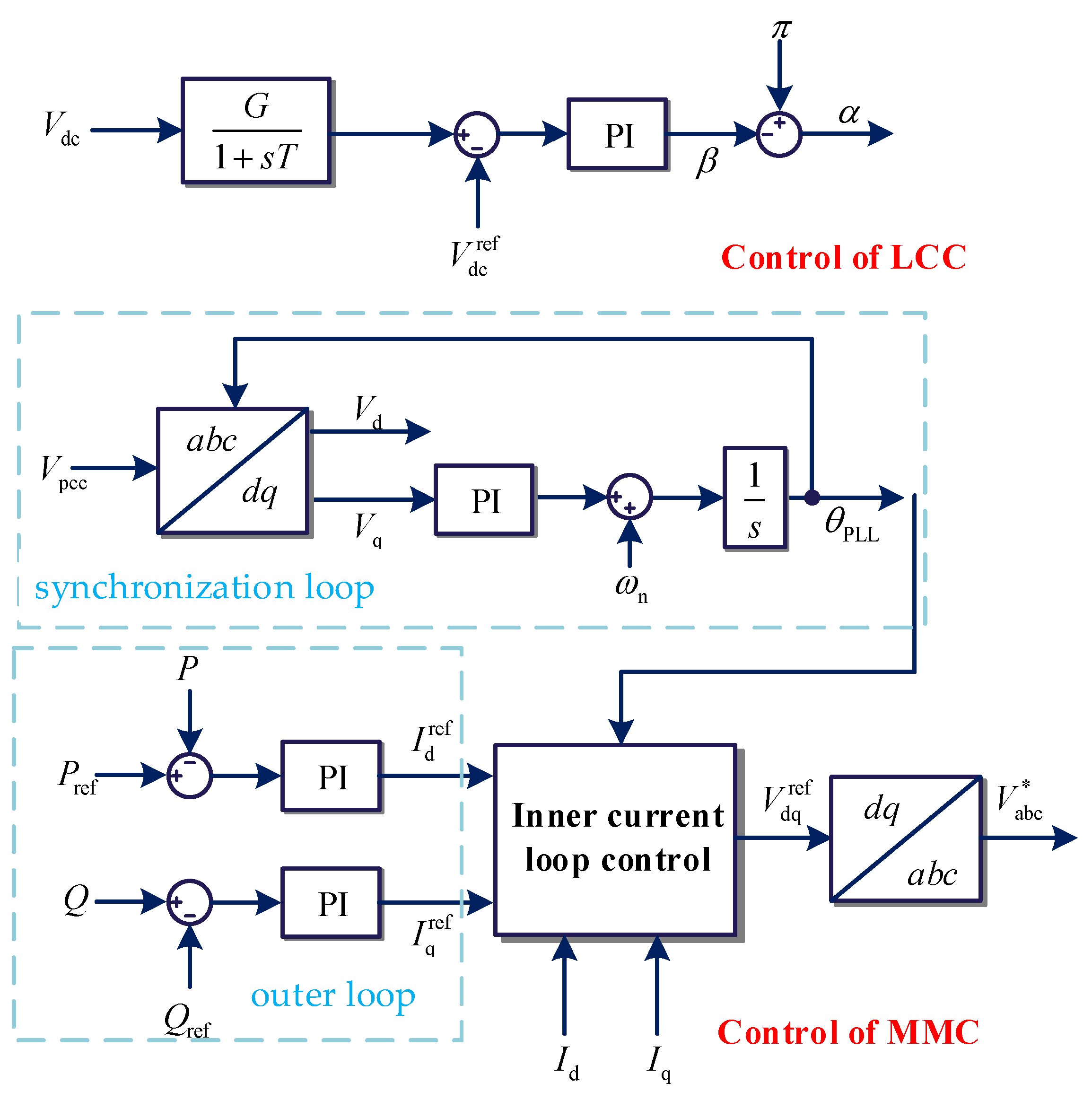
The structure of the HMIDC system is shown in Figure 1, where $I_{\mathrm{d}\mathrm{c}}^{\mathrm{L}\mathrm{C}\mathrm{C}}$ denotes the DC current of the LCC inverter controlled by the rectifier of the LCC-HVDC system. $V_{\mathrm{d}\mathrm{c}}^{\mathrm{M}\mathrm{M}\mathrm{C}}$ denotes the DC voltage of the MMC inverter, which is controlled by the rectifier of the MMC-HVDC system. As the inverters at the receiving end of the LCC and MMC, both of them are connected to the equivalent grid through the line impedance and also are connected to each other through the contact line. In addition, filters are provided at Bus1 to eliminate harmonics and provide reactive power support to the LCC inverter.

2.2. Power Control

The control structure of the HMIDC system is shown in Figure 2. The constant DC voltage control is applied to the LCC inverter to keep the DC voltage of the LCC constant, while the MMC inverter adopts the grid-following control to keep the power output constant.

The mathematical model of LCC inverter controller is as follows:

$$\left\{\begin{array}{l}\beta =({\displaystyle \frac{G}{1+sT}}{V}_{\mathrm{dc}}-V_{\mathrm{dc}}^{\mathrm{ref}})(k_{\mathrm{p}}^{\mathrm{t}1}+k_{\mathrm{i}}^{\mathrm{t}1}/s)\\ \alpha =\pi -\beta \end{array}\right.$$

(1)

where α and β denote the trigger angle of the LCC as well as the advanced trigger; V_dc and $V_{\mathrm{dc}}^{\mathrm{ref}}$ denote the DC voltage and its reference value, respectively; and $k_{\mathrm{p}}^{\mathrm{t}1}$ and $k_{\mathrm{i}}^{\mathrm{t}1}$ denote the parameters of the DC voltage controller.

For the LCC inverter, when the commutation process is ignored, the operating characteristics can be expressed as

$$\left\{\begin{array}{l}{V}_{\mathrm{dc}}={\displaystyle \frac{3\sqrt{2}Nk}{\pi }}{U}_{\mathrm{LN}}\cos \gamma -I_{\mathrm{dc}}{R}_{\mathrm{c}}\\ I_{\mathrm{LN}}={\displaystyle \frac{N2\sqrt{3}k}{\pi }}{I}_{\mathrm{dc}}\\ \phi =\arccos (\cos \beta +{\displaystyle \frac{I_{\mathrm{dc}}{X}_{\mathrm{c}}}{\sqrt{3}k{U}_{\mathrm{LN}}}})\end{array}\right.$$

(2)

where N denotes the number of six-pulsed LCC valves connected in series on the inverter side, and is generally set to 2. U_LN and I_LN are the amplitude of AC measured phase voltage and current, respectively. Rc and Xc denote the equivalent commutation resistance and reactance, respectively. φ denotes the output power factor angle of the inverter, and k represents the transformer ratio.

Based on the controller structure of MMC shown in Figure 2, the current reference in the dq-axis is derived as

$$\left\{\begin{array}{l}{I}_{\mathrm{d}}^{\mathrm{ref}}=(P_{\mathrm{ref}}-P)(k_{\mathrm{p}}^{\mathrm{t}2}+k_{\mathrm{i}}^{\mathrm{t}2}/s)\\ I_{\mathrm{q}}^{\mathrm{ref}}=(Q-Q_{\mathrm{ref}})(k_{\mathrm{p}}^{\mathrm{t}2}+k_{\mathrm{i}}^{\mathrm{t}2}/s)\end{array}\right.$$

(3)

where P_ref and Q_ref denote the reference values of active and reactive power for the MMC output, and $k_{\mathrm{p}}^{\mathrm{t}2}$ and $k_{\mathrm{i}}^{\mathrm{t}2}$ denote the control parameters of the PLL.

For the synchronization control loop in the MMC rectifier, the phase-locked loop (PLL) is employed, and the output phase θ_PLL can be derived as

$${\theta }_{\mathrm{PLL}}={\displaystyle \frac{1}{s}}[V_{\mathrm{PCC}}^{\mathrm{q}}(k_{\mathrm{p}}+k_{\mathrm{i}}/s)+{\omega }_{\mathrm{n}}]$$

(4)

where θ_PLL denotes the phase of the PLL output; ω_n corresponds to the reference frequency; and $V_{\mathrm{PCC}}^{\mathrm{q}}$ denotes the Q-axis component of the AC voltage in the coordinate system of the PLL, which is equal to zero at steady state.

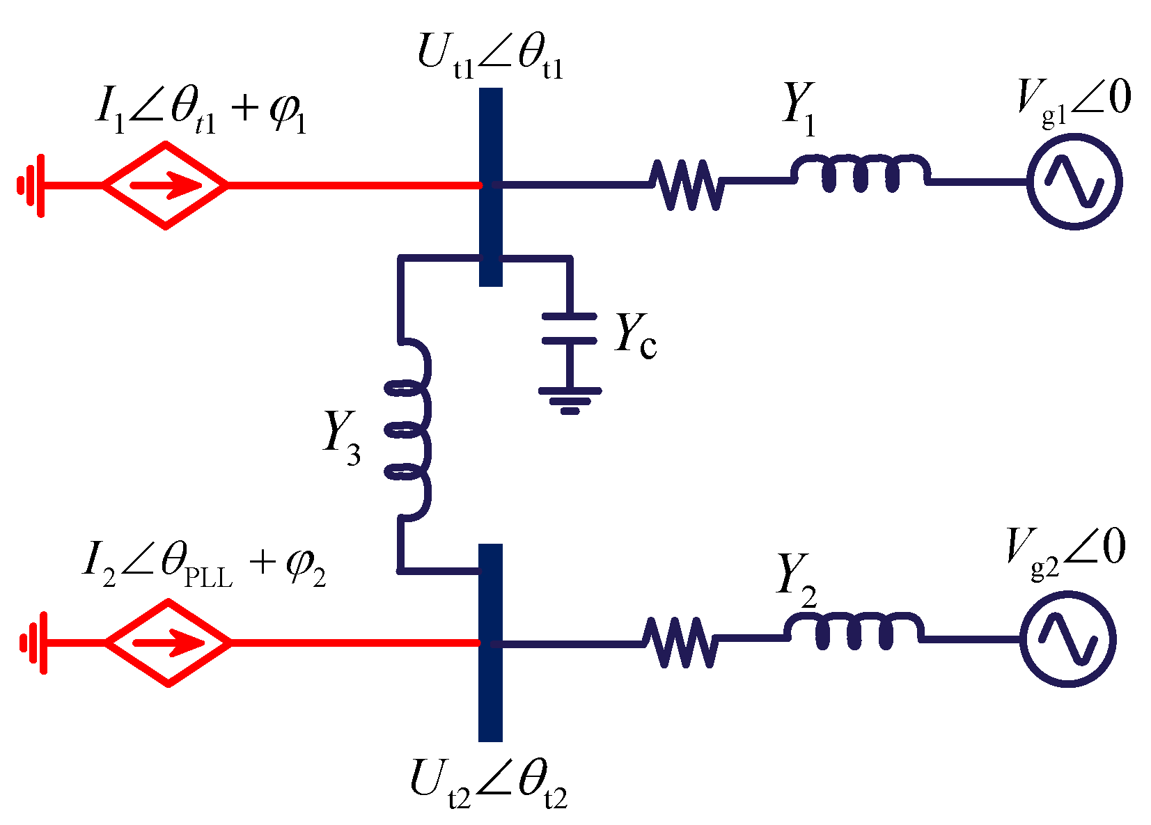
2.3. Equivalent Modeling Network for HMIDC Systems

From the above analysis, the MMC rectifier operated in the grid-following control can be equivalent to the controlled current source, whose amplitude and phase are determined by the output of the PLL and the inner current control loop. Similarly, the LCC inverter can also be equivalent to a current source since its DC current is controlled to a constant value. The power factor angle of the LCC is related to the output of the controller output, so it can be equated to a current source that always exceeds the phase of the AC bus by angle φ. Therefore, the equivalent circuit of the HMIDC system can be depicted by Figure 3.

In Figure 3, Yc is the equivalent conductance of the filter, and the line impedances are denoted by Y₁, Y₂, and Y₃. Taking the phase of the AC grid as a reference, the model of the equivalent current source at the LCC terminal is denoted as

$$\left\{\begin{array}{l}{I}_1={\displaystyle \frac{4\sqrt{3}}{\pi }}k{i}_{\mathrm{dc}}\\ {\phi }_1=\arccos (\cos \beta +{\displaystyle \frac{I_{\mathrm{dc}}{X}_{\mathrm{c}}}{\sqrt{3}k{U}_{\mathrm{t}1}}})\end{array}\right.$$

(5)

Equation (5) indicates that the amplitude of the current source is determined by the DC current i_dc, while its phase deviates from the AC bus by ${\phi }_1$. Meanwhile, the equivalent current source at the MMC side is expressed as

$$\left\{\begin{array}{l}{I}_2=\sqrt{I_{\mathrm{d}}^2+I_{\mathrm{q}}^2}\\ {\phi }_2=\arctan ({\displaystyle \frac{I_{\mathrm{q}}}{I_{\mathrm{d}}}})\end{array}\right.$$

(6)

Equation (6) shows that the MMC with the grid-following control is equivalent to a current source, and its amplitude is determined by the magnitude of the dq-axis current. ${\phi }_2$ is the phase deviation between θ_PLL and AC bus. According to the KCL and KVL theorems, the nodal admittance equations shown in Figure 3 can be derived as

$$\left\{\begin{array}{l}{\mathit{I}}_1={\mathit{U}}_{\mathbf{t}1}{\mathit{Y}}_{\mathbf{c}}+({\mathit{U}}_{\mathbf{t}1}-{\mathit{U}}_{\mathbf{t}2}){\mathit{Y}}_3+({\mathit{U}}_{\mathbf{t}1}-{\mathit{U}}_{\mathbf{g}1}){\mathit{Y}}_1\\ {\mathit{I}}_2=({\mathit{U}}_{\mathbf{t}2}-{\mathit{U}}_{\mathbf{t}1}){\mathit{Y}}_3+({\mathit{U}}_{\mathbf{t}2}-{\mathit{U}}_{\mathbf{g}2}){\mathit{Y}}_2\end{array}\right.$$

(7)

By representing the variables in the matrix form, Equation (7) is modified as

$$\left[\begin{array}{c}{\mathit{I}}_1\\ {\mathit{I}}_2\end{array}\right]=\left[\begin{array}{cc}{\mathit{Y}}_{11}& {\mathit{Y}}_{12}\\ {\mathit{Y}}_{21}& {\mathit{Y}}_{22}\end{array}\right]\left[\begin{array}{c}{\mathit{U}}_{\mathbf{t}1}\\ {\mathit{U}}_{\mathbf{t}2}\end{array}\right]-\left[\begin{array}{c}{\mathit{G}}_1\\ {\mathit{G}}_2\end{array}\right]$$

(8)

The elements in Equation (8) are expressed as

$$\left\{\begin{array}{l}{\mathit{Y}}_{11}={\mathit{Y}}_{\mathbf{c}}+{\mathit{Y}}_1+{\mathit{Y}}_3\\ {\mathit{Y}}_{12}=-{\mathit{Y}}_3\\ {\mathit{Y}}_{21}=-{\mathit{Y}}_3\\ {\mathit{Y}}_{22}={\mathit{Y}}_2+{\mathit{Y}}_3\\ {\mathit{G}}_1={\mathit{Y}}_1{\mathit{U}}_{\mathbf{g}1}\\ {\mathit{G}}_2={\mathit{Y}}_2{\mathit{U}}_{\mathbf{g}2}\end{array}\right.$$

(9)

3. Dynamic Characterization of HMIDC Systems under Grid Faults

For LCC inverters, the system is at risk of CFs as the AC side fails to provide sufficient support due to grid fault occurrence. It is widely recognized that the commutation failure will occur at the inverter station in the LCC-HVDC system as the extinction angle γ is less than the critical extinction angle ${\gamma }_{\mathrm{m}\mathrm{i}\mathrm{n}}$, which is generally 10° [22]. Meanwhile, it is assumed that the first commutation failure (FCF) is recovered quickly by self-regulation [16]. Therefore, the mechanism of subsequent commutation failure (SCF) and suppression strategies should be analyzed in detail.

In the HMIDC system, the dynamic characteristics of the LCC inverter are also affected by the MMC rectifier when a grid fault occurs at the LCC side due to the electrical coupling.

For the LCC inverter, the mathematical relationship between the extinction angle $\gamma$ and the advanced trigger angle $\beta$ is expressed as

$$\beta =\arccos (\cos \gamma +{\displaystyle \frac{\sqrt{2}{I}_{\mathrm{dc}}}{k{U}_{\mathrm{t}1}}})$$

(10)

Combining Equations (1), (2) and (10) yields the following dynamic equation for the extinction angle $\gamma$.

$$\arccos (\cos \gamma +{\displaystyle \frac{\sqrt{2}{I}_{\mathrm{dc}}}{k{U}_{\mathrm{t}1}}})=(k_{\mathrm{p}}^{\mathrm{t}1}+k_{\mathrm{i}}^{\mathrm{t}1}/s)({\displaystyle \frac{6\sqrt{2}k}{\pi }}{U}_{\mathrm{t}1}\cos \gamma -I_{\mathrm{dc}}{R}_{\mathrm{c}}-V_{\mathrm{dc}}^{\mathrm{ref}})$$

(11)

Differentiating Equation (11) yields

$$\dot{\gamma }={\displaystyle \frac{k_{\mathrm{i}}^{\mathrm{t}1}(\frac{6\sqrt{2}k}{\pi }{U}_{\mathrm{t}1}\cos \gamma -I_{\mathrm{dc}}{R}_{\mathrm{c}}-V_{\mathrm{dc}}^{\mathrm{ref}})}{\frac{6\sqrt{2}k}{\pi }{U}_{\mathrm{t}1}\sin \gamma +\frac{\sin \gamma }{\sqrt{1-{(\cos \gamma +\frac{\sqrt{2}{I}_{\mathrm{dc}}}{k{U}_{\mathrm{t}1}})}^2}}}}$$

(12)

where $\dot{\gamma }$ denotes the derivative of the extinction angle $\gamma$ with respect to time.

From Equation (12), it is revealed that the dynamic characteristics of the extinction angle are related to its AC bus voltage $U_{\mathrm{t}1}$. Once $U_{\mathrm{t}1}$ is solved and combined with the value of $\gamma$ at the current moment, its dynamic characteristics can be predicted, which in turn determines whether the SCF will occur.

Between the recovery from FCF and SCF, the converter valves have returned to normal commutation, the AC voltage is maintained at some lower constant value, and the DC current changes slightly [18]. Therefore, it is assumed that $U_{\mathrm{t}1}$ remains essentially unchanged after FCF recovery. As a result, the solution for the magnitude of U_t1 after recovery from the FCF is the crucial step to assess the risk of SCF in the HMIDC system. Applying the phasor representation for the variables to Equation (8) yields

$$\left\{\begin{array}{l}{I}_1\cos ({\theta }_{\mathrm{t}1}+{\phi }_1)=y_{11}{U}_{\mathrm{t}1}\cos ({\theta }_{11}+{\theta }_{\mathrm{t}1})+y_{12}{U}_{\mathrm{t}2}\cos ({\theta }_{12}+{\theta }_{\mathrm{t}2})-g_1\cos {\theta }_{\mathrm{g}1}\\ I_1\sin ({\theta }_{\mathrm{t}1}+{\phi }_1)=y_{11}{U}_{\mathrm{t}1}\sin ({\theta }_{11}+{\theta }_{\mathrm{t}1})+y_{12}{U}_{\mathrm{t}2}\sin ({\theta }_{12}+{\theta }_{\mathrm{t}2})-g_1\sin {\theta }_{\mathrm{g}1}\\ I_2\cos ({\theta }_{\mathrm{PLL}}+{\phi }_2)=y_{21}{U}_{\mathrm{t}1}\cos ({\theta }_{11}+{\theta }_{\mathrm{t}1})+y_{22}{U}_{\mathrm{t}2}\cos ({\theta }_{22}+{\theta }_{\mathrm{t}2})-g_2\cos {\theta }_{\mathrm{g}2}\\ I_2\sin ({\theta }_{\mathrm{PLL}}+{\phi }_2)=y_{21}{U}_{\mathrm{t}1}\sin ({\theta }_{11}+{\theta }_{\mathrm{t}1})+y_{22}{U}_{\mathrm{t}2}\sin ({\theta }_{22}+{\theta }_{\mathrm{t}2})-g_2\sin {\theta }_{\mathrm{g}2}\end{array}\right.$$

(13)

Further, substituting (5) and (6) into (13) yields:

$$\left\{\begin{array}{l}{\displaystyle \frac{4\sqrt{3}}{\pi }}k{i}_{\mathrm{dc}}\cos ({\theta }_{\mathrm{t}1}+\arccos (\cos \beta +{\displaystyle \frac{I_{\mathrm{dc}}{X}_{\mathrm{c}}}{\sqrt{3}k{U}_{\mathrm{t}1}}}))=\\ y_{11}{U}_{\mathrm{t}1}\cos ({\theta }_{11}+{\theta }_{\mathrm{t}1})+y_{12}{U}_{\mathrm{t}2}\cos ({\theta }_{12}+{\theta }_{\mathrm{t}2})-g_1\cos {\theta }_{\mathrm{g}1}\\ {\displaystyle \frac{4\sqrt{3}}{\pi }}k{i}_{\mathrm{dc}}\sin ({\theta }_{\mathrm{t}1}+\arccos (\cos \beta +{\displaystyle \frac{I_{\mathrm{dc}}{X}_{\mathrm{c}}}{\sqrt{3}k{U}_{\mathrm{t}1}}}))=\\ y_{11}{U}_{\mathrm{t}1}\sin ({\theta }_{11}+{\theta }_{\mathrm{t}1})+y_{12}{U}_{\mathrm{t}2}\sin ({\theta }_{12}+{\theta }_{\mathrm{t}2})-g_1\sin {\theta }_{\mathrm{g}1}\\ \sqrt{I_{\mathrm{d}}^2+I_{\mathrm{q}}^2}\cos ({\theta }_{\mathrm{PLL}}+\arctan ({\displaystyle \frac{I_{\mathrm{q}}}{I_{\mathrm{d}}}}))=\\ y_{21}{U}_{\mathrm{t}1}\cos ({\theta }_{11}+{\theta }_{\mathrm{t}1})+y_{22}{U}_{\mathrm{t}2}\cos ({\theta }_{22}+{\theta }_{\mathrm{t}2})-g_2\cos {\theta }_{\mathrm{g}2}\\ \sqrt{I_{\mathrm{d}}^2+I_{\mathrm{q}}^2}\sin ({\theta }_{\mathrm{PLL}}+\arctan ({\displaystyle \frac{I_{\mathrm{q}}}{I_{\mathrm{d}}}}))=\\ y_{21}{U}_{\mathrm{t}1}\sin ({\theta }_{11}+{\theta }_{\mathrm{t}1})+y_{22}{U}_{\mathrm{t}2}\sin ({\theta }_{22}+{\theta }_{\mathrm{t}2})-g_2\sin {\theta }_{\mathrm{g}2}\end{array}\right.$$

(14)

where $y_{11}$~$y_{22}$ and ${\theta }_{11}$~${\theta }_{22}$ correspond to the magnitude and phase of the phasors Y₁₁~Y₂₂ in Equation (9). g₁, g₂ and ${\theta }_{\mathrm{g}1}$, ${\theta }_{\mathrm{g}2}$ denote the magnitude and phase of the phasors G₁ and G₂, respectively.

It can be seen from (14) that $U_{\mathrm{t}1}$, $U_{\mathrm{t}2}$, ${\theta }_{\mathrm{t}1}$, and ${\theta }_{\mathrm{t}2}$ can be solved by the four equations in (14) as the advanced trigger angle β and ${\theta }_{\mathrm{PLL}}$ is obtained. Once $u_{\mathrm{t}1}$ at the instant of FCF recovery can be solved, the dynamic characteristics of the extinction angle can be predicted via (12). Therefore, the solution for β and ${\theta }_{\mathrm{PLL}}$ at the instant of FCF recovery is crucial to analyze the transient characteristics of the HMIDC system.

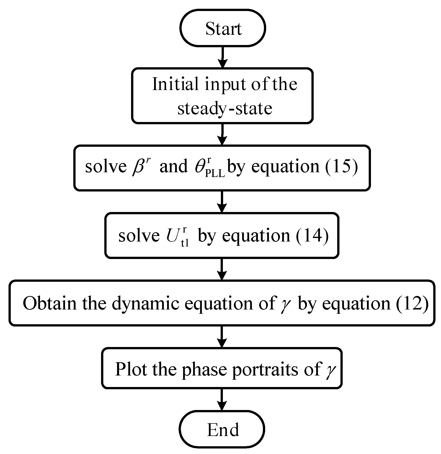
4. Transient Stability Analysis of HMIDC System Based on Phase Portraits

The variation of DC voltage of the LCC inverter when an AC fault occurs is shown in Figure 4. When the FCF happens due to a drop in the commutation voltage, the DC voltage drops rapidly to zero. Subsequently, the LCC inverter recovers from FCF under the self-regulation [19], corresponding to the instant t₂. Hereafter, as the system is controlled by inappropriate strategy, the extinction angle will again decrease below ${\gamma }_{\min }$, leading to SCF occurrence at the instant t₃.

The process of the FCF usually lasts for a short time (one duty cycle or so), and therefore, the integral part of the DC voltage controller can be assumed unchanged. Finally, the variation in β is mainly influenced by the proportional part. Also, since the ${\theta }_{\mathrm{PLL}}$ of the MMC is affected by two integral parts (as shown in Equation (4)), ${\theta }_{\mathrm{PLL}}$ can also be considered to be essentially unchanged during this short period of time.

Based on the above analysis, the expression for β and ${\theta }_{\mathrm{PLL}}$ at the instant of FCF recovery (t₂ in Figure 4) is obtained by

$$\left\{\begin{array}{l}{\beta }^{\mathrm{r}}\approx {\beta }^0-k_{\mathrm{p}}^{\mathrm{t}1}(V_{\mathrm{dc}}^{\mathrm{ref}}-0)\\ {\theta }_{\mathrm{PLL}}^{\mathrm{r}}\approx {\theta }_{\mathrm{PLL}}^0\end{array}\right.$$

(15)

where ${\beta }^{\mathrm{r}}$ and ${\beta }^0$ denote the advanced trigger angle at the instant of FCF recovery and steady state, respectively. ${\theta }_{\mathrm{P}\mathrm{L}\mathrm{L}}^{\mathrm{r}}$ and ${\theta }_{\mathrm{P}\mathrm{L}\mathrm{L}}^0$ are the ${\theta }_{\mathrm{PLL}}$ at the instant of FCF recovery and steady state, respectively.

Substituting ${\beta }^{\mathrm{r}}$ and ${\theta }_{\mathrm{P}\mathrm{L}\mathrm{L}}^{\mathrm{r}}$ into (14), r $U_{\mathrm{t}1}^{\mathrm{r}}$, $U_{\mathrm{t}2}^{\mathrm{r}}$, ${\theta }_{\mathrm{t}1}^{\mathrm{r}}$, and ${\theta }_{\mathrm{t}2}^{\mathrm{r}}$ at the instant of FCF recovery can be obtained. Further, the dynamic equation for the extinction angle γ is solved by replacing the variables in Equation (12). Consequently, the transient process between the FCF recovery and SCF occurrence can be depicted by a graphical evaluation of the $\dot{\gamma }-\gamma$ curve, which is the so-called phase portrait [23]. In this paper, the flowchart for plotting the phase portraits is shown in Figure 5.

Specifically, the phase portraits under different control parameters as $V_{\mathrm{g}1}$ drops to 0.6 p.u. are shown in Figure 6 and Figure 7.

As shown in Figure 6, when the grid voltage sags at the LCC side, the system will operate on different solid lines under different $V_{\mathrm{d}\mathrm{c}}^{\mathrm{r}\mathrm{e}\mathrm{f}}$. The points on these lines where $\dot{\gamma }=0$ represent the EP of the HMIDC system. When $\gamma ={\gamma }_{\mathrm{m}\mathrm{i}\mathrm{n}}$, the corresponding $\dot{\gamma }$ on different solid lines varies. For example, in the case of the purple solid line with $V_{\mathrm{d}\mathrm{c}}^{\mathrm{r}\mathrm{e}\mathrm{f}}=1.0\mathrm{p}.\mathrm{u}.$, the corresponding ${\dot{\gamma }}_{\min }<0$ indicates that the extinction angle will continue decreasing even if it is reduced to ${\gamma }_{\mathrm{m}\mathrm{i}\mathrm{n}}$ during the fault. Thus, the system is destabilized as the SCF occurs under this scenario [24].

To illustrate the effect of the controller parameters on SCF, Figure 7 presents the phase portrait under different k_p and k_i. It is revealed that the transient characteristics of the system can be improved by tuning the controller parameters. Specifically, the $\dot{\mathsf{\gamma }}$ corresponding to the time that $\gamma ={\gamma }_{\mathrm{m}\mathrm{i}\mathrm{n}}$ is increased as k_p increases or k_i decreases. As long as $V_{\mathrm{d}\mathrm{c}}^{\mathrm{r}\mathrm{e}\mathrm{f}}$ remains unchanged even if the controller parameters vary in a wide range, there is always: ${\dot{\gamma }}_{\mathrm{m}\mathrm{i}\mathrm{n}}<0$., Therefore, $V_{\mathrm{d}\mathrm{c}}^{\mathrm{r}\mathrm{e}\mathrm{f}}$ is the critical parameter that determines whether the SCF occurs.

In fact, from Equation (12), it can be seen that the system parameters also have an effect on the transient stability of the HMIDC system. When γ = γ_min, the derivative of the extinction angle is expressed as:

$${\dot{\gamma }}_{\min }={\displaystyle \frac{k_{\mathrm{i}}^{\mathrm{t}1}(\frac{6\sqrt{2}k}{\pi }{U}_{\mathrm{t}1}\cos {\gamma }_{\min }-I_{\mathrm{dc}}{R}_{\mathrm{c}}-V_{\mathrm{dc}}^{\mathrm{ref}})}{\frac{6\sqrt{2}k}{\pi }{U}_{\mathrm{t}1}\sin {\gamma }_{\min }+\frac{\sin \gamma }{\sqrt{1-{(\cos {\gamma }_{\min }+\frac{\sqrt{2}{I}_{\mathrm{dc}}}{k{U}_{\mathrm{t}1}})}^2}}}}$$

(16)

Due to ${\displaystyle \frac{\sqrt{2}{I}_{\mathrm{dc}}}{{kU}_{\mathrm{t}1}}}\ll \cos {\gamma }_{\min }$, it is therefore obtainable:

$$\left\{\begin{array}{l}{\displaystyle \frac{d{\dot{\gamma }}_{\min }}{d{I}_{\mathrm{dc}}}}\approx -{\displaystyle \frac{k_{\mathrm{i}}^{\mathrm{t}1}{R}_{\mathrm{c}}}{\frac{6\sqrt{2}k}{\pi }{U}_{\mathrm{t}1}\sin {\gamma }_{\min }+\frac{\sin \gamma }{\sqrt{1-{(\cos {\gamma }_{\min })}^2}}}}\\ {\displaystyle \frac{d{\dot{\gamma }}_{\min }}{d{R}_c}}\approx -{\displaystyle \frac{k_{\mathrm{i}}^{\mathrm{t}1}{I}_{\mathrm{dc}}}{\frac{6\sqrt{2}k}{\pi }{U}_{\mathrm{t}1}\sin {\gamma }_{\min }+\frac{\sin \gamma }{\sqrt{1-{(\cos {\gamma }_{\min })}^2}}}}\end{array}\right.$$

(17)

From (17), it can be seen that the larger the I_dc or R_c, the smaller the ${\dot{\gamma }}_{\min }$ and the higher the risk of SCF in the system. Therefore, lowering either I_dc or R_c is beneficial to inhibit the occurrence of SCF. Since I_dc is usually determined by the LCC rectifier and R_c is an intrinsic electrical parameter of the system [25], this paper mainly analyzes the influence of the control parameters of the LCC inverter on the stability of the HMIDC system.

Further, combining the phase portraits with Equation (12), we can obtain the boundary of the DC voltage reference $V_{\mathrm{d}\mathrm{c}}^{\mathrm{c}\mathrm{r}\mathrm{i}}$, which can ensure that the HMIDC system is not at risk of SCF during the grid transient. The voltage reference $V_{\mathrm{d}\mathrm{c}}^{\mathrm{c}\mathrm{r}\mathrm{i}}$ satisfies

$${\displaystyle \frac{k_{\mathrm{i}}^{\mathrm{t}1}(\frac{6\sqrt{2}k}{\pi }{U}_{\mathrm{t}1}^{\mathrm{r}}\cos {\gamma }_{\min }-I_{\mathrm{dc}}{R}_{\mathrm{c}}-V_{\mathrm{dc}}^{\mathrm{cri}})}{\frac{6\sqrt{2}k}{\pi }{U}_{\mathrm{t}1}^{\mathrm{r}}\sin {\gamma }_{\min }+\frac{\sin {\gamma }_{\min }}{\sqrt{1-{(\cos {\gamma }_{\min }+\frac{\sqrt{2}{I}_{\mathrm{dc}}}{k{U}_{\mathrm{t}1}^{\mathrm{r}}})}^2}}}}>0$$

(18)

5. Simulation Verification and Analysis

To verify the correctness of the above theoretical analysis and the calculated boundary value for $V_{\mathrm{d}\mathrm{c}}^{\mathrm{c}\mathrm{r}\mathrm{i}}$, the HMIDC system is constructed in PSCAD/EMTDC for verification. The system parameters are shown in

Table 1. Main parameters of the HMIDC system.

Parameter	Value	Parameter	Value
Vdc	500 kV	$k_{\mathrm{i}}^{\mathrm{t}1}$	10
Idc	1 kA	$P_{\mathrm{r}\mathrm{e}\mathrm{f}}$	1 kMW
Xc	13.57 Ω	$Q_{\mathrm{r}\mathrm{e}\mathrm{f}}$	0 kMVar
$k_{\mathrm{p}}^{\mathrm{t}1}$	0.1	$k_{\mathrm{p}}^{\mathrm{t}2}$	22
$k_{\mathrm{i}}^{\mathrm{t}2}$	100	$V_{\mathrm{g}1}$$, V_{\mathrm{g}2}$	500 kV

.

The AC grid V_g1 of the LCC drops to 0.6 p.u. at 2 s. According to the aforementioned calculation process, the maximum boundary of $V_{\mathrm{d}\mathrm{c}}^{\mathrm{c}\mathrm{r}\mathrm{i}}$ with $V_{\mathrm{g}1}=0.6 \mathrm{p}.\mathrm{u}.$ is 0.84 p.u. based on (16). Meanwhile, $V_{\mathrm{d}\mathrm{c}}^{\mathrm{r}\mathrm{e}\mathrm{f}}$ is also set to various values during faults to verify the correctness of the analysis. The results of the test are shown in Figure 8 and Figure 9.

First, the waveforms of U_t1 in Figure 8b and Figure 9b indicate that when an AC fault occurs at the LCC terminal, the bus voltage remains essentially unchanged after a rapid decrease, which is consistent with the assumptions. Secondly, since the $V_{\mathrm{dc}}^{\mathrm{ref}}$ in Figure 9 is larger than the calculated maximum boundary $V_{\mathrm{d}\mathrm{c}}^{\mathrm{c}\mathrm{r}\mathrm{i}}$, the SCF occurs, resulting in a reduction of the DC voltage to zero and destabilization of the HMIDC system. Conversely, the $V_{\mathrm{dc}}^{\mathrm{ref}}$ in Figure 8 is maintained within the boundary value $V_{\mathrm{d}\mathrm{c}}^{\mathrm{c}\mathrm{r}\mathrm{i}}$, and the system is not at risk of SCF, which verifies the accuracy of the calculated stabilization boundary value.

In order to weigh the advantages of the method proposed in this paper, the study in this paper is compared with other studies in the literature, and the results are shown in

Table 2. Comparative results of various methods.

Research Methods	Method I	Method II	Method III	Method IV	Method V
Suitable for large disturbances	√	√	×	×	√
Consideration of control systems	×	×	√	√	√
Stabilizing design guidelines	×	×	√	√	√

.

In Table 2, Method I represents the ADVIF and CADVIF indicator prediction methods proposed in [15]; Method II represents the improved CFII indicator prediction method proposed in [12]; Method III represents the damping coefficient analysis method and additional damping controller proposed in [4]; Method IV denotes the SISO equivalent model analysis method proposed in [10]; and Method V denotes the method proposed in this paper. It can be seen that the approach in this paper has the advantage of considering the role of the control system while overcoming the disadvantage that small-signal modeling cannot be applied to large perturbations [4,10], and gives guidelines for parameter design to ensure the stability of the HMIDC system during transient processes.

6. Conclusions

In this paper, the equivalent port network of the HMIDC system is established. By analyzing the dynamic equations of the LCC’s turn-off angle, it is clarified that the key to whether or not SCF occurs is its AC voltage. Then, the AC voltage during the period from FCF recovery to SCF occurrence is calculated based on the proposed equivalent model. Next, the transient stability of the HMIDC system is analyzed in conjunction with the phase portraits and the mentioned dynamic equations. Finally, the maximum DC reference voltage boundary of the LCC without SCF is calculated, the theoretical analysis is verified by simulation in PSCAD/EMTDC, and the following conclusions are obtained:

(1)

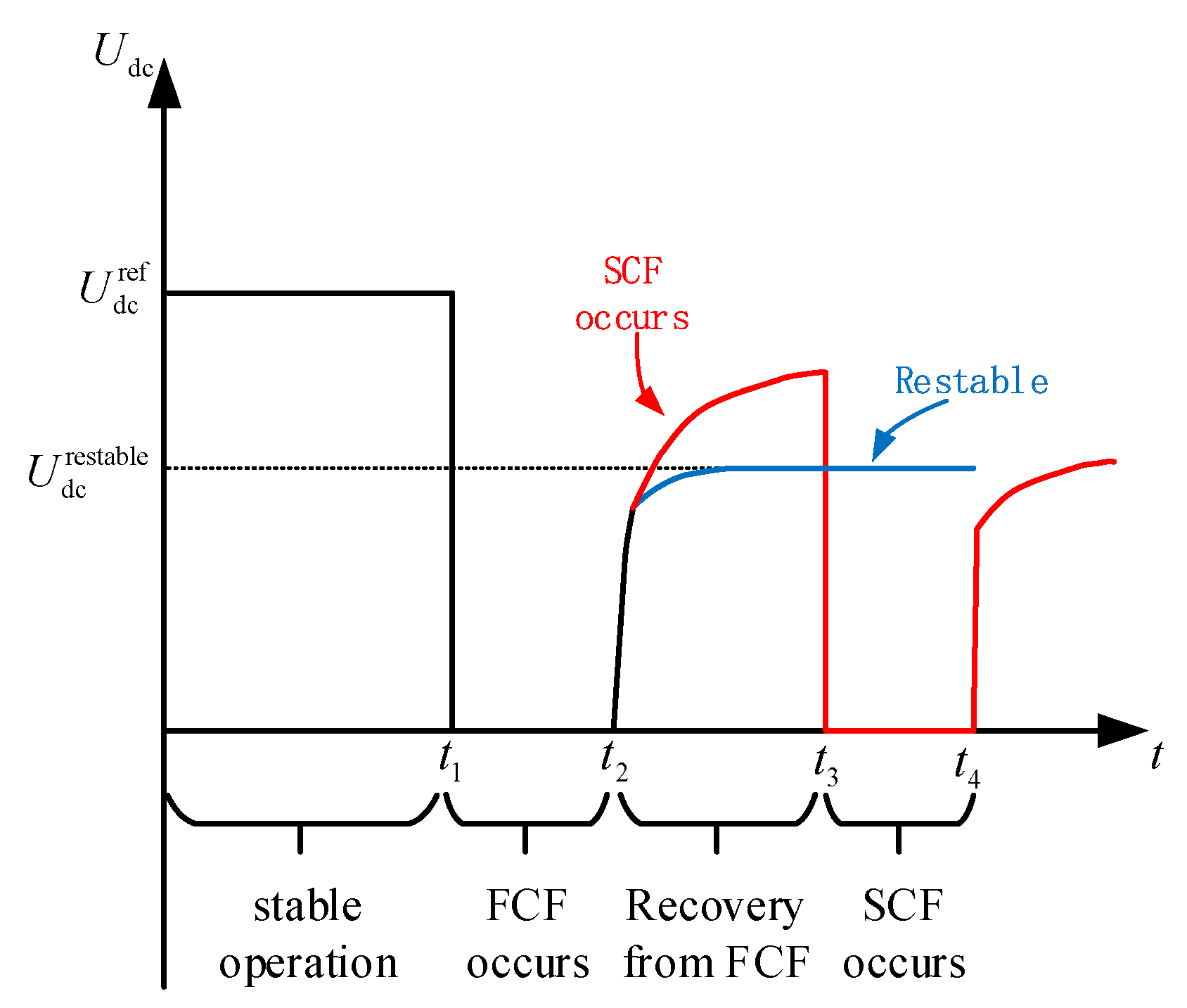
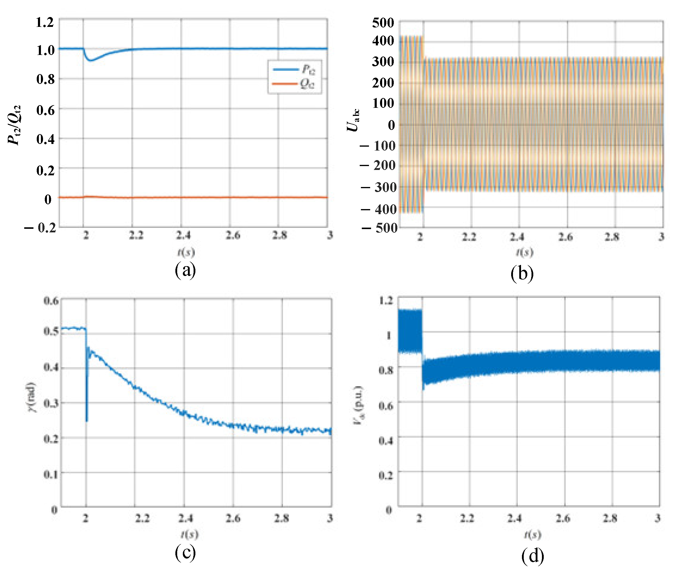
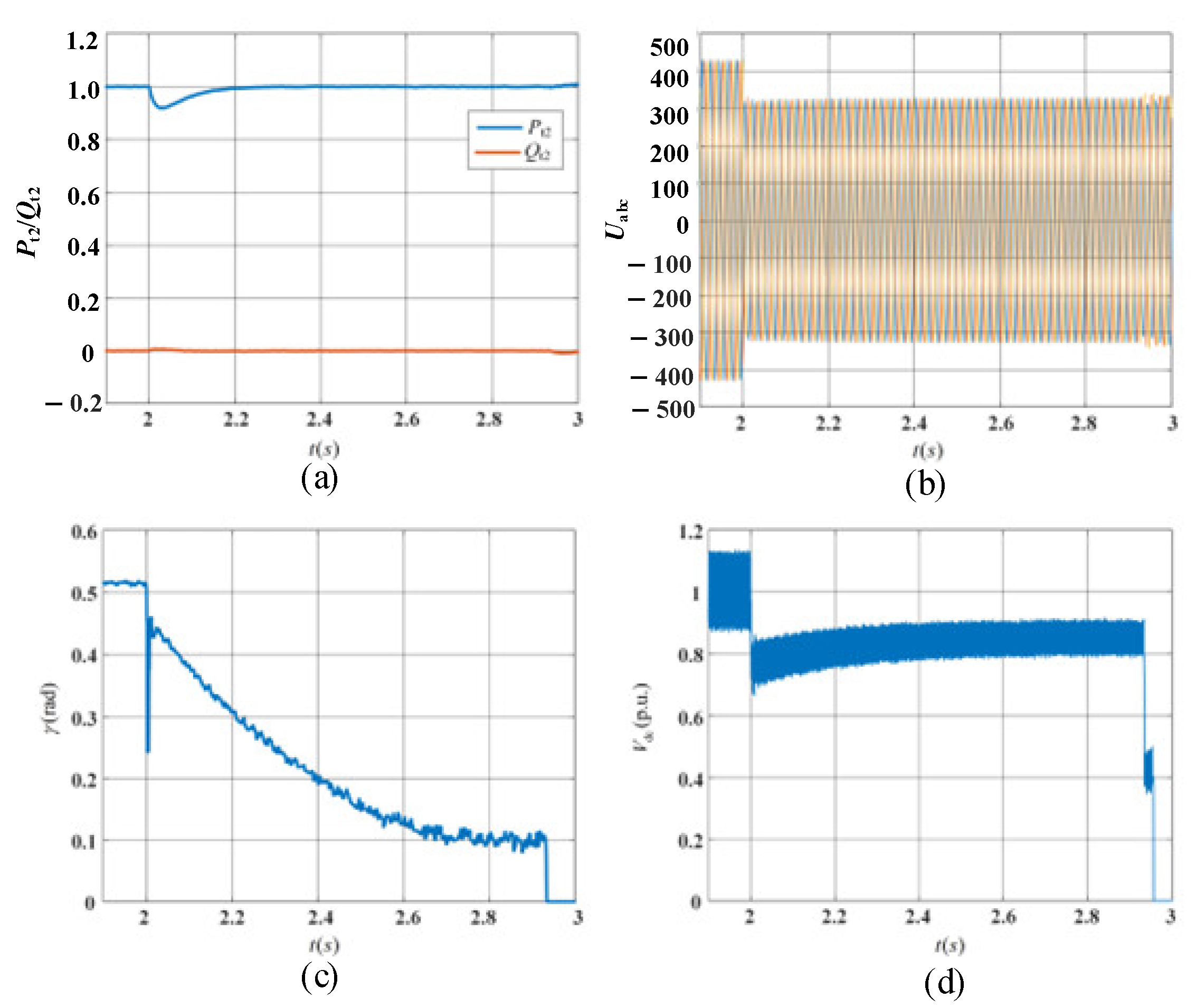
The SCF occurs in HMIDC because when the $\gamma$ keeps decreasing to its critical value under the control system, the $\dot{\gamma }$ at this point is still less than zero, which indicates that it will continue to decrease to the point at which SCF occurs.

(2)

For the LCC inverter with a constant DC voltage controller in the HMIDC system, although changing the parameters of the PI controller has an improved effect on preventing the occurrence of SCF, the decisive role is played by $V_{\mathrm{dc}}^{\mathrm{ref}}$; if $V_{\mathrm{r}\mathrm{e}\mathrm{f}}^{\mathrm{d}\mathrm{c}}$ is not changed but only the parameters of the PI controller are changed, SCF will still occur.

References

1. Guo, J.; Chen, Y.; Liao, S.; Wu, W.; Wang, X.; Guerrero, J.M. Low-Frequency Oscillation Analysis of VSM-Based VSC-HVDC Systems Based on the Five-Dimensional Impedance Stability Criterion. IEEE Trans. Ind. Electron. 2022, 69, 3752–3763. [Google Scholar] [CrossRef]
2. Guo, C.; Zhang, Y.; Gole, A.M.; Zhao, C. Analysis of dual-infeed HVDC with LCC-HVDC and VSC-HVDC. IEEE Trans. Power Del. 2012, 27, 1529–1537. [Google Scholar] [CrossRef]
3. Zhou, X.; Chen, S.; Lu, Z. Technology Features of the New Generation Power System in China. Proc. CSEE 2018, 38, 1893–1904+2205. [Google Scholar]
4. Yin, H.; Zhou, X.; Liu, Y.; Xia, H.; Hong, L.; Zhu, R.; Deng, L. Interaction Mechanism Analysis and Additional Damping Control for Hybrid Multi-Infeed HVDC System. IEEE Trans. Power Del. 2022, 37, 3904–3916. [Google Scholar] [CrossRef]
5. Lu, J.; Yuan, X.; Hu, J.; Zhang, M.; Yuan, H. Motion Equation Modeling of LCC-HVDC Stations for Analyzing DC and AC Network Interactions. IEEE Trans. Power Deliv. 2020, 35, 1563–1574. [Google Scholar] [CrossRef]
6. Wang, L.; Yang, Z.; Lu, X.; Prokhorov, A.V. Stability analysis of a hybrid multi-infeed HVDC system connected between two offshore wind farms and two power grids. IEEE Trans. Ind. Appl. 2017, 53, 1824–1833. [Google Scholar] [CrossRef]
7. Cheng, B.; Xu, Z.; Xu, W. Optimal dc-segmentation for multi-infeed HVDC systems based on stability performance. IEEE Trans. Power Syst. 2016, 31, 2445–2454. [Google Scholar] [CrossRef]
8. Guo, C.; Ye, Q.; Chen, X.; Zhao, C. Subsequent commutation failure suppression control for LCC-HVDC system based on fuzzy clustering. CSEE J. Power Energy Syst. 2024, 1–9. [Google Scholar] [CrossRef]
9. Guo, C.; Liu, W.; Zhao, J.; Zhao, C. Impact of Control System on Small-Signal Stability of Hybrid Multi-Infeed HVDC system. IET Gener. Transm. Distrib. 2018, 12, 4233–4239. [Google Scholar] [CrossRef]
10. Guo, C.; Yang, S.; Liu, W.; Zhao, C. Single-Input–Single-Output Feedback Control Model and Stability Margin Analysis for Hybrid Dual-Infeed HVDC System. IEEE J. Emerg. Sel. Top. Power Electron. 2021, 9, 3061–3071. [Google Scholar] [CrossRef]
11. Luo, C.; Liu, T.; Wang, X.; Ma, X. Design-Oriented Analysis of DC-Link Voltage Control for Transient Stability of Grid-Forming Inverters. IEEE Trans. Ind. Electron. 2024, 71, 3698–3707. [Google Scholar] [CrossRef]
12. Xiao, H.; Duan, X.; Zhang, Y.; Lan, T.; Li, Y. Analytically Quantifying the Impact of Strength on Commutation Failure in Hybrid Multi-Infeed HVdc Systems. IEEE Trans. Power Electron. 2022, 37, 4962–4967. [Google Scholar] [CrossRef]
13. Chen, X.; Gole, A.M.; Han, M. Analysis of mixed inverter/rectifier multi-infeed HVDC systems. IEEE Trans. Power Del. 2012, 27, 1565–1573. [Google Scholar] [CrossRef]
14. Hong, L.; Zhou, X.; Liu, Y.; Xia, H.; Yin, H.; Chen, Y.; Zhou, L.; Xu, Q. Analysis and Improvement of the Multiple Controller Interaction in LCC-HVDC for Mitigating Repetitive Commutation Failure. IEEE Trans. Power Deliv. 2021, 36, 1982–1991. [Google Scholar] [CrossRef]
15. Shao, Y.; Tang, Y. Fast Evaluation of Commutation Failure Risk in Multi-Infeed HVDC Systems. IEEE Trans. Power Syst. 2018, 33, 646–653. [Google Scholar] [CrossRef]
16. Xiao, H.; Li, Y. Multi-infeed voltage interaction factor: A unified measure of inter-inverter interactions in hybrid multi-infeed HVDC systems. IEEE Trans. Power Del. 2020, 35, 2040–2048. [Google Scholar] [CrossRef]
17. Xiao, H.; Li, Y.; Duan, X. Efficient approach for commutation failure immunity level assessment in hybrid multi-infeed HVDC systems. J. Eng. 2017, 2017, 719–723. [Google Scholar] [CrossRef]
18. Xiao, H.; Li, Y.H.; Sun, X. Strength Evaluation of Multi-Infeed LCC-HVDC Systems Based on the Virtual Impedance Concept. IEEE Trans. Power Syst. 2020, 35, 2863–2875. [Google Scholar] [CrossRef]
19. Jiang, M.; Guo, Q.; Sun, H.; Ge, H. Short-Term Voltage Stability Constrained Unit Commitment for Receiving-End Grid With Multi-Infeed HVDCs. IEEE Trans. Power Syst. 2021, 36, 2603–2613. [Google Scholar] [CrossRef]
20. Liu, W.; Zhao, C.; Guo, C.; Lu, Y. Impact of VSC-HVDC on the Commutation Failure Immunity of LCC-HVDC in Dual-Infeed Hybrid HVDC System. Power Syst. Clean Energy 2017, 33, 1–7. [Google Scholar]
21. Tang, M.; Ma, L.; Zhang, B.; Wu, C.; Wang, L.; Li, E.; Chu, X. Optimal placement of dynamic reactive power compensation devices for improving immunity to commutation failure in multi-infeed HVDC systems. In Proceedings of the 2017 4th International Conference on Systems and Informatics (ICSAI), Hangzhou, China, 11–13 November 2017; pp. 247–251. [Google Scholar]
22. Chao, X.; Jinxin, O.; Xiong, X.; Li, M.; Zheng, D. Subsequent Commutation Failure Control Method Based on Coordination Between Active and Reactive Powers in Hybrid Dual-infeed HVDC System. Power Syst. Technol. 2019, 43, 3523–3531. [Google Scholar]
23. Wu, H.; Wang, X. Design-Oriented Transient Stability Analysis of PLL-Synchronized Voltage-Source Converters. IEEE Trans. Power Electron. 2020, 35, 3573–3589. [Google Scholar] [CrossRef]
24. Shu, H.; Wang, S.; Lei, S. Single-ended protection method for hybrid HVDC transmission line based on transient voltage characteristic frequency band. Prot. Control Mod. Power Syst. 2023, 8, 26. [Google Scholar] [CrossRef]
25. Hou, J.; Song, G.; Fan, Y. Fault identification scheme for protection and adaptive reclosing in a hybrid multi-terminal HVDC system. Prot. Control Mod. Power Syst. 2023, 8, 23. [Google Scholar] [CrossRef]
Figure 1. Structure of the HMIDC system.
Electronics 13 03456 g001
Figure 2. Control structure of the HMIDC system.
Electronics 13 03456 g002
Figure 3. Equivalent network model for the HMIDC system.
Electronics 13 03456 g003
Figure 4. The evolution of Udc during the transient process.
Electronics 13 03456 g004
Figure 5. The process of plotting phase portraits.
Electronics 13 03456 g005
Figure 6. Phase portraits of γ at different reference DC voltages ( V g 1 = 0.6 p.u.).
Electronics 13 03456 g006
Figure 7. Phase portraits of γ  at different PI parameters ( V g 1  = 0.6 p.u.).
Electronics 13 03456 g007
Figure 8. Simulation test results when V dc ref = 0.84 p.u. (a) Output power of MMC. (b) AC voltage of LCC. (c) Extinction angle. (d) DC voltage of LCC.
Electronics 13 03456 g008
Figure 9. Simulation test results when V dc ref = 0.86 p.u. (a) Output power of MMC. (b) AC voltage of LCC. (c) Extinction angle. (d) DC voltage of LCC.
Electronics 13 03456 g009