Abstract
This paper is devoted to Petri net (PN)-based models of automated manufacturing systems (AMSs) with resources in order to prevent deadlocks in them. Their sustainability can be seen as the result of their deadlock freeness, leading to correct and fluent production, because AMSs with deadlocks work neither correctly nor fluently, need reconstruction and cause downtime in production. The paradigm of such PN models, S3PRs (systems of simple sequential processes with resources), is well known from the deadlock prevention point of view. Here, an extended S3PR (ES3PR) will be explored, with respect to its modelling and deadlock prevention. While in the case of S3PRs, ordinary Petri nets (OPNs) are used for these aims, here, for ES3PRs, generalized Petri nets (GPNs) are used. The reason for such a procedure is the possible presence of multiplex-directed arcs in the structure of PN models of AMSs. The significant alternation is that while, in the former case, the elementary siphons and dependent ones are sufficient for supervisor synthesis, here, in the later case, the GPNs and their siphons have to satisfy the max cs property.
1. Introduction
It is very important to deal with deadlocks in industrial MASs (Multi-Agent Systems). AMSs (automated manufacturing systems), where two or more production lines share robots, machine tools, conveyors, automatically controlled vehicles, etc., are typical examples of such systems. These shared entities represent resources. Such production systems are very important in industrial practice. They should fluently produce the expected products without any obstacles. However, deadlocks occurring in them prevent this. In general, a deadlock is the status when two (or more) processes are waiting to continue their activity, but are preventing each other from doing so. Namely, they are competing for the same resources. A deadlock is an undesirable state in a global system, because the system itself, or a part of it, stagnates. The sustainability of the continuity of the manufacturing process is strongly disturbed. Therefore, the original intention of such a system cannot be achieved. In order to sustain fluent work processes in AMSs, it is necessary to prevent deadlocks.
S3PRs, i.e., systems of simple sequential processes with resources, which model resource allocation systems (RASs) on the basis of PNs, were defined, analyzed and controlled in [1]. S3PRs were modelled in that work by ordinary PNs (OPNs) and controlled by siphons. Here, more complicated extended S3PRs (ES3PRs) models of RASs are analyzed by generalized PNs (GPNs), and controlled by their siphons.
1.1. Basic PN Terminology
A Petri net is a quadruplet N = (P, T, F, W), with P and T being finite nonempty sets; P = {p1, p2, …, pn} (|P| = n) is a set of places and T = {t1, t2, …, tm} (|T| = m) is a set of transitions, where P ∪ T ≠ ∅ and P ∩ T = ∅, and ∅ means an empty set. The set F = (P × T) ∪ (T × P) is the flow relation of N. Such flow consists of directed arcs, from the places to transitions and vice versa. The mapping W: (P × T) ∪ (T × P) → ℕ assigns a weight to an arc: W(f) > 0 if f ∈ F and W(f) = 0 otherwise. Here, ℕ = {0, 1, 2, …} is the set of natural numbers plus zero. The net N is an ordinary net if ∀ f ∈ F, W(f) = 1. Such a net is denoted as N = (P, T, F) if ∃ f ∈ F, W(f) > 1, and N = (P, T, F, W) is named as a generalized net (GPN).
There are two main reasons for weights of arcs greater than one:
- Practical—Some modern devices (robots, machine tools, etc.) are able to work with more than one part simultaneously. Consequently, their models, based on Petri nets, have to also comprise directed arcs with weights greater than one. When an enabled transition is fired, its input arc weights are subtracted from the input place markings, and its output arc weights are added to the output place markings. In ordinary Petri nets, all arc weights are 1. This means that each firing of a transition consumes one token from each input place and produces one token in each output place. In real-world AMSs, it means that, e.g., one piece of material enters a machine tool in order to be machined. The machining operation is represented by one token inside the corresponding PN place. After the machining operation, the semi-product or final part emerges from the machine and is available for further operations. The starting of the machining operation is represented by firing the input transition of the place, and its finishing is represented by firing the output transition of the place. In general Petri nets, arc weights can be any positive integer. This allows for more complex behaviors, where a transition might consume or produce multiple tokens.
- Theoretical—A Petri net structure with only unit weights is an OPN (ordinary PN). When we apply standard methods of deadlock prevention to an OPN, we obtain correct results, i.e., we obtain a supervisor that guarantees a controlled system without deadlocks. However, when there are weights greater than one in a Petri net, we have a general PN (GPN). If we used the standard methods for deadlock prevention suitable for OPNs, we would not be able to find a supervisor capable of ensuring a controlled system without deadlocks. Consequently, we must use other methods suitable for GPNs.
In the case of the S3PRs paradigm of the OPN-based model (with only unit weights for the directed arcs) of manufacturing systems, methods exist for deadlock prevention, i.e., for the siphon-based synthesis of a supervisor ensuring the deadlock freeness of the final system, controlled by this supervisor.
In the case of the ES3PRs paradigm of the model, directed arcs with weights greater than 1 can occur. This follows from the properties of modern devices, which can work with several parts simultaneously. Note the situation in Figure 1, where the robot R3 (represented by p13) is able to grip and carry two parts.
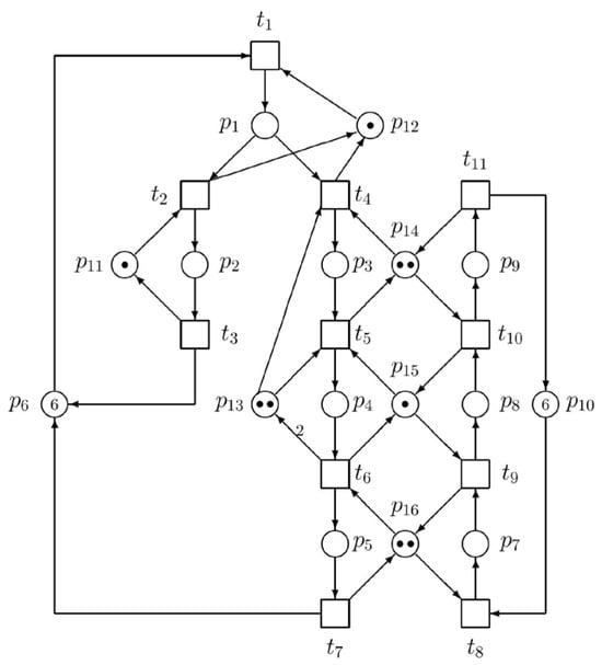
Figure 1.
The GPN model of AMS, where W(t6,p13) = 2.
Clearly, not only the structure but also the structural properties of ES3PR (reachability tree/graph, invariants, siphons, etc.) are different from those of S3PR. Consequently, siphon-based procedures of finding the supervisor, ensuring deadlock-freeness of the final system controlled by this supervisor, have to be different.
The set M expressing states of marking of particular PN places, simply said the PN marking M, is an (n × 1) vector also named the state vector. Its evolution is performed by means of the matrix/vector equation Mk+1 = Mk + [N]. σk, k ∈ ℕ, where M0 is an initial marking. This equation represents the mathematical model of the net N. The matrix [N] = [Post]T − [Pre] is the (n × m) incidence matrix. It represents the matrix notation of the set F. It can also be expressed as [N] (p, t) = W (t, p) − W (p, t). After all, σk is an (m × 1) vector expressing the firing of transitions also named the control vector. Namely, it expresses the state of transitions (a transition is able to be fired (i.e., it is enabled))—it is indicated by 1, or not—it is indicated by 0. If a transition is enabled, it may or may not be fired.
For a place p, M(p) is an integer indicating the number of tokens placed inside of this place. We say that the place p is marked by M iff M(p) > 0. The abbreviation iff means in the whole paper if and only if.
A subset D ⊆ P is marked by M iff at least one place p ∈ D is marked by M. Thus, M(D) = Σp ∈ D M (p) denotes the sum of tokens in all places in D.
●x = {y ∈ P ∪ T | (y, x) ∈ F} is the preset of a node x ∈ P ∪ T, while x● = {y ∈ P ∪ T | (x, y) ∈ F} is the postset of a node x ∈ P ∪ T.
A transition t such that |t●| > 1 is named a fork. A transition t such that |●t| > 1 is named a join. A place p such that |p●| > 1 is named a choice. A place p such that |●p| > 1 is named an attribution.
SP (x1, xn) means a simple path from x1 to xn. It is a path whose nodes are all different.
We say that a transition t ∈ T is enabled at a marking M iff ∀p ∈ ●t, M(p) ≥ W (p, t). After firing t, a new marking M′ is evolved such that ∀p ∈ P, M′ (p) = M(p) − W (p, t) + W (t. p). However, enabled transition t may be fired, but it also may not be fired.
A non-empty subset of places S ⊆ P is a siphon iff ●S ⊆ S●. A non-empty subset of places S ⊆ P is a trap iff S● ⊆ ●S. Siphon S is minimal iff it contains no other siphons (as its proper subset). If a minimal siphon S does not contain a marked trap, it is named strict.
There are many approaches to computing the siphons of Petri nets. Let us introduce some of them:
- Using the sign incidence matrix—see [2];
- Using the incidence matrix in an evolutionary algorithm [3];
- Using problem partitioning [4];
- Using the tensor product of matrices [5];
- Based on place constraints [6];
- Using condition for a resource subset [7];
- Using mixed-integer programming [8];
- And many others.
Such approaches offer algorithms but not tools for users applying siphons in solutions to other problems. For the user, it is a more useful tool in which the structural parameters of a Petri net create an input and the tool directly offers corresponding siphons. Moreover, these tools yield the possibility of drawing Petri nets and graphical inputs/outputs in the testing of their properties and performing some other applications. Such tools are, e.g.,
- (i)
- The Petri net toolbox for the system MATLAB (but it does not belong to the MATLAB 6 standard fittings and it must be paid for);
- (ii)
- The toolbox GPenSim, which is free.
Accordingly, the latter tool was preferred in this paper.
A column vector I: P → Z indexed by P, where Z is the set of integers, is named the P-vector. A column vector J: T → Z indexed by T is named the T-vector. For the economy of space, a P-vector I is denoted by Σp∈ P I (p)p and T-vector J is denoted by Σt ∈ T J(t)t.
Let I be a P-invariant of (N, M0). Then, ∀M ∈ R (N, M0), IT.M = IT.M0. Here, R (N, M0) is the state space of N. In other words, it is a set of all reachable markings of N.
The state enumeration methods compute the reachability tree (RT). The nodes of RT represent the Petri net states corresponding to a given initial state. For different initial states, the corresponding RTs are different. In our paper, we do not use RT (i.e., reachability graph (RG), because when we connect the nodes of RT with the same name into a single node, we obtain RG) for computing the supervisor structure. We use siphons for the supervisor synthesis. There exist methods for the supervisor synthesis based on RT—see, e.g., the paper [9], where its comparison with a siphon-based approach for S3PR is introduced.
Regarding data inhibitor arc methods, there exist works such as [10,11,12]. However, due to the use of data inhibitor arcs, the controlled net is no longer a Petri net in the common sense.
As we can see, the invariant I is a P-vector. ||I|| = {p ∈ P | I(p) ≠ 0} means a support of P. ||I||+ = {p ∈ P | I(p) > 0} is the positive support of P and ||I||− = {p ∈ P | I(p) < 0} is the negative support of P.
P-invariant of (N, M0) is a natural solution of the equation IT. [N] = 0. If all elements of P-invariant I are non-negative, this invariant is named P-semiflow.
T-invariant of (N, M0) is a natural solution of the equation [N]. J = 0. It gives information about a possible loop in the net, i.e., about a sequence of transitions that leads back to the marking it starts in. If all elements of T-invariant J are non-negative, this invariant is named T-semiflow.
When a place p is given, then max t ∈ p● {W (p, t)} is denoted by maxp●.
More details about PN are introduced in [1,13,14,15] and in basic papers about PN [16,17,18,19].
1.2. Structure of the Article
In the next section, preliminaries concerning definitions of particular PN models of AMS are introduced.
The Section 3 is devoted to the control of the ES3PR paradigm of the AMS model. It represents one of the two substantive parts of this paper. Since the ES3PR model belongs to a subclass of the S4P paradigm of models, such a paradigm is defined there. The basic influence of siphons on the control of PN models of AMS is emphasized there too. Finally, definitions concerning the siphon-based control and procedure make it possible to ensure that the parameters of the supervisor, which ensure the deadlock-freeness of the ES3PR model, are introduced. To illustrate the ES3PR model, a simple example is presented in Figure 1 and its siphons are computed. Unfortunately, these siphons that satisfy S3PR models cannot be used for the supervisor synthesis of the ES3PR model. Namely, they do not ensure the deadlock-freeness.
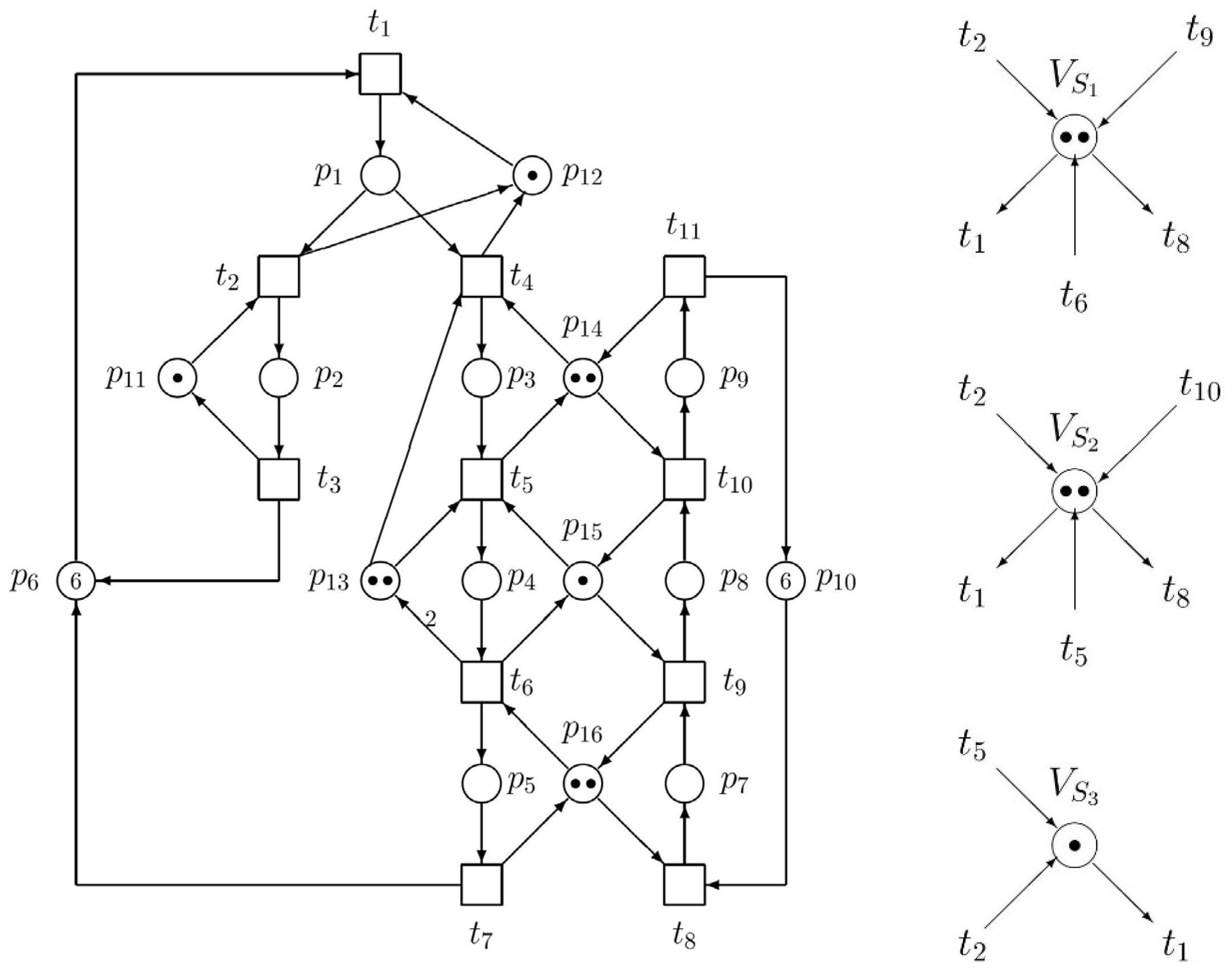
In the Section 4, representing the second of two substantive parts of the paper, the controllability of siphons in GPN is analyzed, and elementary and dependent siphons are checked regarding the max cs property. Then, the supervisor computed in the sense of such a procedure is set. Figure 2 illustrates the interconnections between the original uncontrolled model and the supervisor ensuring the deadlock-freeness of the controlled object.

Figure 2.
The ES3PR paradigm of the original GPN model of AMS (left) and the supervisor (right) consisting of three monitors.
The Section 5 concerns further research.
The Section 6 constitutes the conclusions, where the topic and contribution of the paper are evaluated and further work for the future is highlighted.
2. Preliminaries
As for the nomenclature of sets in PN used below, PS is a set of operation places, PR is a set of resource places, and P0 is a set of idle places.
Definition 1 ([20]).
An ordinary Petri net N = (PS ∪ {p0}, T, F) is a simple sequential process (S2P) when the following hold true:
- 1.
- PS ≠ ∅, p0 ∉ PS.
- 2.
- N is a strongly connected state machine (i.e., OPN, where each transition has only one input place and only one output place).
- 3.
- Every circuit in N contains place p0.
Definition 2 ([20]).
An extended simple sequential process with resources—ES2PR—is a generalized pure Petri net N = (PS ∪ {p0} ∪ PR, T, F, W), such that:
- 1.
- The subnet generated by the set X = PS ∪ {p0} × T is an S2P.
- 2.
- PR ≠ ∅ and (PS ∪ {p0}) ∩ PR = ∅.
- 3.
- ∀t ∈ T, ∀p ∈ ●t, W (p, t) = 1.
- 4.
- ∀r ∈ PR, ∃ a minimal P-semiflow Ir such that {r} = ||Ir|| ∩ PR, p0 ∉ ||Ir||, ||Ir|| ∩ PS ≠ ∅ and Ir(r) = 1.
Definition 3 ([20]).
Let N = (PS ∪ {p0} ∪ PR, T, F, W) be an ES2PR. An initial marking M0 is acceptable for N iff:
- 1.
- M0(p0) > 0.
- 2.
- ∀p ∈ PS, M0(p) = 0.
- 3.
- ∀r ∈ PR, M0(r) > 0
- 4.
- Elements in the support of each minimal T-semiflow can be fired sequentially
Definition 4 ([20]).
An ES3PR is the composition of a finite set of ES2PR via the fusion of resource places.
Definition 5 ([20]).
Let Ni = (Pi, Ti, Fi, Wi) (i = 1, 2) be two generalized Petri nets. Then:
- 1.
- N1 and N2 are composable (via fusion of places) iff T1 ∩ T2 = ∅, and PC = P1 ∩ P2 ≠ ∅.
- 2.
- Net N = (P, T, F, W) is called the composed net of N1 and N2, denoted by N1 ○ N2, where P = P1 ∪ P2, T = T1 ∪ T2, W (p, t) = if t ∈ T1 then W1 (p, t) else W2 (p, t).
Definition 6 ([20]).
Let Im be a set of indices and Ni = (Pi, Ti, Fi, Wi) (i ∈ Im) be a set of generalized Petri nets. We denote by N = ◯i ∈ Im Ni the net obtained by the following operation: if card (Im) = 1, then N = N1; else, N = Nk ○ ◯ i ∈ Im \ {k} Ni.
Definition 7 ([20]).
An ES3PR is the composition of a finite set of ES2PR via the fusion of resource places.
Definition 8 ([20]).
(N, M0), ◯i ∈ Im Ni, Ni= (Pi, Ti, Fi, Wi), and (Ni, M0i) being initially acceptably marked ES2PR, is an acceptably marked ES3PR iff:
- 1.
- ∀i ∈ Im, ∀p ∈ PSi ∪ {p0i}, M0(p) = M0i (p).
- 2.
- ∀i ∈ Im, ∀r ∈ PR, M0(r) = if card (Im) = 1 then M0i(r) else maxi ∈ Im M0i(r).
In [21], the following property was proved:
Let N = (PS ∪ P0 ∪ P, T, F, W) be an ES3PR, where P0 = ∪i ∈ Im {p0i}. Then, rank ([N]) = |PS|.
In [22], the following Theorem was proved:
Theorem 1 ([22]).
Let S be a strict minimal siphon in an ES3PR N = (PS ∪ P0 ∪ P, T, F, W). Then, S = SR ∪ SS satisfies S ∩ P0 = ∅, S ∩ PR = SR ≠ ∅, and S ∩ PS = SS ≠ ∅.
3. Control of ES3PR
The paradigm ES3PR models a class of concurrently cyclic sequential processes sharing common resources. An approach to deadlock prevention by controlling siphons in ES3PR will be presented here. Namely:
- The control of elementary siphons;
- Finding the relevant approach to finding conditions for control of dependent siphons;
- Finding a way to make the ES3PR deadlock-free.
With respect to [20], ES3PR is a subclass of S4R (Systems of Sequential Systems with Shared Resources) defined by the next definition.
Definition 9 ([20]).
An S4R is a generalized pure net N = ◯i ∈ Im Ni = (P, T, F, W), where
- 1.
- Ni = (PSi ∪ {p0i} ∪ PRi, Ti, Fi, Wi), i ∈ Im.
- 2.
- P = Ps ∪ P0 ∪ PR is a partition such that:
- PS = ∪ i ∈ Im PSi, PSi ≠ ∅ and PSi ∩ PSj = ∅, ∀i ≠ j (i, j ∈ Im);
- PR = ∪ i ∈ Im PRi = {r1, r2, …, rn}, n > 0;
- P0 = ∪ i ∈ Im {p0i};
- The elements in P0, PS, and PR are called idle, operation, and resource places, respectively;
- The output transitions of an idle place are called source transitions.
- 3.
- T = ∪ i ∈ Im Ti, Ti ≠ ∅, Ti ∩ Tj = ∅ for all i ≠ j.
- 4.
- ∀i ∈ Im the subset Ni generated by PSi ∪ {p0i} ∪ Ti is a strongly connected state machine such that every cycle contains p0i.
- 5.
- ∀r ∈ PR, there exists a unique minimal P-semiflow Ir ∈ IN|P| (here IN = {0, 1, 2, …}) such that {r} = ||Ir|| ∩ PR, P0 ∩ ||Ir|| = ∅, PS ∩ ||Ir|| ≠ ∅ and Ir(r) = 1.
- 6.
- PS = ∪ r ∈ PR (||Ir||\{r}).
- 7.
- N is a strongly connected net.
S4PR is still more complicated than S4P. The complete definition of S4PR can be found, e.g., in [23,24] and in several others.
In [22], the following theorem was proved:
Theorem 2 ([22]).
Let (N, M0) be a marked S4R net. N is live under M0 iff it satisfies the max cs property.
Consider that r is a resource place, S is a strict minimal siphon and H(r) = Ir\{r} in a S4R net. We can define Th(S) = Σr∈ SR H (r)\S. It can be seen that |Th(S)| ⊆ PS is true. Use Σp∈ |Th(S)| hS(p)p to denote Th(S). hS(p) indicates that if the number of tokens in p increases by one, the siphon S loses hS (p) tokens
In [25], the following lemma was proved:
Lemma 1 ([25]).
Let (N, M0) be a marked net and S be a siphon of N. S is max-controlled if there exists a P-invariant I such that ∀p ∈ (||I||- ∩ S), maxp● = 1, ||I||+ ⊆ S, and Σp ∈ P I (p)M0(p) > Σp ∈ S I(p) (maxp● − 1).
This lemma will be applied below within the context of Figure 2.
3.1. Siphons in Petri Nets Control
Siphons and traps were formally defined above at the end of the introduction. Elementary and dependent siphons in OPN were proposed in [26]. Later, the terminology was more specified in [27]. In this section, siphons and traps are defined in GPN.
With respect to [28], we have the following knowledge:
Definition 10 ([28]).
Let S⊆ P be a subset of places of N = (P, T, F, W). P-vector λS is called the characteristic P-vector of S iff∀p∈ S, λS(p) = 1; otherwise λS(p) = 0.
Definition 11 ([28]).
Let S⊆ P be a subset of places of N = (P, T, F, W). ηS is called the characteristic T-vector of S iff ηTS = λTS.[N].
Definition 12 ([28]).
Let N = (P, T, F, W) be a net with |P| = n, which has k siphons S1, …, Sk, m, k∈ ℕ+. We define [λ]k×n = [λS1|λS2|… |λSk]T and [η]k×m = [λ]k×n.[N]n×m = [ηS1|ηS2||…|ηSk]T is called the characteristic matrix of the siphons in N.
Definition 13 ([28]).
Let ηSα, ηSβ, …, and ηSγ ({α, β, …, γ}⊆{1, 2, …, k}) be a linearly independent maximal set of the matrix [η]. Then, ΠE = {Sα, Sβ, …, Sγ} is called a set of elementary siphons in N.
Definition 14 ([28]).
S∉ ΠE is called a strongly dependent siphon if ηs =ΣS∈ ΠE ai.ηsi, where ai ≥ 0.
Definition 15 ([28]).
S∉ ΠE is called a weakly dependent siphon if∃ non-empty A, B ⸦ ΠE, such that A ∩ B =∅ and ηS =Σ Si∈A ai.ηSi −ΣSi∈ B ai.ηSi, where ai > 0.
Lemma 2 ([28]).
The number of elements in any set of elementary siphons in net N equals the rank ([η]).
Verbally said, this important lemma shows that the rank ([η]) directly determines the number of elementary siphons. However, it simultaneously determines also the number of dependent siphons because Π = ΠE ∪ ΠD.
Theorem 3 ([28]).
Let NES be the number of elementary siphons in net N = (P, T, F, W). Then, NES ≤ min {|P|, |T|}.
Corollary 1 ([28]).
Let N =◯i∈ Im Ni, Ni= (Pi, Ti, Fi, Wi) be an ES3PR. Then, NES ≤ |PS|.
Verbally said, this important corollary indicates that the maximal number of elementary siphons in an ES3PR net is not greater than the number of its operation places p ∈ PS.
3.2. Procedure of Setting the Supervisor for ES3PR
In [20,28], the following definition can be found:
Definition 16 ([20,28,29]).
Let S be a strict minimal siphon in an ES3PR net model of a plant (Nµ0, Mµ0), where Nµ0 = ◯i ∈ {1, …, n} Ni = (P0 ∪ PS ∪ PR, T, Fµ0, Wµ0). Let {α, β, …, γ} ⊆ {1, 2, …, n} such that i ∈ {α, β, …, γ}, |ThS| ∩ p ∈ PSi ≠ ∅ and ∀j ∈ {1, 2, …, n} \ {α, β, …, γ}, |ThS| ∩ p ∈ PSj ≠ ∅. For S, a non-negative P-vector kS is constructed as follows:
- Step 1:
- ∀p ∈ P0 ∪ PS ∪ PR, kS(p): = 0;
- Step 2:
- ∀p ∈ |Th(S)|, kS(p): = hS(p), where Th(S) = Σp∈|Th(S)| hS(p)p;
- Step 3:
- ∀i ∈ {α, β, …, γ}, let ps ∈ ||ThS|| ∩ PSi be such a place that ∀pt ∈ SP (pu, p0i), pu ∈ ps••, pt ∉ |T h(S)|. Suppose that there are m such places p1s, p2s, …, pms. Assuredly, we have {pis |i = 1, 2, …, m} ⊆ |Th(S)| ∩ PSi. ∀pis let piν ∈ SP (p0i, pis) be such a place that hS(piν) > hS(pw), ∀pw ∈ SP (p0i, pis). ∀px ∈ SP (p0i, pis), kS(px): = hS(piν).
- Step 4:
- ∀Im’ ⊆ {1, 2, …, m}. ∀py ∈ ∩ i ∈ Im’ SP (p0i, pis), kS(py): = hS(piz), where piz ∈ |Th(S)| ∩ PSi, and ∄p ∈ Th(S) ∩ PSi, s.t. hS(p) > hS(piz).
In general, such a procedure makes it possible to finalize the supervisor synthesis, especially to set markings of the supervisor monitors VSi, i = 1, 2, …
3.3. Illustrative Example of ES3PR—Siphons and P-Invariants
Let us apply the theory of siphon-based control, introduced above, as an example of ES3PR. Consider the GPN in Figure 1 for modelling an AMS. Here, the set of operation places is PS = {p1, p2, p3, p4, p5, p7, p8, p9}, the set of resource places is PR = {p11, p12, p13, p14, p15, p16}, and the set of idle places is P0 = {p6, p10}.
As we can see in Figure 1, there exists one arc with a weight equal to 2—notice the arc from t6 to p13. Consequently, the GPN is shown in Figure 1. The state space of the net N expressed by the reachability tree (RT) has 308 nodes (including the initial state). Because of such a large number of nodes, the RT cannot be displayed here. The minimal siphons are introduced in Table 1.

Table 1.
Siphons and traps of the PN model.
The Petri net in Figure 1 models a general real manufacturing system. In its essence, this model, based on a generalized Petri net, models a real production system consisting of three machine tools and three robots. Robots serve machine tools at the input as well as at the output. The manufacturing system consists of three cooperating subsystems—three cooperating production processes, namely {t1, p1, t2, p2, p12, t3, p6, p11, t1}, {t1, p1, t4, p12, p3, t5, p14, p4, t6, p13, p15, p5, p16, t7, p6, t1} and {t8, p7, t9, p16, p8, t10, p15, p9, t11, t14, p10, t8}. They produce three kinds of parts. Consequently, there are three machines M1–M3 (represented by places p14, p15, p11). There are also three robots R1–R3 (represented by places {p12, p16, p13}) feeding parts/material into machines or taking it out of them. There is the directed arc from t6 to p13 with a weight of 2. This means that the corresponding device is able to work with two parts simultaneously. Thus, {p6, p10} are idle places, {p11–p16} are resources and the rest of the places represent operation places. Operation places formally represent operations in progress in corresponding devices (i.e., in resource places executing them).
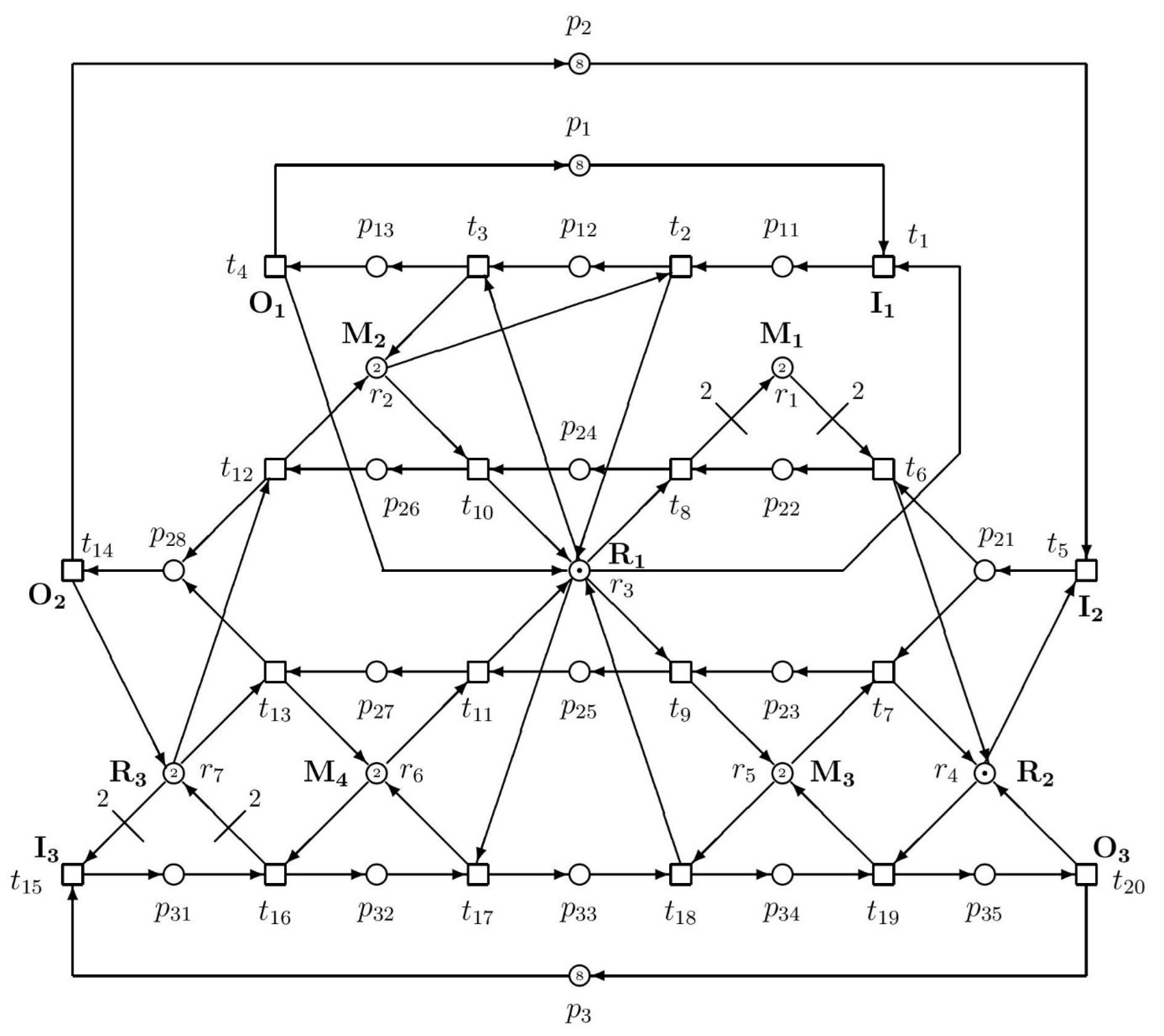
In the future, we will examine larger systems (e.g., like that in Figure 3).

Figure 3.
A larger ES3PR paradigm with industrial application, where M1–M4 are machines, R1–R3 are robots, I1–I3 are inputs of raw materials and/or semi-products, and O1–O3 are outputs of produced final parts.
As we can see in Table 1, there exist 11 minimal siphons in this GPN model of AMS. They can be enumerated, e.g., by the tool GPenSIM [30,31,32] or by other PN tools. Because the traps corresponding to the crossed siphons are marked, crossed siphons may be omitted from the list of siphons. Hence, only four of the siphons are strict minimal siphons—S3, S7, S8 and S10. The other seven siphons are not relevant because they are equal to corresponding traps.
Let us renumber siphons S3, S7, S8 and S10 into siphons S3, S1, S2 and S4, respectively. Consequently, S1 = {p5, p8, p15, p16}, S2 = {p4, p9, p14, p15}, S3 = {p4, p13} and S4 = {p5, p9, p14, p15, p16}. In the form of row P-vectors, they are as follows:
- S1 = (0, 0, 0, 0, 1, 0, 0, 1, 0, 0, 0, 0, 0, 0, 1, 1)
- S2 = (0, 0, 0, 1, 0, 0, 0, 0, 1, 0, 0, 0, 0, 1, 1, 0)
- S3 = (0, 0, 0, 1, 0, 0, 0, 0, 0, 0, 0, 0, 1, 0, 0, 0)
- S4 = (0, 0, 0, 0, 1, 0, 0, 0, 1, 0, 0, 0, 0, 1, 1, 1)
The corresponding matrix [λ] = [S1T, S2T, S3T, S4T]T can be utilized (analogically to [1] in the case of the S3PR paradigm) for finding potential interconnections with the supervisor eliminating the deadlocks. Namely, when we multiply matrix [λ] by [N], which is the (16 × 11) dimensional incidence matrix of GPN in Figure 1, we obtain the matrix [η] = [λ]. [N] = [η1T, η2T, η3T, η4T]T consisting of the following T-vectors
- η1 = (0, 0, 0, 0, −1, 1, 0, −1, 1, 0, 0)
- η2 = (0, 0, 0, −1, 1, 0, 0, 0, −1, 1, 0)
- η3 = (0, 0, 0, −1, 0, 1, 0, 0, 0, 0, 0)
- η4 = (0, 0, 0, −1, 0, 1, 0, −1, 0, 1, 0).
Hence, we have λS1 = p5 + p8 + p15 + p16, λS2 = p4 + p9 + p14 + p15, λS3 = p4 + p13, λS4 = p5 + p9 + p14 + p15 + p16 and ηS1 = −t5 + t6 − t8 + t9, ηS2 = −t4 + t5 − t9 + t10, ηS3 = −t4 + t6, and ηS4 = −t4 + t6 − t8 + t10. It is easy to verify that ηS4 = ηS1 + ηS2. However, this set of vectors ηSi, i = 1, …, 4 is not linearly independent, because η4 = η1 + η2, i.e., rank([η]) = 3, and rank([η]) = NES = 3 < rank([N]) = 8. It means that there are three elementary siphons and one strongly dependent siphon. Thus, ΠE = {S1, S2, S3} and ΠD = {S4}.
In Figure 1, we have p01 = p6, p02 = p10, PS1 = {p1, …, p5}, PS2 = {p7, …, p9}, PR1 = {p11, …, p16}, and PR2 = {p14, …, p16}. Unfortunately, the system is deadlocked, i.e., not live.
The GPN in Figure 1 has eight minimal P-invariants (see Table 2). They may also be computed, e.g., by PN tools [30,31,32]. Namely, I1 = p2 + p11, I2 = p1 + p12, I3 = p3 + 2p4 + p13, I4 = p3 + p9 + p14, I5 = p4 + p8 + p15, I6 = p5 + p7 + p16, I7 = p1 + p2 + p3 + p4 + p5 + p6 and I8 = p7 + p8 + p9 + p10. In Table 2, we can see P-invariants in the form of row vectors. Negative elements in the vectors ηi in the S3PR paradigm (see [1]) mean that directed arcs are emerging from the GPN model and enter through corresponding transition ti (index i depends on the position of the transition in a vector ηj) to the supervisor, while positive elements represent directed arcs in opposite direction, i.e., from the supervisor to the GPN model through corresponding transitions. However, in the case of ES3PR, as well as S4P paradigms, the supervisor synthesis is not as simple as in the S3PR paradigm. The structural properties presented here will be applied in the continuation of this example introduced in Section 4.3.
Table 2.
P-invariants in the form of row vectors.
If we applied these parameters (which are suitable for S3PR) to ES3PR, we would find that the responding supervisor does not comply with such a paradigm of the AMS model because it does not prevent deadlocks.
4. Controllability of Siphons in Generalized Petri Nets
The deadlock prevention policy for GPN consists of the request that all siphons (elementary as well as dependent) must satisfy maximal cs property. The elementary siphons in the GPN model are properly supervised by means of explicitly adding monitors for them with appropriate initial markings.
Therefore, the controllability of both the elementary siphons and the dependent ones will be analyzed. For the siphon control, the facts from Section 3.1 will be utilized.
In [25,33], the following three important definitions are introduced:
Definition 17 ([25,33]).
Let the net (N, M0) be a marked net and S be a siphon of N. S is said to be max-marked (min-marked) at a marking M iff ∃p ∈ S such that M(p) ≥ maxp• (M(p) ≥ minp•);
Definition 18 ([25,33]).
Let the net (N, M0) be a marked net and S be a siphon of N. S is said to be max-controlled iff S is max-marked at any reachable marking;
Definition 19 ([25,33]).
A net (N, M0) is said to be satisfying the max cs property (controlled-siphon property) iff each minimal siphon of N is max-controlled.
Thus, in our case (see Example in Section 4.2), we have four strict minimal siphons. All of them have to be max-controlled. Each siphon satisfying the cs property can be always sufficiently marked. Consequently, it can allow firing a transition at least once.
Namely, in [33], the following lemma is proved:
Lemma 3 ([25,33]).
If a net (N, M0) satisfies the max cs property, it is deadlock-free.
As was explained above, strict minimal siphons in an ES3PR consist of both elementary siphons and dependent ones. Monitors are explicitly added only to the elementary siphons. However, so that they satisfy the max cs property, the question arises as to how to ensure the max cs property in the case of dependent siphons. This is ensured by means of the max cs property of elementary siphons. Namely, this is performed by properly selecting the control depth variables ξSi of its elementary siphons Si. Below, in Section 4.1 and Section 4.2, results relevant not only to the controllability of elementary siphons but also to the controllability of dependent siphons are presented as well.
4.1. Controllability of Elementary Siphons
Here, for elementary siphon control, the knowledge from Section 3.1 especially will be utilized. Moreover, the following definition for setting the markings to monitor VSi creating the supervisor will be applied.
Definition 20 ([20]).
Let S be a strict minimal siphon in an ES3PR model (Nμ0, Mμ0), where N = ◯i∈ {1.,…, n} Ni = (P0 ∪ PS ∪ PR, T, Fμ0,Wμ0). Let {α, β, …, γ} ⊆ {1,2, …, n} such that ∀i ∈ {α, β, …, γ}, |Th(S)| ∩ PSi ≠ ∅ and ∀j ∈ {1, 2, …, n} \ {α, β, …, γ}, |Th(S)| ∩ PSj ≠ ∅. For S, a non-negative P-vector kS is constructed in four steps introduced above in Definition 16.
Almost every fact introduced below in Section 4.2 touches on both elementary siphons and dependent ones.
4.2. Controllability of Dependent Siphons
In addition to the control of elementary siphons, the control of dependent siphons is also very important.
Lemma 4 ([33]).
Let (N, M0) be a marked net and S be a siphon of N. S is max-controlled if there exists a P-invariant I such that ∀p ∈ (||I||− ∩ S), maxp• = 1, ||I||+ ⊆ S, and Σp ∈ P I(p)M0(p) > Σp∈S I(p) (maxp• − 1).
When in an S4R net r is a resource place, S is a strict minimal siphon and H(r) = Ir\{r}. Let Th(S) = Σr∈ SR H(r)\S. We can see that |Th(S)| ⊆ PS is true. Let us use Σp∈|Th(s)| hS(p)p to denote Th(S). With respect to Theorem 2 at the beginning of Section 3, hS(p) shows that siphon S loses just hS(p) tokens if the number of tokens in p increases by one.
In [20], the following theorem (such a theorem is also introduced in [28]) dealing with strongly dependent siphons is introduced:
Theorem 4 ([20,28]).
Let (N, M0), N = (P, T, F, W) be a marked net and S be a strongly dependent siphon with ηS = Σi∈ {1, n} aiηSi, where S1, …, Sn are elementary siphons of S. S is max-controlled if
- 1.
- ∀i ∈ {1, 2, …, n}, Ii is a P-invariant of N, ||Ii||+ = Si, and ∀p ∈ Si, Ii(p) = 1;
- 2.
- M0(S) > Σi∈ {1, n}Σp∈||Ii||− (ai|Ii(p)|M0(p)) + Σp∈ S (maxp• − 1).
In Example 3.3 of ES3PR, the siphon S4 = {p5, p9, p14, p15, p16} is, due to ηS4 = ηS1 + ηS2, a strongly dependent siphon, and S1 and S2 are its elementary siphons. Using the previous Theorem 4, we can verify the controllability of S4. As for Figure 2, h1 and h2 are P-invariants, satisfying condition 1 of Theorem 4. Now, we only have to check condition 2 of Theorem 4: Σi∈ {1, 2} Σp∈||hi||− (ai|hi(p)|Mµ1(p)) + Σp∈S4 (maxp• − 1). After computing the supervisor consisting of monitors VSi, i = 1, …, 3, we may denote the controlled net as (Nµ1, Mµ1).
4.3. Illustrative Example of ES3PR—Control
Let us continue with the illustrative example introduced in Section 3.3. While there, the GPN model and its structural properties were presented, here, supervisor synthesis will be performed.
In our example of ES3PR, we have P0 = {p6, p10}, where p01 = p6, p02 = p10, PS1 = {p1, …, p5}, PS2 = {p7, …, p9}, PR1 = {p11, …, p16}, PR2 = {p14, …, p16}.
Ip15 = p4 + p8 + p15 and Ip16 = p5 + p7 + p16 are minimal P-semiflows associated with resource places p15, p16, respectively. Hence, Th(S1) = (H(p15) + H(p16))\S1 = ((p4 + p8) + (p5 + p7))\{p5, p8} = p4 + p7. Ip14 = p3 + p9 + p14 and Ip15 = p4 + p8 + p15 are minimal P-semiflows associated with resource places p14, p15, respectively. Hence, Th(S2) Σp ∈ P h2(p)Mµ1 (p) = Mµ1 (p14) + Mµ1 (p15) − Mµ1 (VS2) = 2 + 1 − 2 = 1 > Σp ∈ S2 h2(p) (maxp• − 1) = 0. Thus, we can say that S2 is max-controlled by P-invariant h2.
P-invariants hi, i = 1, 2, and 3 indicate how the structure of interconnections of monitors VSi (in Figure 2 right) with the net model representing the original uncontrolled plant will look. Marking of particular monitors VSi needs to be computed as can be seen below: h1 and h2 are P-invariants satisfying condition 1 of the above-introduced Theorem 4.
To check condition 2 of Theorem 4, Σi∈ (1,n) Σp∈ ||hi||− (ai|hi(p)|Mµ1(p)) + Σp ∈ S4 (maxp• −1) = Mµ1(p1) + Mµ1(p3) + Mµ1(p7) + Mµ1(VS1) + Mµ1(VS2) + (1−1) = (0 + 0 + 0 + 2 + 2 + 0) = 4. Meanwhile, Mµ1(S4) = Mµ1(p14) + Mµ1(p15) + Mµ1(p16) = 5. Thus, S4 is max-controlled. When we consider VS1, VS2 we see that based on them we have Σi∈ (1,2)Σp∈ ||hi||− (ai|hi(p)|Mµ1 (p)) + Σp∈ S4 (maxp• −1) = Mµ1(p1) + Mµ1(p3) + Mµ1(p7) + Mµ1(VS1) + Mµ1(VS2) + (1−1) = (0 + 0 + 0 + 2 + 2 + 0) = 4. Meanwhile, Mµ1(S4) = Mµ0(S4) = Mµ1(p14) + Mµ1 (p15) + Mµ1 (p16) = 5. Thus, S4 is max-controlled. Because gS = kS + Vs is a P-invariant of the resultant net system (Nµ1, Mµ1), a monitor Vs is added to the original net model (Nµ0, Mµ0). Thus, Nµ1 = (P0 ∪ PS ∪ PR ∪ VS, T, Fµ1, Wµ1), ∀p ∈ P0 ∪ PS ∪ PR, Mµ1(p) = Mµ0(p). Let hS = Σr∈SR Ir − gS and Nµ1(VS) = Mµ0(S) − ξS (ξS ∈ ℕ). Then, S is max-controlled if ξS > Σp∈ S hS(p) (maxp• − 1).
As we can see in Figure 2, (Nµ0, Mµ0) is an ES3PR, which is the model of plant net, and (Nµ1, Mµ1) is its liveness-enforcing supervisor. Monitors are added to control elementary siphons S1 − S3 only. They enforce liveness for (Nµ0, Mµ0).
The number NES of elementary siphons is bounded—see Theorem 3 in Section 3.1 (it is smaller than the minimum of the pair the place count and the transition count). Therefore, dependent siphons have to be implicitly controlled by fittingly setting the initial number of tokens in monitors. Thus, we can obtain a structurally simple liveness-enforcing PN supervisor for an ES3PR paradigm of the plant net model.
In Figure 1 we have PS1 = {p1, …, p5}, PS2 = {p7, …, p9}. For S1 = {p5, p8, p15, p16} we have Th(S1) = p4 + p7. With respect to the procedure described in Section 3.1: For PS1 we have p1s = p4, p1ν = p4, p1z = p4. For PS2 we have p2s = p2ν = p2z = 7. Finally, kS1 (p1) = kS1 (p3) = kS1 (p4) = kS1 (p7) = 1. ∀p ∈ PS \ {p1, p3, p4, p7}, kS1 (p) = 0. Naturally, we obtain kS1 (p6) = kS1(p10) = kS1 (p11) = kS1(p12) = kS1(p13) = kS1(p14) = kS1 (p15) = kS1 (p16) = 0 since p6 and p10 are idle places and p11, …, p16 are resource places. Let KS = {p | kS (p) ≠ 0, p ∉ |Th(S)|}. In Figure 1 we have KS1 = {p1, p3}.
In Figure 2, we have the following results:
- g1 = p1 + p3 + p4 + p7 + VS1 and l1 = Ip15 + Ip16 = p4 + p8 + p15 + p5 + p7 + p16 are P-semiflows. Let h1 = l1 − g1. h1 = p5 + p8 + p15 + p16 − p1 − p3 − VS1 is a P-invariant. When we notice that ||h1||− ∩ S1 = ∅, ||h1||+ = S1, and Σp∈ P h1(p)Mµ1 (p) = Mµ1 (p15) + Mµ1 (p16) − Mµ1 (VS1) = 1 + 2 − 2 = 1 > Σp∈ S1 h1(p) (maxp• − 1) = 0 we can say that S1 is max-controlled by P-invariant h1.
- g2 = p1 + p3 + p7 + p8 + VS2 and l2 = Ip14 + Ip15 = p3 + p9 + p14 + p4 + p8 + p15 are P-semiflows of the controlled net. Let h2 = l2 − g2. h2 = p4 + p9 + p14 + p15 − p1 − p7 − VS2 is hence a P-invariant. When we notice that ||h2||− ∩ S2 = ∅, ||h2||+ = S2, and Σp∈ P h2(p) Mµ1(p) == Mµ1 (p14) + Mµ1 (p15) − Mµ1 (VS1) = 2 + 1 − 2 = 1 > Σp ∈ S2 h1(p) (maxp• − 1) = 0, we can say that S2 is max-controlled by P-invariant h2.
- g3 = p1 + p3 + VS3 and l3 = Ip13 = p3 + p4 + p13 are P-semiflows. Let h3 = l3 − g3. h3 = p4 + p13 − p1 − VS3 is a P-invariant. When we notice that ||h3||− ∩ S3 = ∅, ||h3||+ = S3 and Σp∈ P h3(p)Mµ1 (p) = Mµ1(p16) − Mµ1 (VS3) = 2 − 1 = 1 > Σp∈ S3 h3(p) (maxp• − 1) = 0 which implies that S3 is max-controlled by P-invariant h3.
The supervised ES3PR is deadlock-free. To the left, the original GPN model of the plant is displayed, while to the right, its supervisor is placed. Both pictures are shown separately to avoid complicated and non-transparent interconnections between both the plant and the supervisor. Namely, their cooperation is stronger when one observes the insinuated transitions of the supervisor and corresponding real ones in the plant.
As we can see in Figure 2, 0 < ξS1 < 3, 0 < ξS2 < 3, 0 < ξS3 < 2, and ξS1 + ξS2 > 1. Let ξS1 = ξS2 = ξS3 = 1. Hence, we have Mµ1(VS1) = 2, Mµ1 (VS2) = 2, and Mµ1 (VS3) = 1. It is easy to verify that all strict minimal siphons are max-controlled—see results 1–3 introduced above in Section 3.3. Consequently, the net system in Figure 2 is live, i.e., deadlock-free.
4.4. Complexity Analysis
The most complex thing in the proposed method is the computation of siphons, especially in larger Petri net models with a great number of places and transitions and with intricate structures of interconnections (i.e., arcs) among them. There are many algorithms for computing siphons—see Section 1.1. We prefer the tool GPenSIM (see [30,31,32]), which offers not only computation of siphons but also invariants, reachability graphs, etc.
Besides the computation of siphons, in our procedure, we used some simple computations undemanding on time, based on linear algebra.
5. Future Work
In this paper, only a simple structure of the ES3PR paradigm of Petri net models of AMS was analyzed and its supervisor ensuring deadlock-freeness was synthesized by the siphon-based approach. In the future, we will aim at larger structures of ES3PR, e.g., that displayed in Figure 3.
Since information security—see [34,35]—is also very important for an automated manufacturing system, we will have to take this aspect into account as well.
6. Conclusions
Liveness (deadlock-freeness) is a very important property of PN from a behavioral point of view. Siphons, traps and invariants are structural objects of PN. Siphons especially are closely related to the PN liveness. There are many deadlock prevention control policies for AMSs (alternatively named flexible manufacturing systems—FMSs), based on siphons. Namely, AMSs are frequently modelled by PN-possessing siphons. There are many paradigms of PN models of AMS like S3PR, ES3PR, S4R, GS3PR, and many others.
To prevent deadlocks in AMS, liveness-enforcing supervisors are used. Most of the existing methods of their design are based on adding monitors (control places) for siphons. Monitors are based on exact controllability conditions for siphons. In this way, a liveness-enforcing supervisor with permissive behavior is obtained. However, as we have found, conditions of max controllability of siphons are overly restrictive and, in general, only sufficient.
The subject of this paper was to deal with the problem of deadlocks in the ES3PR paradigm of GPN models of AMS. This paper may be seen as a free continuation of the author’s paper [1], where a similar problem was resolved for the S3PR paradigm of ordinary PN (OPN) models of AMS. A difference between OPN and GPN consists of the weights of directed arcs. While in OPN, weights of directed arcs are only 1, in GPN, they may be greater than 1, i.e., multiplex arcs may occur. Therefore, the approach used in [1] to deal with deadlocks in S3PR is insufficient for dealing with deadlocks in ES3PR and it is necessary to find another one.
An empty siphon in an OPN can cause some transitions to be disabled forever. Therefore, it is necessary to prevent emptying siphons. Such a case in GPN is much more complicated. As a consequence of arcs with greater weights, an insufficiently marked siphon can lead to the occurrence of other deadlocks. Therefore, setting the marking of monitors VSi (which creates the supervisor) is very important, as is the selection of the control depth variables ξSi of elementary siphons Si.
ES3PN models of APN can be understood to be a subset of S4PR models, which are even much more complicated.
The approach presented here is based on verification of the max cs property of a net (N, M0). When such a net N satisfies this property, we can say that it is deadlock-free. In the case of GPN, a marked S4PR net is live if it satisfies the cs property. This means that the cs property is a sufficient but not necessary condition (unlike ES3PR) for the liveness of an S4R.
It was presented here that deadlock prevention in GPN models of AMS is much more complicated than that in OPN models of AMS. Simultaneously, the deadlock prevention of ES3PR (as a subclass of GPN models of AMS) was performed and illustrated as an example.
A more complex analysis of the deadlock prevention problem depends on specific paradigms of GPN. Namely, there are many paradigms of GPN with specific properties and corresponding specific policies for how to deal with deadlocks in them. For example, the specific paradigm GS3PR (generalized systems of simple sequential processes with resources) was analyzed in [36] as concerns the problem of deadlock prevention.
In the future, it will be necessary to be concerned with increasingly complicated structures of AMS modelled by GPN.
A serious review of siphon-based approaches to control GPN is presented in [37]. An application on a specific paradigm GS3PR was presented in [36].
Two ways of obtaining optimal supervisors are pointed out in the papers [38,39], where optimal supervisors are investigated, respectively, by means of linear monitors and by nonlinear constraints. As for an experimental comparison between our work and those related works, in order to show its advantages, it is necessary to say that our paper was motivated by the comparison of the deadlock prevention procedure for ES3PR presented here with that for S3PR presented in [1] and [9]. The ES3PR paradigm of the Petri net-based model of a manufacturing system must be built on GPN, while for the S3PR paradigm, the model built on OPN is sufficient.
Consequently, any other comparisons are a matter for our further research.
For the sake of completeness, it is necessary to say that we are interested here only in deadlock prevention. Namely, in general, there exist several distinguished understandings of procedures (independently of the Petri net) on how to provide systems against deadlocks—see [40]—namely deadlock prevention, deadlock detection and recovery, and deadlock avoiding. In our opinion, just deadlock detection and recovery [41] could be used in the case of attacks. But such approaches will have to be online.
It is necessary to say that siphon-based deadlock prevention is a static (i.e., offline) computational procedure consisting of finding the supervisor, which, after its application to the original plant with deadlocks, is able to ensure that the controlled plant will be deadlock-free, i.e., live (in the Petri net terminology).
In this paper, it was shown that the prevention of deadlocks in AMS with resources ensures a correct allocation of resources and thereby ensures the continuous and fluent operation of AMS. Thus, by means of controlling siphons of their PN-based models, the fluent and continuous operation of constituents in industrial production can be sustainable, which is very important in social practice.
Funding
This work was partially supported by the Slovak Grant Agency for Science VEGA under Grant No. 2/0020/21.
Data Availability Statement
Data is contained within the article.
Conflicts of Interest
The author declares no conflict of interest.
References
- Čapkovič, F. Petri Net Based S3PR Models of Automated Manufacturing Systems with Resources and Their Deadloc Prevention. Acta Polytech. Hung. 2023, 20, 79–96. [Google Scholar] [CrossRef]
- Boer, E.R.; Murata, T. Sign Incidence Matrix and Generation of Basis Siphons and Traps of Petri Nets. IEEE Trans. Circuits Syst. I Fundam. Theory Appl. 1994, 41, 266–271. [Google Scholar] [CrossRef]
- Tricas, F.; Colom, J.M.; Guervós, J.J.M. Using the incidence matrix in an evolutionary algorithm for computing minimal siphons in Petri net models. In Proceedings of the 18th International Conference on System Theory, Control and Computing ICSTCC, Sinaia, Romania, 17–19 October 2014; pp. 645–651. [Google Scholar] [CrossRef]
- You, D.; Karoui, O.; Wang, S.G. Computation of minimal siphons in Petri nets using problem partitioning approaches. IEEE/CAA J. Autom. Sin. 2022, 9, 329–338. [Google Scholar] [CrossRef]
- Han, X.; Chen, Z.; Liu, Z.; Zhang, Q. Calculation of siphons and minimal siphons in Petri nets based on semi-tensor product of matrices. IEEE Trans. Syst. Man Cybern. Syst. 2017, 47, 531–536. [Google Scholar] [CrossRef]
- Cordone, R.; Ferrarini, L.; Piroddi, L. Enumeration algorithms for minimal siphons in Petri nets based on place constraints. IEEE Trans. Syst. Man Cybern. A Syst. Hum. 2005, 35, 844–854. [Google Scholar] [CrossRef]
- Wang, S.; You, D.; Zhou, M. A necessary and sufficient condition for a resource subset to generate a strict minimal siphon in S4PR. IEEE Trans. Autom. Control. 2017, 62, 4173–4179. [Google Scholar] [CrossRef]
- Wang, S.G.; Duo, W.L.; Guo, X.; Jiang, X.; You, D.; Barkaoui, K.; Zhou, M.C. Computation of an Emptiable Minimal Siphon in a Subclass of Petri Nets Using Mixed-Integer Programming. IEEE/CAA J. Autom. Sin. 2021, 8, 219–226. [Google Scholar] [CrossRef]
- Čapkovič, F. Dealing with Deadlocks in Industrial Multi Agent Systems. Future Internet 2023, 15, 107. [Google Scholar] [CrossRef]
- Chen, Y.F.; Li, Z.W.; Barkaoui, K. Maximally Permissive Petri Net Supervisors with a Novel Structure. In Proceedings of the 12th IFAC/IEEE Workshop on Discrete Event Systems, Cachan, France, 14–16 May 2014; pp. 80–85. [Google Scholar]
- Chen, Y.F.; Li, Z.W.; Barkaoui, K. New Petri net structure and its application to optimal supervisory control: Interval inhibitor arcs. IEEE Trans. Syst. Man Cybern. Syst. 2014, 44, 1384–1400. [Google Scholar] [CrossRef]
- Chen, Y.F.; Li, Z.W.; Barkaoui, K.; Wu, N.Q.; Zhou, M.C. Compact supervisory control of discrete event systems by Petri nets with data inhibitor arcs. IEEE Trans. Syst. Man Cybern. Syst. 2017, 47, 364–379. [Google Scholar] [CrossRef]
- Čapkovič, F. Modeling and Control of Discrete-Event Systems with Partial Non-Deteminism Using Petri Nets. Acta Polytech. Hung. 2020, 17, 47–66. [Google Scholar] [CrossRef]
- Čapkovič, F. Control of Deadlocked Discrete-Event Systems Using Petri Nets. Acta Polytech. Hung. 2022, 19, 213–233. [Google Scholar] [CrossRef]
- Čapkovič, F. Modeling and Control of Resource Allocation Systems within Discrete-Event Systems by Means of Petri Nets—Part 1: Invariants, Siphons and Traps in Deadlock Avoidance. Comput. Inform. 2021, 40, 648–689. [Google Scholar] [CrossRef]
- Petri, C.A. Communication with Automata. Ph.D. Thesis, Technical University of Darmstadt, Darmstadt, Germany, 1962. (In German). [Google Scholar]
- Peterson, J.L. Petri Net Theory and the Modeling of Systems; Prentice-Hall: Hoboken, NJ, USA, 1981. [Google Scholar]
- Murata, T. Petri Nets: Properties, Analysis and Applications. Proc. IEEE 1989, 77, 541–580. [Google Scholar] [CrossRef]
- Desel, J.; Reisig, W. Place/Transition Petri Nets. In Advances of Petri Nets, Lecture Notes in Computer Science; Reisig, W., Rozenberg, G., Eds.; Springer: Berlin/Heidelberg, Germany, 1998; Volume 1491, pp. 122–173. [Google Scholar]
- Li, Z.W.; Uzam, M.; Zhou, M.C. Deadlock Control of Concurrent Manufacturing Process Sharing Finite Resources. Int. J. Adv. Manuf. Technol. 2008, 38, 787–800. [Google Scholar] [CrossRef]
- Tricas, F.; García-Vallès, F.; Colom, J.M.; Ezpeleta, J. A Partial Approach to the Problem of Deadlocks in Processes with Resources; Technical Report; University of Zaragoza: Zaragoza, Spain, 1997. [Google Scholar]
- Abdallah, I.B.; El Maraghy, H.A. Deadlock Prevention and Avoidance in FMS: A Petri Net Based Approach. Int. J. Adv. Manuf. Technol. 1998, 14, 704–715. [Google Scholar] [CrossRef]
- Hou, Y.F.; Zhao, M.; Liu, D.; Hong, L. An Efficient Siphon-Based Deadlock Prevention Policy for a Class of Generalized Petri Nets. Discret. Dyn. Nat. Soc. 2016, 2016, 8219424. [Google Scholar] [CrossRef]
- Zhuang, Q.; Dai, W.; Wang, S.G.; Ning, F. Deadlock Prevention Policy for S4PR Nets Based on Siphon. IEEE Access 2018, 6, 50648–50658. [Google Scholar] [CrossRef]
- Barkaoui, K.; Pradat-Peyre, J.F. On Liveness and Controlled Siphons in Petri Nets. Proceedings of 17th International Conference on Application and Theory of Petri Nets, Osaka, Japan, 24–28 June 1996; Springer LNCS: New York, NY, USA, 1996; Volume 1091, pp. 57–72. [Google Scholar]
- Li, Z.W.; Zhou, M.C. Elementary Siphons of Petri Nets and Their Application to Deadlock Prevention in Flexible Manufacturing Systems. IEEE Trans. Syst. Man Cybern. Part A Syst. Hum. 2004, 34, 38–51. [Google Scholar]
- Li, Z.W.; Zhou, M.C. Clarifications on the Definitions of Elementary Siphons of Petri Nets. IEEE Trans. Syst. Man Cybern. Cybern. Part A Syst. Hum. 2006, 36, 1227–1229. [Google Scholar] [CrossRef]
- Li, Z.W.; Zhang, J.; Zhao, M. Liveness-Enforcing Supervisor Design for a Class of Generalized Petri Net Models of Flexible Manufacturing Systems. IET Control. Theory Appl. 2007, 1, 955–967. [Google Scholar] [CrossRef]
- Li, Z.W.; Zhou, M.C. Deadlock Resolution in Automated Manufacturing Systems; A Novel Petri Net Approach; Springer Press: London, UK, 2009. [Google Scholar]
- Davidrajuh, R. GPenSIM, General Purpose Petri Net Simulator for MATLAB Platform. Available online: http://www.davidrajuh.net/gpensim/ (accessed on 3 December 2023).
- Davidrajuh, R. General Purpose Petri Net Simulator GPenSIM v. 9.0. 2014. Available online: http://www.davidrajuh.net/gpensim/v10/GPenSIM-Installation-Guide.pdf (accessed on 17 January 2020).
- Davidrajuh, R. Modeling Discrete-Event Systems with GPenSIM; Springer: Berlin/Heidelberg, Germany, 2018; ISBN 978-3-319-73101-8. Available online: https://link.springer.com/book/10.1007/978-3-319-73102-5 (accessed on 3 December 2023).
- Barkaoui, K.; Abdallah, I.B. A Deadlock Prevention Method for a Class of FMS. Proceedings of IEEE International Conference on Systems, Man, and Cybernetics, Vancouver, BC, Canada, 22–25 October 1995; pp. 4119–4124. [Google Scholar]
- Yu, Z.; Gao, H.; Cong, X.; Wu, N.; Song, H.H. A survey on cyber-physical systems security. IEEE Internet Things J. 2023, 10, 21670–21686. [Google Scholar] [CrossRef]
- Yu, Z.; Wang, Z.; Yu, J.; Liu, D.; Song, H.; Li, Z. Cybersecurity of unmanned aerial vehicles: A survey. IEEE Aerosp. Electron. Syst. Mag. 2023, 38, 1–25. [Google Scholar] [CrossRef]
- Liu, G.Y.; Barkaoui, K. Necessary and Sufficient Liveness Condition of GS3PR Petri Nets. Int. J. Syst. Sci. 2015, 46, 1147–1160. [Google Scholar] [CrossRef]
- Hou, Y.F.; Barkaoui, K. Deadlock Analysis and Control Based on Petri Nets: A Siphon Approach Review. Adv. Mech. Eng. 2017, 9, 1–30. [Google Scholar] [CrossRef]
- Cong, X.; Wang, A.; Chen, Y.; Wu, N.; Qu, T.; Khalgui, M.; Li, Z. Most permissive liveness-enforcing Petri net supervisors for discrete event systems via linear monitors. ISA Trans. 2019, 92, 145–154. [Google Scholar] [CrossRef]
- Chen, Y.; Pan, L.; Li, Z. Design of optimal supervisors for the enforcement of nonlinear constraints on Petri nets. IEEE Trans. Autom. Sci. Eng. 2023, 20, 611–623. [Google Scholar] [CrossRef]
- Coffman, G.; Elphick, M.J.; Shoshani, A. Systems deadlocks. ACM Comput. Surv. 1971, 3, 66–78. [Google Scholar] [CrossRef]
- Yu, Z.; Duan, X.; Cong, X.; Li, X.; Zheng, L. Detection of actuator enablement attacks by Petri nets in supervisory control systems. Mathematics 2023, 11, 943. [Google Scholar] [CrossRef]

Disclaimer/Publisher’s Note: The statements, opinions and data contained in all publications are solely those of the individual author(s) and contributor(s) and not of MDPI and/or the editor(s). MDPI and/or the editor(s) disclaim responsibility for any injury to people or property resulting from any ideas, methods, instructions or products referred to in the content. |
© 2024 by the author. Licensee MDPI, Basel, Switzerland. This article is an open access article distributed under the terms and conditions of the Creative Commons Attribution (CC BY) license (https://creativecommons.org/licenses/by/4.0/).