Application of Variable Universe Fuzzy PID Controller Based on ISSA in Bridge Crane Control

Abstract

Bridge crane control systems are complex, multivariable, and nonlinear. However, traditional fuzzy PID control methods rely heavily on expert experience for initial parameter tuning and lack adaptive adjustment for the fuzzy universe. To address these issues, we propose a variable universe fuzzy PID controller based on the improved sparrow search algorithm (ISSA-VUFPID). First, tent chaotic mapping is introduced to initialize the sparrow population, enhancing the algorithm’s global search capability. Second, the positioning strategy of the northern goshawk exploration phase is integrated to improve the search thoroughness of sparrow discoverers within the solution space and to accelerate the optimization process. Last, an adaptive t-distribution perturbation strategy is employed to adjust the positions of sparrow followers, enhancing the algorithm’s optimization ability in the early search phase and focusing on local exploitation in the later phase to improve solution accuracy. The improved algorithm is applied to tune the initial parameters of the PID controller. Additionally, system error and its rate of change are introduced as dynamic parameters into the scaling factor, which is used to achieve adaptive adjustment of the fuzzy universe, thereby enhancing the safety and reliability of the control system. Simulation results demonstrate that the proposed ISSA-VUFPID control method outperforms ISSA-FPID and ISSA-PID control methods. It reduces the trolley’s positioning time and minimizes the load’s maximum swing angle, demonstrating strong adaptability and robustness. This approach greatly enhances the robustness and safety of bridge crane operations.

1. Introduction

For many years, bridge cranes have been a primary focus of research and application. In ports, industrial enterprises, and railway systems, bridge cranes are indispensable because of their outstanding stability and operational flexibility. These cranes are typical underactuated mechanical systems where the number of control inputs is less than the degrees of freedom. Similar to other underactuated and nonlinear systems [1,2,3], bridge cranes present many unresolved control challenges. The primary control task involves moving the load from the starting position to the target location, ensuring precise trolley positioning, and reducing oscillations in the swing angle. Ineffective control can lead to decreased productivity and potential accidents. Therefore, designing an efficient and safe control system for bridge cranes is of paramount importance.

Open-loop control strategies are among the early methods used to reduce residual oscillations in flexible systems, offering advantages such as simple structure and low cost. Input shaping is a typical open-loop control strategy. Mohammed et al. [4] proposed a zero vibration derivative (ZVD) shaper for systems with nonzero initial states and validated its effectiveness through comparative experiments under various conditions. However, input shaping techniques are highly sensitive to external disturbances and parameter variations, resulting in generally poor system robustness. Compared with open-loop systems, closed-loop control systems enhance dynamic performance and robustness through feedback mechanisms, making them better suited for complex environments and high safety requirements. In recent years, closed-loop techniques have been increasingly applied to overhead crane systems. Adeli et al. [5] developed a fuzzy linear quadratic regulator controller in a parallel distributed framework, which was enhanced with a genetic algorithm for optimization to optimize fuzzy rule selection to reduce the number of rules and thus cut down on computational load and design time. Jolevski and Bego [6] proposed a multi-objective optimized sliding mode control method to solve the standard or objective functions of MPC. This approach defines the contribution of each function through weights to achieve optimal control signals. Zhang et al. [7] proposed an adaptive tracking control method for double-pendulum bridge cranes, addressing issues such as tracking errors, uncertain parameters, and external disturbances. The approach guarantees the asymptotic stability of the system by employing Lyapunov-based techniques. Hou et al. [8] introduced an adaptive robust sliding mode control (ARSMC) approach, which achieves precise payload positioning and effective sway suppression even in the presence of unknown friction and wind disturbances. The superiority of the ARSMC method was validated through multiple comparative simulations. Fujioka, D. and Singhose, W [9] combined input shaping with model reference control (IS-MRC) to improve the robustness of suppressing oscillations in both the hook and payload of a double-pendulum crane. By simplifying the complex behavior of the reference model and plant state, input shaping enhances the robustness of the MRC. However, certain controllers also come with their own set of drawbacks. For example, designing an sliding mode controller heavily relies on the mathematical model and expert judgment, making the determination of control parameters relatively challenging. Linear quadratic regulator are based on the linear representation of the controlled system, making them susceptible to performance degradation if there are any deviations or inaccuracies in the system model. As for MPC controllers, they require solving an optimization problem at every control cycle, leading to high computational complexity and the need to select and tune multiple parameters, complicating the design process. Compared with other control methods, PID controllers are among the most widely used in industrial applications due to their simplicity, robustness, and cost-effectiveness [10,11,12]. However, the initial tuning of traditional PID controllers can be time-consuming and complex, and their parameters cannot adapt to changing operating conditions. Therefore, employing more advanced control strategies to design controllers is essential to enhance the overall performance of control systems.

The fuzzy PID controller integrates fuzzy logic algorithms with PID control strategies, dynamically optimizing PID parameters to effectively address the nonlinearity and time-varying characteristics of the controlled system [13,14]. To further enhance its performance, researchers have conducted various improvements and in-depth studies on this type of controller. Fu et al. [15] enhanced the lion swarm optimization (LSO) by incorporating a dispersal operator, significantly improving its global search performance. They applied the improved LSO to fine-tune the parameters of fuzzy PID controllers, effectively addressing the swing suppression problem in cranes. Sałabun W. et al. [16] studied the application of a multi-input, single-output fuzzy algorithm combined with PID control to the control system of an overhead crane. The results showed that the fuzzy PID controller was superior to the conventional PID controller in terms of robustness. However, in fuzzy PID control, once the fuzzy universe is defined, it cannot be adjusted. As input signals and controlled objects change, a fixed fuzzy universe may not meet new control requirements, leading to a decrease in control accuracy [17]. The variable universe fuzzy PID controller (VUFPID) builds on the advantages of traditional FPID controllers while significantly enhancing fuzzy rule efficiency and system control accuracy by introducing scaling factors to adjust the fuzzy universe in real time [18]. Despite its excellent performance across various applications, the VUFPID controller still faces challenges in practice [19]. Similar to traditional PID controllers, the initial parameters of VUFPID controllers require manual tuning, making it crucial to explore alternative optimization methods to address parameter optimization issues [20].

Since its introduction in 2020, the sparrow search algorithm (SSA) [21] has been widely applied across various fields [22,23]. The SSA addresses global optimization problems by simulating the foraging behavior of sparrows. Compared with other swarm intelligence optimization algorithms, it offers notable advantages such as shorter learning times, higher optimization accuracy, faster convergence, and greater stability. However, during the later stages of iteration, SSA may suffer from reduced search capability and decreased population diversity, potentially leading to slower convergence, lower solution accuracy, and increased sensitivity to local optima [24]. Consequently, improving SSA to overcome these limitations has become a significant research focus. Xiong et al. [25] proposed a novel initialization strategy integrating elite selection with chaotic opposition-based learning, which was introduced to initialize the population, upon which the FOC-SSA algorithm was developed. This initialization strategy markedly enhances the quality of individuals within the initial population while significantly diversifying the population. This improvement bolsters the algorithm’s capability to explore the solution space, empowering it to escape from local optima more efficiently and accelerating its convergence towards the global optimum. Chen et al. [26] developed a novel approximation model by integrating the logistic-tent chaotic sparrow search algorithm (LTC-SSA) with the backpropagation neural network (BPNN) algorithm. This model, applied in computational fluid dynamics (CFD) and structural mechanics, effectively reduced the optimization costs of autonomous underwater helicopter (AUH).

In summary, considering the innovativeness of the sparrow search algorithm (SSA) alongside its limitations in practical applications, we proposed a variable universe fuzzy PID controller grounded in an improved sparrow search algorithm. By refining the SSA and incorporating the principles of variable universe fuzzy control, this controller enables the PID controller’s parameters to be dynamically adjusted in real-time based on the system’s state, thereby facilitating precise control over intricate engineering systems. First, the tent chaotic map is introduced to initialize the sparrow population, enhancing the algorithm’s global search ability while maintaining population diversity. Next, to improve the thoroughness of the initial search in the solution space, the northern goshawk’s exploration update strategy is integrated into the discoverer model, thereby enhancing the exploration capability of SSA. Finally, an adaptive t-distribution perturbation strategy is applied to disturb the positions of sparrow followers, improving the algorithm’s optimization capacity in the search space and focusing on local exploitation in later stages to increase solution precision. To address the randomness in parameter setting for the variable universe fuzzy PID controller, this study uses ISSA for offline optimization of PID parameters to obtain initial adjustment values. Building on this, online tuning through the function-based variable universe fuzzy PID controller significantly improves tracking accuracy. The results demonstrate that compared with the PID controller, ISSA-PID controller, and ISSA-FPID controller, the proposed ISSA-VUFPID controller offers superior performance in crane positioning and anti-sway control.

The subsequent structure of this paper is as follows: In Section 2, we present the theoretical framework of the bridge crane, deriving its mathematical representation utilizing the Lagrange equation. Then, in Section 3, we introduce the SSA, highlight its core functionalities, and discuss various strategies employed to enhance its performance. In Section 4, the FPID, VUFPID, and ISSA-PID control methods are discussed. Section 5 provides a numerical and experimental evaluation of the proposed control methods. Finally, Section 6 concludes the paper with key findings.

2. Bridge Crane System Modeling

Previous studies [13] have shown that the synchronized motion of the trolley and crane can be decomposed and understood as separate, two-dimensional movements. By simplifying the complex motion in three-dimensional space into two separate two-dimensional planar motions, the complexity of the problem can be reduced. To simplify the theoretical analysis, certain assumptions were made: (1) The dynamic behavior of the trolley and payload is treated as point mass motion, neglecting cable deformation and cable mass. (2) Overlooking environmental disturbances, including wind and aerodynamic effects. (3) The trolley’s propulsion was presumed to be fully adjustable and neglecting any potential decline in motor performance or other drive system efficiencies. Figure 1 demonstrates how the system manipulates the trolley’s horizontal displacement along the bridge, indirectly influencing the payload’s motion and maintaining its stability.

Where, $M$ and $m$ represent the masses of the trolley and the payload, respectively.$l$ is the length of the cable between the trolley and the load.$x$ denotes the displacement of the trolley and $\theta$ is the swing angle of the load. $F$ represents the applied control force, and $f$ is the frictional force. The fundamental structure of the Lagrangian dynamical equation is shown in the following equation:

$$\left\{\begin{array}{l}L\left(q_i,{\dot{q}}_i\right)=T\left(q_i,{\dot{q}}_i\right)-V\left(q_i,{\dot{q}}_i\right)\\ {\displaystyle \frac{d}{dt}}\left({\displaystyle \frac{\mathit{\partial }L}{\mathit{\partial }{q}_i}}\right)-{\displaystyle \frac{\mathit{\partial }L}{\mathit{\partial }{q}_i}}=F_i\end{array}\right.$$

(1)

where $L$ represents the Lagrangian operator, $T$ denotes the kinetic energy, $V$ represents the potential energy, and time $t$ is the independent variable. The generalized coordinates $q_i$ (where $i$ = 1, 2, 3) corresponding to $x$,$\theta$, and $l$ respectively. $F_i$ denotes the generalized force associated with the i-th generalized coordinate. The kinetic energy of the bridge crane system is the sum of the kinetic energies of the trolley and the payload, with the trolley’s position chosen as the reference point for zero potential energy. From Equation (1), it follows that:

$$\left\{\begin{array}{l}\left(M+m\right)\ddot{x}+m\ddot{l}\sin \theta +2m\dot{l}\dot{\theta }\cos \theta -ml{\dot{\theta }}^2\sin \theta +ml\ddot{\theta }\cos \theta =F-\mu \dot{x}\\ m\ddot{l}+m\ddot{x}\sin \theta +m\dot{x}l\dot{\theta }\cos \theta =F_l\\ l\ddot{\theta }+2\dot{l}\dot{\theta }+g\sin \theta +\ddot{x}\cos \theta =0\end{array}\right.$$

(2)

where $g$ represents the gravitational acceleration, and $\mu$ denotes the friction factor. In practical operations, a bridge crane typically begins lifting only after the load reaches the set height. Once both the trolley and the load reach the target position, the load will start descending. Therefore, the deformation of the cable can be neglected, denoted as $\ddot{l}=\dot{l}=0$. Additionally, to ensure safety, the swing angle is usually maintained at a minimum value, especially when approaching the stable point, as described $\cos \theta =1,\sin \theta =\theta ,\dot{\theta }=0$. From Equation (2), it can be derived that:

$$\left\{\begin{array}{l}\left(M+m\right)\ddot{x}+m_{l}l\ddot{\theta }+\mu \dot{x}=F\\ l\ddot{\theta }+\ddot{x}+g\theta =0\end{array}\right.$$

(3)

Applying the Laplace transform to Equation (3) yields the transfer functions for the cart position and the load sway angle as in Equation (4):

$$\left\{\begin{array}{l}{G}_1\left(s\right)={\displaystyle \frac{X\left(s\right)}{F\left(s\right)}}={\displaystyle \frac{l{s}^2+g}{Ml{s}^4+\mu l{s}^3+\left(M+m\right)g{s}^2+\mu gs}}\\ G_2\left(s\right)={\displaystyle \frac{\theta \left(s\right)}{F\left(s\right)}}={\displaystyle \frac{-s^2}{Ml{s}^4+\mu l{s}^3+\left(M+m\right)g{s}^2+\mu gs}}\end{array}\right.$$

(4)

3. Improved Sparrow Search Algorithm

3.1. Standard Sparrow Search Algorithm

The standard sparrow search algorithm is a novel swarm intelligence optimization algorithm that emulates the foraging and predator-evading behaviors of sparrows. Within the algorithm, the sparrow population is segregated into two primary categories of individuals: discoverers and followers. The discoverers function to aid the entire population in localizing and seeking out food sources, accomplishing this by probing the environment to uncover potential feeding areas. Conversely, the followers trail in the wake of the discoverers, acquiring food by mimicking their behaviors, thereby mitigating the risks and efforts associated with independent exploration. This division of labor and collaboration enables the entire sparrow population to forage more efficiently, ultimately enhancing the search efficiency and optimization performance of the algorithm. Additionally, some sparrows in the population are designated as sentinels, responsible for monitoring the environment and issuing warnings in the presence of danger, prompting the entire group to move to a safe area quickly. The matrix representation of the sparrow population is as follows:

$$\begin{array}{l}X={[x_{1,},x_2,x_3,\dots ,x_n]}^T\\ x_i={[x_{i,1},x_{i,2},x_{i,3},\dots ,x_{i,d}]}^T\end{array}$$

(5)

where $n$ represents the number of sparrows in the population, and $d$ represents the dimension of the variable, $i=(1,2\dots ,n)$.

In the SSA, individuals with higher fitness are selected as discoverers. Discoverers play a crucial role in the population, primarily guiding the entire group towards the food sources. To achieve this, the position of discoverers is updated according to a specific formula, reflecting their new location during the search for food. The position update formula for discoverers is as follows:

$${X^{t+1}}_{i,j}=\left\{\begin{array}{c}{X^t}_{i,j}\cdot \exp ({\displaystyle \frac{-i}{a\cdot T}}),R_2<ST\\ {X^t}_{i,j}+M\cdot N,R_2\ge ST\end{array}\right.$$

(6)

where ${X^t}_{i,j}$ represents the position of the i-th sparrow in the j-th dimension, $t$ denotes the current iteration number, $T$ is the maximum total number of iterations,$a$ is a random number between range $[0,1]$, and $M$ is a random number following a normal distribution with mean 0 and variance 1. The matrix $N$ is a $1\times d$ matrix with all elements equal to 1.$R_2$ and $ST$ represents the warning and safety values, respectively. The warning value $R_2$ indicates the level of predator threat detected by the sparrow population, while $ST$ is the predefined safety threshold. When $R_2<ST$, it suggests that no significant predator threat has been detected, allowing sparrows to continue expanding their search area for prey, thus improving foraging efficiency. Conversely, when $R_2\ge ST$, it indicates the presence of a predator threat, the sparrow population must quickly migrate to other areas to avoid predator attacks.

In the sparrow population, most individuals play the role of followers in addition to the discoverers. The primary task of the followers is to obtain food by tracking and mimicking the actions of the discoverers. Since the discoverers typically locate the optimal food sources, the followers rely on their exploration outcomes to ensure effective resource acquisition. The position update rule for the followers is governed by Equation (7).

$${X^{t+1}}_{i,j}=\left\{\begin{array}{c}M\cdot \exp ({\displaystyle \frac{X^{t}worst-{X^t}_{i,j}}{i^2}}),i>{\displaystyle \frac{n}{2}}\\ X{p}^{t+1}+|{X^t}_{i,j}-X{p}^{t+1}|\cdot Z\prime \cdot N,i\le {\displaystyle \frac{n}{2}}\end{array}\right.$$

(7)

where $X_p$ represents the best position of the current discoverer, $X_{worst}$ denotes the global worst position, $Z$ is a $1\times d$ matrix, with all elements being either 1 or −1, and $Z^{\prime }=Z^T{(Z{Z}^T)}^{-1}$. When $i>{\displaystyle \frac{n}{2}}$, it signifies that the follower has a low fitness value and is unable to obtain sufficient food in the current environment. In such cases, the follower must update its position to search for new resources.

To guarantee the safety of the entire group, a minimal contingent of individuals within the sparrow community is designated as sentinels, tasked with surveillance and early warning responsibilities. The primary responsibility of the sentinels is to monitor the environment for potential threats, such as the presence of predators, and to issue warnings when necessary, prompting the entire population to take action to avoid danger. The sentinel position update method is described in Equation (8):

$${X^{t+1}}_{i,j}=\left\{\begin{array}{c}{X^t}_{best}+b\cdot |{X^t}_{i,j}-{X^t}_{best}|,f_i>f_g\\ {X^t}_{i,j}+k\cdot ({\displaystyle \frac{|{X^t}_{i,j}-{X^t}_{worst}|}{(f_i-f_w)+\epsilon }}),f_i=f_g\end{array}\right.$$

(8)

where $X_{best}$ represents the best position of a sparrow individual globally, $b$ is a random value between 0 and 1, following a normal distribution. $k$ is a random number in the range $[-1,1]$, $\epsilon$ is a small constant used to prevent division by zero. The current best and worst fitness values are denoted as $f_g$ and $f_w$ respectively. If the fitness value $f_i>f_g$, indicates that the sparrow is on the edge of the population and needs to move closer to the center. $f_i=f_g$ signifies that a sparrow in the middle of the group has detected a predator and should quickly move toward the other sparrows for safety.

The flowchart of the standard sparrow search algorithm is shown in Figure 2.

3.2. Proposed ISSA Algorithm

3.2.1. Tent Chaotic Map Strategy

In the standard SSA, the initial population is generated randomly. This random initialization can lead to uneven population distribution and insufficient diversity, which adversely affects subsequent iterations. Issues such as limited search range, low initial solution quality, and slow convergence can arise. The tent chaos mapping strategy is a widely used initialization approach utilized in optimization algorithms, focusing on chaos mapping strategies [24]. This strategy utilizes the properties of tent chaos mapping to produce uniform and random behavior during the exploration process. These characteristics enhance the algorithm’s ability to escape local optima and improve its global search efficiency. The equation used is as follows.

$$z_{i+1}=\left\{\begin{array}{l}{\displaystyle \frac{z_i}{\lambda }},0\le z_i\le \lambda \\ {\displaystyle \frac{1-z_i}{1-\lambda }},\lambda <z_i\le 1\end{array}\right.$$

(9)

where $\lambda$ represents the chaos factor, set to 0.6. The distribution of the tent chaos mapping and its corresponding histogram are shown in Figure 3. The figure demonstrates that the tent chaos mapping is uniformly distributed within the $[0,1]$ interval, with frequencies evenly distributed around 100, indicating good traversal properties. This uniform distribution helps ensure diversity in the initial population, enabling the optimization algorithm to explore the solution space more thoroughly and effectively avoid local optima.

3.2.2. Northern Goshawk Location Exploration Strategy

In standard SSA, the initial iterations typically involve a single discoverer rapidly converging to the global optimum, reflecting strong exploitation capability. However, this method often fails to thoroughly explore adjacent search areas, leading to limited coverage of the solution space during global exploration and a higher chance of becoming trapped in local optima. The northern goshawk location exploration strategy addresses this by randomly selecting prey within the search space, thus enhancing and diversifying the search process during the exploration phase. When $R_2<ST$, by incorporating the northern goshawk location exploration strategy into the update process of the discoverers, the method enhances coverage of inadequately explored areas through randomization, thereby avoiding premature convergence to local optima and improving the exploration capability of the SSA.

The northern goshawk optimization (NGO) algorithm, proposed by Dehghani et al. in 2022 [27], simulates the behaviors of the northern goshawk during hunting, including prey recognition, attack, pursuit, and escape. The position update formula for the exploration phase in the northern goshawk algorithm is as follows:

$$X^{P_1,new}=\left\{\begin{array}{c}{X}_{i,j}+r(p_{i,j}-I{X}_{i,j}),F_{P_i}<F_i\\ X_{i,j}+r(X_{i,j}-p_{i,j}),F>F_i\end{array}\right.$$

(10)

where, $P_i=X_k;i=1,2,\dots ,N;k=1,2,\dots ,i-1,i+1,\dots ,N$. $P_i$ represents the position of the ith prey for the northern goshawk,$F_{P_i}$ is the fitness value of the prey, $r$ is a random number within the range $[0,1]$,$I$ is a random integer, usually 1 or 2, and $X^{P_1,new}$ is the position of the northern goshawk after the first phase update.

3.2.3. Adaptive T-Distribution Variation Strategy

Introducing Cauchy and Gaussian mutations can enhance the algorithm’s global search capabilities and accelerate convergence. By integrating these advantages, an adaptive t-distribution perturbation is applied during the follower phase of the SSA [28]. This adaptive perturbation strengthens the SSA global exploration in the early iterations, allowing it to explore various possibilities within the solution space effectively. In later iterations, it enhances local search capabilities, enabling the algorithm to focus on precise optimization, thereby preventing premature convergence to local optima. This approach can accelerate overall convergence and improve the accuracy of the final solution.

$${X^j}_{new}={X^j}_{best}+{X^j}_{best}\cdot t\left(iter\right)$$

(11)

where $iter$ represents the current iteration count, and $t(iter)$ denotes the t-distribution with a degree of freedom parameter t at that iteration. The t-distribution’s heavy tails increase the likelihood of generating mutations far from the current solution during the search process, thereby enhancing the algorithm’s global exploration capability. As the number of iterations increases, the degree of freedom t is gradually adjusted, reducing the impact of the t-distribution. This shift helps the algorithm focus more on local search and fine-tuning in later stages, leading to faster convergence and improved solution accuracy.

3.2.4. General Structure of ISSA

The ISSA first diversifies the initial population by applying a chaotic mapping of the tents. Next, when $R_2<ST$, it incorporates the northern goshawk location exploration strategy into the discoverer model, broadening and diversifying the search range to avoid premature convergence. Finally, by combining the advantages of Cauchy and Gaussian mutations, adaptive t-distribution perturbations are introduced in the followers. This approach enhances global search capability in the early stages and local search capability in the later stages, thereby improving the algorithm’s convergence speed. The flowchart of the improved sparrow search algorithm is shown in Figure 4.

3.3. Performance of ISSA

To validate the feasibility and effectiveness of the improved sparrow search algorithm (ISSA), we conducted simulation experiments using 23 different types of test functions [29]. These functions encompass various levels of complexity and dimensions to comprehensively evaluate the improved optimization capabilities of the SSA across different problem types. Functions F1 to F7 are unimodal test functions designed to assess the algorithm’s performance in simple optimization problems. Functions F8 to F13 are high-dimensional multimodal test functions containing multiple local optima, specifically used to evaluate the algorithm’s global search capability in complex high-dimensional spaces. Functions F14 to F23 are fixed-dimension multimodal test functions with diverse local optima distributions aimed at testing the algorithm’s balance between local search and global exploration in more complex search environments. The details of these test functions are presented in

Table 1. Benchmark test functions.

Function Name	Search Space	Dimensionality	Optimum Value
F1 Sphere	[−100, 100]	30	0
F2 Schwefel 2.22	[−10, 10]	30	0
F3 Schwefel 1.2	[−100, 100]	30	0
F4 Schwefel 2.21	[−100, 100]	30	0
F5 Generalized Rosenbrock	[−30, 30]	30	0
F6 Step Function	[−100, 100]	30	0
F7 Quartic	[−1.28, 1.28]	30	0
F8 Schwefel 2.26	[−500, 500]	30	−12,569.5
F9 Rastrigin	[−5.12, 5.12]	30	0
F10 Ackley	[−32, 32]	30	0
F11 Griewank	[−600, 600]	30	0
F12 Generalized Penalized Function 1	[−50, 50]	30	0
F13 Generalized Penalized Function 2	[−50, 50]	30	0
F14 Shekel’s Foxholes	[−65.53, 65.53]	2	1
F15 Kowalik	[−5, 5]	4	0.0003075
F16 Six-Hump Camel-Back	[−5, 5]	2	−1.031628
F17 Branin	lb = [−5, 0] ub = [10, 15]	2	0.398
F18 Goldstein-Price	[−2, 2]	2	3
F19 Hartman’s Family n = 3	[0, 1]	3	−3.98
F20 Hartman’s Family n = 6	[0, 1]	6	−3.32
F21 Shekel’s Family m = 5	[0, 1]	4	−10.536
F22 Shekel’s Family m = 7	[0, 10]	4	−10.536
F23 Shekel’s Family m = 10	[0, 10]	4	−10.536

.

Experimental analysis was performed using an Inte(R) Core(TM) i5-12600KF 3.70 GHz processor with 32.00 GB of RAM and a Windows 10 operating system. MATLAB R2022b was used as the simulation environment for these tests. To evaluate the effectiveness and feasibility of the improved sparrow search algorithm, we compared it with eight widely used metaheuristic algorithms: the standard sparrow search algorithm (SSA) [21], northern goshawk optimization (NGO) [27], dung beetle optimization (DBO) [30], grey wolf optimization (GWO) [31], great wall construction algorithm (GWCA) [32], whale optimization algorithm (WOA) [33], subtraction-average-based optimizer (SABO) [34], and rime-ice (RIME) [35] algorithm. The parameter settings for the eight algorithms are shown in

Table 2. Parameter settings for the eight algorithms.

Algorithm	Parameter
ISSA	$N$ = 30, $PD$ = 0.2, $R_2$ = 0.8, $SD$ = 0.1
SSA	$N$ = 30, $PD$ = 0.2, $R_2$ = 0.8, $SD$ = 0.1
NGO	$N$ = 30, $\omega$ = 0.9, $R=0.02\times (1-{\displaystyle \frac{t}{maxiter}})$
DBO	$N$ = 30, $\gamma$ = 0.1, $k$ = 0.1, $u$ = 0.3, $s$ = 0.5
GWO	$N$ = 30, $\omega$ = [0, 2]
GWCA	$N$ = 30, $SL$ = 1, $T$ = 8.3, $g$ = 9.8, $m$ = 3, $e$ = 0.1, $P$ = 9, $Q$ = 6
WOA	$N$ = 30, $a$ = 1, $b$ = 1
SABO	$N$ = 30
RIME	$N$ = 30, $E={\left({\displaystyle \frac{t}{maxiter}}\right)}^{0.5}$

.

To ensure absolute fairness in the experimental environment and eliminate randomness, all algorithms were configured with the same common parameters: a population size of $N=30$, a maximum of 500 iterations, and the dimensionality $D$ and boundary constraints of the objective functions as outlined in Table 1. The assessment criteria for evaluating the performance of search results across the 23 test functions encompassed metrics such as the best value, standard deviation, mean value, median, and worst value, all of which are presented in

Table 3. ISSA and optimization results of other algorithms in unimodal test functions (F1–F7).

Function Name		DBO	GWO	GWCA	WOA	SABO	RIME	NGO	SSA	ISSA
F1	mean	9.39 $\times$ 10−112	8.59 $\times$ 10−28	9.62 $\times$ 10−3	2.05 $\times$ 10−63	5.78 $\times$ 10−197	1.9668	1.81 $\times$ 10−87	1.33 $\times$ 10−61	3.99 $\times$ 10−262
	std	4.84 $\times$ 10−111	1.15 $\times$ 10−27	2.21 $\times$ 10−3	9.21 $\times$ 10−63	0	0.79139	5.84 $\times$ 10−87	7.17 $\times$ 10−61	0
	best	7.34 $\times$ 10−168	1.52 $\times$ 10−29	4.39 $\times$ 10−6	9.23 $\times$ 10−74	6.39 $\times$ 10−201	1.0675	3.99 $\times$ 10−90	6.54 $\times$ 10−161	0
	worst	2.65 $\times$ 10−110	4.97 $\times$ 10−27	9.21 $\times$ 10−2	4.98 $\times$ 10−62	7.94 $\times$ 10−196	4.0912	3.23 $\times$ 10−86	3.93 $\times$ 10−60	8.06 $\times$ 10−261
	median	2.99 $\times$ 10−135	4.21 $\times$ 10−28	4.47 $\times$ 10−4	3.58 $\times$ 10−67	5.20 $\times$ 10−198	1.8376	3.14 $\times$ 10−88	1.24 $\times$ 10−76	9.71 $\times$ 10−297
F2	mean	6.60 $\times$ 10−57	9.93 $\times$ 10−17	0.76209	2.15 $\times$ 10−36	9.22 $\times$ 10−111	1.459	9.53 $\times$ 10−46	2.50 $\times$ 10−29	1.96 $\times$ 10−136
	std	3.51 $\times$ 10−56	7.75 $\times$ 10−17	1.6517	5.35 $\times$ 10−36	3.02 $\times$ 10−110	1.0507	6.08 $\times$ 10−46	1.19 $\times$ 10−28	1.07 $\times$ 10−135
	best	3.19 $\times$ 10−79	1.70 $\times$ 10−17	0.00094916	6.91 $\times$ 10−40	1.64 $\times$ 10−112	0.47875	1.92 $\times$ 10−46	8.49 $\times$ 10−90	4.68 $\times$ 10−174
	worst	1.92 $\times$ 10−55	3.62 $\times$ 10−16	7.0488	2.74 $\times$ 10−35	1.65 $\times$ 10−109	5.2636	2.12 $\times$ 10−45	6.53 $\times$ 10−28	5.89 $\times$ 10−135
	median	1.62 $\times$ 10−68	8.22 $\times$ 10−17	0.099576	1.37 $\times$ 10−37	1.03 $\times$ 10−111	1.1931	7.83 $\times$ 10−46	8.12 $\times$ 10−40	3.10 $\times$ 10−152
F3	mean	1.47 $\times$ 10−44	5.33 $\times$ 10−6	2244.3776	8448.6005	1.96 $\times$ 10−16	1369.3627	1.76 $\times$ 10−21	4.43 $\times$ 10−26	3.43 $\times$ 10−226
	std	8.07 $\times$ 10−44	8.56 $\times$ 10−6	1329.0103	17,620.2865	1.07 $\times$ 10−15	429.6009	8.32 $\times$ 10−21	2.16 $\times$ 10−25	0
	best	1.98 $\times$ 10−155	1.81 $\times$ 10−9	446.7755	8.51 $\times$ 10−15	3.77 $\times$ 10−93	772.551	2.05 $\times$ 10−28	9.23 $\times$ 10−85	1.92 $\times$ 10−298
	worst	4.42 $\times$ 10−43	4.41 $\times$ 10−5	1931.0912	80,147.4375	5.88 $\times$ 10−15	2546.0483	4.55 $\times$ 10−20	1.18 $\times$ 10−24	1.02 $\times$ 10−224
	median	3.79 $\times$ 10−105	3.38 $\times$ 10−6	6780.7869	461.7524	1.99 $\times$ 10−60	1296.4459	3.16 $\times$ 10−24	7.77 $\times$ 10−37	5.41 $\times$ 10−261
F4	mean	1.59 $\times$ 10−50	5.57 $\times$ 10−7	19.7814	0.0022505	4.92 $\times$ 10−77	7.0876	1.91 $\times$ 10−37	6.57 $\times$ 10−27	5.62 $\times$ 10−128
	std	8.72 $\times$ 10−50	3.51 $\times$ 10−7	4.3306	0.0042854	1.07 $\times$ 10−76	3.3242	1.87 $\times$ 10−37	3.60 $\times$ 10−26	3.02 $\times$ 10−127
	best	1.07 $\times$ 10−81	5.85 $\times$ 10−8	27.902	2.11$\times$ 10−7	8.39 $\times$ 10−79	2.0849	2.06 $\times$ 10−38	0	2.85 $\times$ 10−156
	worst	4.77 $\times$ 10−49	1.42 $\times$ 10−6	27.3122	0.018345	5.37 $\times$ 10−76	13.5455	6.57 $\times$ 10−37	1.97 $\times$ 10−25	1.65 $\times$ 10−126
	median	9.99 $\times$ 10−65	4.86 $\times$ 10−7	38.6198	3.29 $\times$ 10−4	1.26 $\times$ 10−77	6.0807	1.07 $\times$ 10−37	7.05 $\times$ 10−36	1.86 $\times$ 10−142
F5	mean	25.75	27.1879	320.7621	0.19366	28.4004	437.163	25.9039	3.58 $\times$ 10−5	1.07 $\times$ 10−6
	std	0.21424	0.85872	341.0196	0.26607	0.37114	500.128	0.34525	6.52 $\times$ 10−5	3.26 $\times$ 10−6
	best	25.3382	25.9722	84.6814	3.62 $\times$ 10−6	27.6297	77.0943	24.9708	3.23 $\times$ 10−9	2.85 $\times$ 10−25
	worst	26.5107	28.769	1925.8737	1.1366	28.8586	1930.9445	26.4504	2.25 $\times$ 10−4	1.52 $\times$ 10−5
	median	25.7159	27.1313	187.4818	0.062476	28.5784	208.3892	25.9212	4.70 $\times$ 10−6	2.50 $\times$ 10−14
F6	mean	9.54 $\times$ 10−3	0.74849	1.91 $\times$ 10−2	6.31 $\times$ 10−3	2.5388	2.0549	5.90 $\times$ 10−4	9.38 $\times$ 10−12	1.06 $\times$ 10−14
	std	4.84 $\times$ 10−2	0.44364	9.41 $\times$ 10−2	7.66 $\times$ 10−3	0.70133	0.77482	9.96 $\times$ 10−4	2.44 $\times$ 10−11	5.59 $\times$ 10−14
	best	1.70 $\times$ 10−6	4.57 $\times$ 10−5	2.77 $\times$ 10−6	7.38 $\times$ 10−5	0.8522	0.71478	8.58 $\times$ 10−7	1.44 $\times$ 10−14	6.41 $\times$ 10−24
	worst	0.26518	1.7456	0.51592	3.29 $\times$ 10−2	4.0982	3.7398	4.11 $\times$ 10−3	1.18 $\times$ 10−10	3.06 $\times$ 10−13
	median	9.17 $\times$ 10−5	0.73947	2.79 $\times$ 10−4	2.98 $\times$ 10−3	2.4158	2.0292	2.38 $\times$ 10−4	47.71 $\times$ 10−13	6.36 $\times$ 10−18
F7	mean	1.21 $\times$ 10−3	1.80 $\times$ 10−3	1.4846	8.59 $\times$ 10−4	1.19 $\times$ 10−4	0.04276	5.08 $\times$ 10−4	1.78 $\times$ 10−3	7.59 $\times$ 10−4
	std	9.64 $\times$ 10−4	9.79 $\times$ 10−4	0.63634	1.51 $\times$ 10−3	8.33 $\times$ 10−5	0.017635	2.37 $\times$ 10−4	1.36 $\times$ 10−3	4.99 $\times$ 10−4
	best	9.90 $\times$ 10−5	5.24 $\times$ 10−4	0.3052	1.58 $\times$ 10−5	9.85 $\times$ 10−6	0.014542	7.27 $\times$ 10−5	1.73 $\times$ 10−4	8.87 $\times$ 10−7
	worst	3.40 $\times$ 10−3	4.71 $\times$ 10−3	3.1716	7.33 $\times$ 10−3	3.58 $\times$ 10−4	0.083719	1.06 $\times$ 10−3	6.65 $\times$ 10−3	1.99 $\times$ 10−3
	median	8.58 $\times$ 10−4	1.54 $\times$ 10−3	1.3275	2.80 $\times$ 10−4	9.69 $\times$ 10−5	0.040291	4.88 $\times$ 10−4	1.58 $\times$ 10−3	6.63 $\times$ 10−4

,

Table 4. ISSA and optimization results of other algorithms in high-dimensional multimodal test functions (F8–F13).

Function Name		DBO	GWO	GWCA	WOA	SABO	RIME	NGO	SSA	ISSA
F8	mean	−8701.6518	−5962.9142	−7326.0442	−12,520.058	−3046.0754	−10,031.3763	−7370.6748	−8710.4366	−10,546.595
	std	1536.4065	1088.7869	672.2149	212.389	429.4755	454.5367	570.973	611.253	1600.8078
	best	−12,224.1201	−7658.8421	−8612.3715	−12,569.4866	−4184.9217	−10,916.8954	−9632.8237	−9801.3347	−12,569.4866
	worst	−6332.7066	−3218.494	−5264.5562	−11,449.6129	−2484.7529	−8965.0533	−7367.174	−7701.3047	−8307.1842
	median	−8327.171	−6113.4139	−7326.4124	−12,569.4361	−2992.0223	−10,065.0948	−7367.174	−8721.4395	−10,472.5097
F9	mean	0.099857	3.5357	60.1949	1.89 $\times$ 10−15	0	62.4197	0	0	0
	std	0.54694	5.7095	20.2894	1.03 $\times$ 10−14	0	12.9842	0	0	0
	best	0	0	26.8639	0	0	28.3564	0	0	0
	worst	2.9957	27.8712	101.4854	5.68 $\times$ 10−14	0	84.343	0	0	0
	median	0	4.63 $\times$ 10−12	61.1898	0	0	59.5512	0	0	0
F10	mean	4.44 $\times$ 10−16	9.86 $\times$ 10−14	10.7485	3.76 $\times$ 10−15	3.9968 $\times$ 10−15	2.0771	5.41 $\times$ 10−15	4.44 $\times$ 10−16	4.44 $\times$ 10−16
	std	0	1.49 $\times$ 10−14	2.0209	2.27 $\times$ 10−15	0	0.5365	1.77 $\times$ 10−15	0	0
	best	4.44 $\times$ 10−16	7.50 $\times$ 10−14	5.473	4.44 $\times$ 10−16	3.99 $\times$ 10−15	0.75586	3.99 $\times$ 10−15	4.44 $\times$ 10−16	4.44 $\times$ 10−16
	worst	4.44 $\times$ 10−16	1.28 $\times$ 10−13	14.7352	7.54 $\times$ 10−16	3.9968 $\times$ 10−15	3.1255	7.54 $\times$ 10−15	4.44 $\times$ 10−16	4.44 $\times$ 10−16
	median	4.44 $\times$ 10−16	9.99 $\times$ 10−14	10.7861	3.99 $\times$ 10−15	3.9968 $\times$ 10−15	2.1323	3.99 $\times$ 10−15	4.44 $\times$ 10−16	4.44 $\times$ 10−16
F11	mean	0	5.09 $\times$ 10−3	1.0888	0	0	0.97002	0	0	0
	std	0	1.08 $\times$ 10−2	1.4707	0	0	0.053822	0	0	0
	best	0	0	0.01026	0	0	0.84559	0	0	0
	worst	0	4.76 $\times$ 10−2	5.5992	0	0	1.0393	0	0	0
	median	0	0	0.43747	0	0	0.98059	0	0	0
F12	mean	1.70 $\times$ 10−5	0.045456	6.5837	4.16 $\times$ 10−4	0.27779	3.1901	2.26 $\times$ 10−4	2.22 $\times$ 10−12	6.97 $\times$ 10−19
	std	2.72 $\times$ 10−5	0.022784	3.7344	5.16 $\times$ 10−4	0.16756	1.3387	1.21 $\times$ 10−3	4.94 $\times$ 10−12	3.60 $\times$ 10−18
	best	7.05 $\times$ 10−8	0.013342	0.1498	5.28 $\times$ 10−6	0.11111	0.5982	1.38 $\times$ 10−7	2.07 $\times$ 10−15	2.44 $\times$ 10−32
	worst	0.0001187	0.102	14.473	2.29 $\times$ 10−3	0.94211	5.9181	6.62 $\times$ 10−3	1.99 $\times$ 10−11	1.97 $\times$ 10−17
	median	6.51 $\times$ 10−6	0.042712	6.1956	1.91 $\times$ 10−4	0.24347	3.3092	4.02 $\times$ 10−6	1.44 $\times$ 10−13	8.62 $\times$ 10−24
F13	mean	0.75689	0.6581	14.9114	6.16 $\times$ 10−3	2.5375	0.23964	0.33124	1.54 $\times$ 10−11	4.70 $\times$ 10−17
	std	0.48984	0.23023	7.0883	8.05 $\times$ 10−3	0.58422	0.12762	0.22137	2.62 $\times$ 10−11	2.27 $\times$ 10−16
	best	0.09966	0.13345	2.1393	6.44 $\times$ 10−5	1.4763	0.053259	0.014171	1.51 $\times$ 10−14	1.41 $\times$ 10−31
	worst	2.1934	1.0985	30.4566	3.16 $\times$ 10−2	3.0286	0.5779	0.75713	1.11 $\times$ 10−10	1.24 $\times$ 10−15
	median	0.61844	0.66773	14.5231	3.11 $\times$ 10−3	2.9364	0.21828	0.28106	5.84 $\times$ 10−12	4.55 $\times$ 10−23

and

Table 5. ISSA and optimization results of other algorithms in fixed-dimension multimodal test functions (F14–F23).

Function Name		DBO	GWO	GWCA	WOA	SABO	RIME	NGO	SSA	ISSA
F14	mean	1.2954	4.5218	1.0643	1.5587	3.9472	0.998	1.1303	5.2195	0.998
	std	0.78737	4.2943	0.25219	1.2875	3.0438	3.49 $\times$ 10−12	0.50338	5.4117	5.83 $\times$ 10−17
	best	0.998	0.998	0.998	0.998	0.99841	0.998	0.998	0.998	0.998
	worst	3.9683	12.6705	1.992	5.9288	12.6705	0.998	2.9821	12.6705	0.998
	median	0.998	2.9821	0.998	0.998	2.9949	0.998	0.998	0.998	0.998
F15	mean	7.48 $\times$ 10−4	3.08 $\times$ 10−3	1.12 $\times$ 10−3	5.64 $\times$ 10−4	7.44 $\times$ 10−4	4.13 $\times$ 10−3	3.08 $\times$ 10−4	3.46 $\times$ 10−4	3.37 $\times$ 10−4
	std	3.79 $\times$ 10−4	6.89 $\times$ 10−3	3.65 $\times$ 10−3	5.12 $\times$ 10−4	6.68 $\times$ 10−4	7.39 $\times$ 10−3	2.97 $\times$ 10−7	8.99 $\times$ 10−5	8.16 $\times$ 10−5
	best	3.07 $\times$ 10−4	3.08 $\times$ 10−4	3.07 $\times$ 10−4	3.17 $\times$ 10−4	3.19 $\times$ 10−4	3.11 $\times$ 10−4	3.07 $\times$ 10−4	3.07 $\times$ 10−4	3.07 $\times$ 10−4
	worst	1.54 $\times$ 10−3	2.03 $\times$ 10−2	2.04 $\times$ 10−2	2.25 $\times$ 10−3	3.34 $\times$ 10−3	2.04 $\times$ 10−2	3.08 $\times$ 10−4	5.71 $\times$ 10−4	6.41 $\times$ 10−4
	median	7.49 $\times$ 10−4	3.82 $\times$ 10−4	3.08 $\times$ 10−4	3.78 $\times$ 10−4	4.55 $\times$ 10−4	7.72 $\times$ 10−4	3.07 $\times$ 10−4	3.07 $\times$ 10−4	3.07 $\times$ 10−4
F16	mean	−1.0316	−1.0316	−1.0316	−1.0316	−1.0258	−1.0316	−1.0316	−1.0316	−1.0316
	std	6.04 $\times$ 10−16	3.00 $\times$ 10−8	6.45 $\times$ 10−16	6.47 $\times$ 10−8	0.0138	3.55 $\times$ 10−7	6.38 $\times$ 10−16	5.60 $\times$ 10−16	5.29 $\times$ 10−16
	best	1.0316	−1.0316	−1.0316	−1.0316	−1.0316	−1.0316	−1.0316	−1.0316	−1.0316
	worst	−1.0316	−1.0316	−1.0316	−1.0316	−0.95709	−1.0316	−1.0316	−1.0316	−1.0316
	median	−1.0316	−1.03166	−1.0316	−1.0316	−1.0303	−1.0316	−1.0316	−1.0316	−1.0316
F17	mean	0.39789	0.39789	0.39789	0.39794	0.44857	0.39789	0.39789	0.39789	0.39789
	std	0	2.37 $\times$ 10−6	0	8.18 $\times$ 10−5	0.09735	5.22 $\times$ 10−7	0	0	0
	best	0.39789	0.39789	0.39789	0.39789	0.39794	0.39789	0.39789	0.39789	0.39789
	worst	0.39789	0.39789	0.39789	0.39816	0.71491	0.39789	0.39789	0.39789	0.39789
	median	0.39789	0.39789	0.39789	0.39789	0.40278	0.39789	0.39789	0.39789	0.39789
F18	mean	3	3	3	5.7034	4.8679	8.4	3	5.7	3
	std	1.30 $\times$ 10−10	3.85 $\times$ 10−5	1.80 $\times$ 10−15	8.2487	4.4462	20.5504	1.11 $\times$ 10−15	8.2385	1.30 $\times$ 10−15
	best	3	3	3	3	3.0013	3	3	3	3
	worst	3	3.0002	3	30.0474	25.8388	84	3	30	3
	median	3	3	3	3	3.1489	3	3	3	3
F19	mean	−3.8612	−3.8619	−3.8628	−3.8109	−3.6273	−3.8628	−3.8628	−3.8628	−3.8628
	std	0.0032065	0.0020026	2.53 $\times$ 10−15	0.063631	0.12864	3.65 $\times$ 10−7	2.68 $\times$ 10−15	2.20 $\times$ 10−15	2.23 $\times$ 10−15
	best	−3.8628	−3.8628	−3.8628	−3.8628	−3.8459	−3.8628	−3.8628	−3.8628	−3.8628
	worst	−3.8549	−3.8551	−3.8628	−3.6106	−3.3468	−3.8628	−3.8628	−3.8628	−3.8628
	median	−3.8628	−3.8626	−3.8628	−3.8371	−3.6312	−3.8628	−3.8628	−3.8628	−3.8628
F20	mean	−3.2247	−3.2656	−3.2824	−3.0891	−3.2291	−3.2467	−3.2824	−3.2744	−3.322
	std	0.11556	0.068509	0.057005	0.17479	0.12286	0.058275	0.057005	0.059241	1.17 $\times$ 10−15
	best	−3.322	−3.322	−3.322	−3.3143	−3.3209	−3.322	−3.322	−3.322	−3.322
	worst	−2.8404	−3.0904	−3.2031	−2.4059	−2.8765	−3.203	−3.2031	−3.2031	−3.322
	median	−3.2031	−3.322	−3.322	−3.1332	−3.2692	−3.2031	−3.322	−3.322	−3.322
F21	mean	−6.7714	−9.1118	−5.5709	−10.0417	−5.0932	−8.3842	−10.1532	−7.6042	−10.1532
	std	2.4299	2.1192	3.4081	0.18435	0.28311	2.5794	4.83 $\times$ 10−6	2.5926	5.36 $\times$ 10−15
	best	−10.1532	−10.1527	−10.1532	−10.1532	−6.5842	−10.1531	−10.1532	−10.1532	−10.1532
	worst	−5.0551	−4.3089	−2.6305	−9.312	−4.9072	−2.6304	−10.1532	−5.0552	−10.1532
	median	−5.1008	−10.1516	−3.869	−10.0969	−5.0529	−10.1523	−10.1532	−7.6042	−10.1532
F22	mean	−8.1267	−10.4017	−6.7233	−10.151	−5.069	−8.5179	−10.4029	−9.5171	−10.4029
	std	2.8877	0.00077288	3.6027	1.0223	0.90107	2.9738	5.84 $\times$ 10−6	2.0147	8.72 $\times$ 10−16
	best	−10.4029	−10.4027	−10.4029	−10.4	−7.4215	−10.4029	−10.4029	−10.4029	−10.4029
	worst	−2.7646	−10.3994	−1.8376	−4.745	−2.9267	−2.7657	−10.4029	−5.0877	−10.4029
	median	−10.3931	−10.4018	−5.1288	−10.3386	−5.0741	−10.402	−10.4029	−10.4029	−10.4029
F23	mean	−7.8152	−10.3562	−6.4768	−10.4201	−5.0301	−9.7419	−10.5364	−9.2345	−10.5364
	std	3.0238	0.97888	3.6423	0.1815	1.2402	2.093	2.92 $\times$ 10−6	2.3142	1.77 $\times$ 10−15
	best	−10.5364	−10.5363	−10.5364	−10.5363	−10.1396	−10.5364	−10.5364	−10.5364	−10.5364
	worst	−2.4273	−5.1734	−2.4273	−9.851	−3.4551	−2.8066	−10.5364	−5.1285	−10.5364
	median	−10.5266	−10.5349	−4.482	−10.5044	−5.0483	−10.5357	−10.5364	−10.5364	−10.5364

.

Table 3, Table 4 and Table 5 clearly show that under the same conditions, the improved sparrow search algorithm (ISSA) outperforms the other eight optimization algorithms in terms of mean and standard deviation for functions F1–F23. Specifically, for high-dimensional unimodal functions F1–F7, ISSA demonstrates closer proximity to optimal values in terms of its mean outcomes while also exhibiting a notably lower standard deviation compared with other algorithms. Particularly for functions F1–F4, ISSA demonstrates a notable improvement in search accuracy compared with other methods, indicating substantial enhancements in both search accuracy and stability. For high-dimensional multimodal functions F8, F9, and F11, while some other algorithms also find the optimal solution, ISSA shows a relatively smaller mean and variance, reflecting better stability while maintaining its superiority. For functions F10, F12, and F13, even though the optimal solutions were not fully achieved, ISSA excels over other algorithms in optimal value, mean, and variance, demonstrating superior search performance. For fixed-dimensional multimodal functions F14–F23, ISSA converges to the optimal solution most frequently among the ten test functions and shows better performance in optimal value, mean, and variance than other algorithms. Overall, ISSA performs excellently across all 23 test functions, with mean solutions consistently close to the global optimum and relatively low standard deviation for each test function. Compared with SSA, NGO, DBO, GWO, GWCA, WOA, SABO and RIME, ISSA shows a significant improvement in solution accuracy, further proving its superiority in complex optimization problems.

4. Proposed ISSA-VUFPID Control Algorithm

4.1. Fuzzy PID Controller

In control systems, the proportional-integral-derivative control algorithm has become one of the most widely used control strategies in the industry because of its long history, wide application, concise structure, robust adaptability, and stable reliability. This method dynamically adjusts the control output based on the current system error and its rate of change, integrating the effects of three components: proportional, integral, and derivative. This approach aims to achieve stability in system operation, fast response, and accurate tracking. The mathematical expression of the PID controller is typically given by Equation (12):

$$u\left(t\right)=K_{p}e(t)+K_i{\displaystyle {\int }_0^{t}e(t)dt+K_d\frac{de(t)}{dt}}$$

(12)

where $u\left(t\right)$ represents the controller output m, $e\left(t\right)$ denotes the current error, $K_p$ is the proportional gain, $K_i$ is the integral time constant, and $K_d$ is the derivative time constant. The schematic diagram of the PID control system is shown in Figure 5.

As an intelligent control technology, the fuzzy controller is an advanced automation strategy based on the principles of fuzzy set theory, widely used in the control of complex systems. It operates by fuzzifying input variables and generating control outputs through inference based on a predefined set of fuzzy rules. In this study, a two-dimensional fuzzy controller is utilized, as shown in Figure 6.

The fuzzy PID controller is an advanced control technology commonly used in automatic control systems. It combines the advantages of traditional PID controllers with fuzzy logic control, providing improved performance and adaptability, especially in complex and dynamic control environments. In a fuzzy PID controller, fuzzy rules use complex logical reasoning to output three correction values in real-time, which adjust the PID control parameters. The adjusted PID parameters can be represented by Equation (13).

$$\left\{\begin{array}{l}{K}_p=K_{p0}+\Delta K_p\\ K_i=K_{i0}+\Delta K_i\\ K_d=K_{d0}+\Delta K_d\end{array}\right.$$

(13)

where $K_{p0}$,$K_{i0}$,$K_{d0}$,$\Delta K_p$,$\Delta K_i$, and $\Delta K_d$ represent the preset values and correction terms for the fuzzy PID control parameters $K_p$,$K_i$, and $K_d$, respectively. The schematic diagram of the fuzzy PID controller is shown in Figure 7.

Considering the stringent control precision requirements during crane operation, the input signals of the control system are divided into seven fuzzy subsets to enhance adaptability across various operational environments. These fuzzy subsets are represented as {NB, NM, NS, ZO, PS, PM, PB}, corresponding to negative big, negative medium, negative small, zero, positive small, positive medium, and positive big, respectively, define the linguistic values of input and output variables, thereby establishing the foundation for fuzzy control rules [36]. The values of $\Delta K_p$, $\Delta K_i$, and $\Delta K_d$, derived from fuzzy rule inference, are presented in

Table 6. Fuzzy control role of $\Delta K_p$.

$\Delta K_p$		$e$
		NB	NM	NS	ZO	PS	PM	PB
$ec$	NB	PB	PB	PM	PM	PM	ZO	ZO
	NM	PB	PB	PM	PS	PS	ZO	NS
	NS	PM	PM	PM	PS	ZO	NS	NS
	ZO	PM	PM	PS	ZO	NS	NM	NM
	PS	PS	PS	ZO	NS	NS	NM	NM
	PM	PS	ZO	NS	NM	NM	NM	NB
	PB	ZO	ZO	NM	NM	NM	NB	NB

,

Table 7. Fuzzy control role of $\Delta K_i$.

$\Delta K_i$		$e$
		NB	NM	NS	ZO	PS	PM	PB
$ec$	NB	NB	NB	NM	NM	NM	NS	ZO
	NM	NB	NB	NM	NS	NS	NS	ZO
	NS	NB	NM	NS	NS	ZO	ZO	PS
	ZO	NM	NM	NS	ZO	PS	PS	PM
	PS	NM	NS	ZO	PS	PS	PS	PM
	PM	NM	ZO	PS	PS	PM	PM	PB
	PB	ZO	ZO	PS	PM	PM	PB	PB

and

Table 8. Fuzzy control role of $\Delta K_d$.

$\Delta K_d$		$e$
		NB	NM	NS	ZO	PS	PM	PB
$ec$	NB	NS	PS	PB	PB	PB	PM	NS
	NM	NS	PS	PB	PM	PM	PS	ZO
	NS	ZO	PS	PM	PM	PS	NS	ZO
	ZO	ZO	PS	PS	PS	PS	PS	ZO
	PS	ZO	ZO	ZO	ZO	ZO	ZO	PM
	PM	PM	PS	PS	PS	PS	PS	PM
	PB	NB	NM	NM	NM	NS	NS	ZO

. The surface plots of the output and input signals are shown in Figure 8, Figure 9 and Figure 10.

4.2. Variable Universe Fuzzy PID Controller

To address the issue of decreased control precision in fuzzy PID controllers because of a fixed universe range, the variable universe fuzzy PID (VUFPID) controller is used. The principle of a variable universe involves dynamically adjusting the universe range nonlinearly based on system error variations, thereby enhancing control precision without increasing the number of fuzzy rules. As the input variables decrease, the universe range of the fuzzy system is compressed, which increases the application accuracy of the fuzzy rules. The core of the VUFPID controller is to design appropriate proportional factors that must meet five conditions: duality, near zero, monotonicity, compatibility, and normality [17].

$$\left\{\begin{array}{l}A\left(x\right)=\left[-\eta \left(x\right)E,\eta \left(x\right)E\right]\\ B\left(x\right)=\left[-\gamma \left(x\right)Ec,\gamma \left(x\right)Ec\right]\end{array}\right.$$

(14)

where $\eta \left(x\right)$ and $\gamma \left(x\right)$ represent the scaling factors for the input and output variables, respectively. The initial range for the input variable is $\left[-E,E\right]$, and for the output variable, it is $\left[-Ec,Ec\right]$. In this paper, exponential proportional factors with good stability are employed, as expressed by Equation (15):

$$\left\{\begin{array}{l}\eta \left(x\right)=1-\alpha \exp \left(-k{x}^2\right),\alpha \in \left(0,1\right),k>0\\ \gamma \left(x\right)=K_i{\displaystyle {\sum }_{i=1}^n{p}_i{\displaystyle {\int }_0^{\tau }{e}_i\left(\tau \right)d\tau +\gamma \left(0\right)}}\end{array}\right.$$

(15)

where $\alpha$ is the function coefficient, $k$ is the exponent coefficient, $e_i$ is the $i$-th element in the input deviation vector, $p_i$ is the $i$-th element in the constant vector, $K_i$ is the proportional constant, and $\gamma \left(0\right)$ denotes the starting value for scaling the output variable domain.

After numerous experiments, the input proportional factor $\eta \left(x\right)$ is selected as in Equation (16).

$$\left\{\begin{array}{l}\eta \left(e\right)=1-0.6\exp \left(-0.5e^2\right)\\ \eta \left(ec\right)=1-0.6\exp \left(-0.5e{c}^2\right)\end{array}\right.$$

(16)

The output proportional factor $\gamma \left(x\right)$ is set as in Equation (17).

$$\left\{\begin{array}{l}{\gamma }_p=5\left|e\right|\\ {\gamma }_i={\displaystyle \frac{1}{\left|e\right|+1}}\\ {\gamma }_d=15\left|e\right|\end{array}\right.$$

(17)

After determining the appropriate universe scale factors, they are integrated into the designed fuzzy PID controller to adjust the functional variable universe.

4.3. Proposed ISSA-VUFPID Controller

The performance of the PID controller is inherently determined by three key parameters. Traditionally, the tuning of these parameters relies heavily on empirical knowledge or iterative testing, a process that can be time-consuming and prone to introducing performance variability, potentially resulting in suboptimal control. Furthermore, bridge crane anti-swing control systems are complex single-input, multi-output scenarios that require simultaneous control of trolley positioning and load stabilization. In response to this challenge, our study introduces a dual-loop feedback control framework that focuses on the careful optimization of PID parameters to minimize errors and achieve optimal PID settings. This approach integrates the use of a PID controller for precise trolley positioning and a PD controller for effective payload oscillation mitigation, working in tandem to ensure efficient and stable control performance. Figure 11 shows a schematic diagram of the ISSA-VUFPID control system architecture.

5. Simulation Experiments

5.1. Experimental and Simulation Analysis of the VUFPID Controller

In order to assess the effectiveness of the novel VUFPID control approach, this research undertakes a comparative analysis of the performance of three different control methods, PID, FPID, and VUFPID, in the context of bridge crane anti-sway and positioning control. Specifically, the fuzzy logic controller is configured with predefined fuzzy domains for both error $e\left(t\right)$ and error change rate $ec\left(t\right)$ in the fuzzy controller are set to [−5, 5] and [−3, 3], respectively, with fuzzy domains for $\Delta K_p$,$\Delta K_i$, and $\Delta K_d$ set to [−5, 5], [−0.2, 0.2], and [−5, 5]. A uniformly distributed triangular membership function is used to minimize statistical errors. The defuzzification process employs the centroid method, which calculates the standard weight distribution of the fuzzy sets to produce smoother outputs and reduce information loss. The simulation model of the bridge crane was constructed using the MATLAB R2022b SIMULINK module, and the three control methods were compared under identical operating conditions. In this simulation, the crane trolley’s preset position signal is set to 1 m, the initial sway angle of the payload is 0 degrees, and the simulation time is set to 30 s with a variable-step solver. The gain values for the bridge crane trolley position PID controller are set to $K_{p0}$ = 10,$K_{i0}$ = 0.1$K_{d0}$ = 10. For the payload sway angle PD controller, the gains are set to ${K^{\prime }}_{p0}$ = 1,${K^{\prime }}_{d0}$ = 1.5. The relevant parameters of the bridge crane are listed in

Table 9. Parameters of the bridge crane system.

Parameter	Definition	Value	Unit
$M$	Mass of the trolley	8	kg
$m$	Mass of the payload	8	kg
$l$	Length of the payload’s cable	4	m
$\mu$	Damping coefficient	0.2	Ns/m
$g$	Gravitational acceleration	9.8	m/s2

.

The outputs of the trolley position and payload sway angle obtained using the PID, FPID, and VUFPID controllers are shown in Figure 12 and Figure 13, respectively. The performance metrics for these three controllers are summarized in

Table 10. Performance index of PID, FPID, and VUFPID controllers.

Controller	Trolley Position				Payload Swing Angle
	Peak Time (s)	Overshoot (%)	Steady State Time (s)	Steady-State Value (m)	Max Angle (rad)	Steady State Time (s)
PID	4.402	27.4%	18.946	9.927	0.0439	21.563
FPID	4.728	18.9%	17.054	9.947	0.0356	17.554
VUFPID	7.207	6.9%	13.272	1.004	0.0126	16.390

.

From Figure 12 and Figure 13, under identical initial parameters and operating conditions, the overshoot in trolley position control for the PID, FPID, and VUFPID controllers was 27.4%, 18.9%, and 6.9%, respectively. The steady-state times were 18.946 s, 17.054 s, and 13.272 s, with the VUFPID controller demonstrating the lowest overshoot and fastest steady-state times among the three. In terms of payload swing suppression, the VUFPID controller achieved a maximum swing angle of 0.0126, reducing it by 0.0313 and 0.0230 compared with the PID and FPID controllers, respectively. The swing angle’s steady state time was 16.390 s, a reduction of 5.173 s and 1.164 s compared with the other two controllers. These results indicate that the VUFPID controller effectively manages trolley positioning and suppresses payload sway to meet the stringent position control requirements of bridge crane systems.

5.2. Experimental and Simulation Analysis of the ISSA-VUFPID Controller

To address the issue of parameter randomness in VUFPID controllers, this paper introduces the ISSA for offline optimization of the VUFPID controller parameters. Each initial particle generated by ISSA includes five parameters: $K_{p0}$, $K_{i0}$, $K_{d0}$, ${K^{\prime }}_{p0}$, and ${K^{\prime }}_{d0}$. Through the integration of the ISSA with the simulation model of the bridge crane’s VUFPID control system, the adaptive fitness value is obtained based on the system’s dynamic performance metrics. This value functions as a benchmark to assess whether the algorithm meets the termination criteria. If the termination condition is satisfied, the iteration halts, and the optimal solution is obtained; otherwise, the process continues, repeatedly adjusting the parameters until the optimal PID controller settings are found. The identification of optimal PID gains is guided by minimizing a specified objective function. In this study, the integral of time multiplied by absolute error (ITAE) is used as the performance evaluation criterion, and its fitness function is expressed as follows in Equation (18).

$$ITAE={\displaystyle {\int }_0^{T}t\left|e(t)\right|dt}$$

(18)

where $T$ represents the simulation time and $e\left(t\right)$ denotes the system error.

By manually adjusting the PID controller parameters beforehand, the approximate range for each parameter can be determined, thereby narrowing the search space for the optimization algorithm. After extensive testing and adjustments, the resulting controller parameter ranges are as follows: $K_{p0}$ = [0, 30], $K_{i0}$ = [0, 2], $K_{d0}$ = [0, 50], ${K^{\prime }}_{p0}$ = [0, 20], and ${K^{\prime }}_{d0}$ = [0, 20]. After applying the ISSA-VUFPID controller to the bridge crane control system, the calculated PID parameters are: $K_{p0}$ = 16.615, $K_{i0}$ = 0.095, $K_{d0}$ = 19.074, ${K^{\prime }}_{p0}$ = 0.943, and ${K^{\prime }}_{d0}$ = 1.637. The performance of the ISSA-VUFPID, ISSA-FPID, and ISSA-PID controllers in trolley position control and payload swing suppression is shown in Figure 14 and Figure 15, respectively. The performance metrics for these three controllers are summarized in

Table 11. Performance index of ISSA-PID, ISSA-FPID, and ISSA-VUFPID controllers.

Controller	Trolley Position				Payload Swing Angle
	Peak Time (s)	Overshoot (%)	Steady State Time (s)	Steady-State Value (m)	Max Angle (rad)	Steady State Time (s)
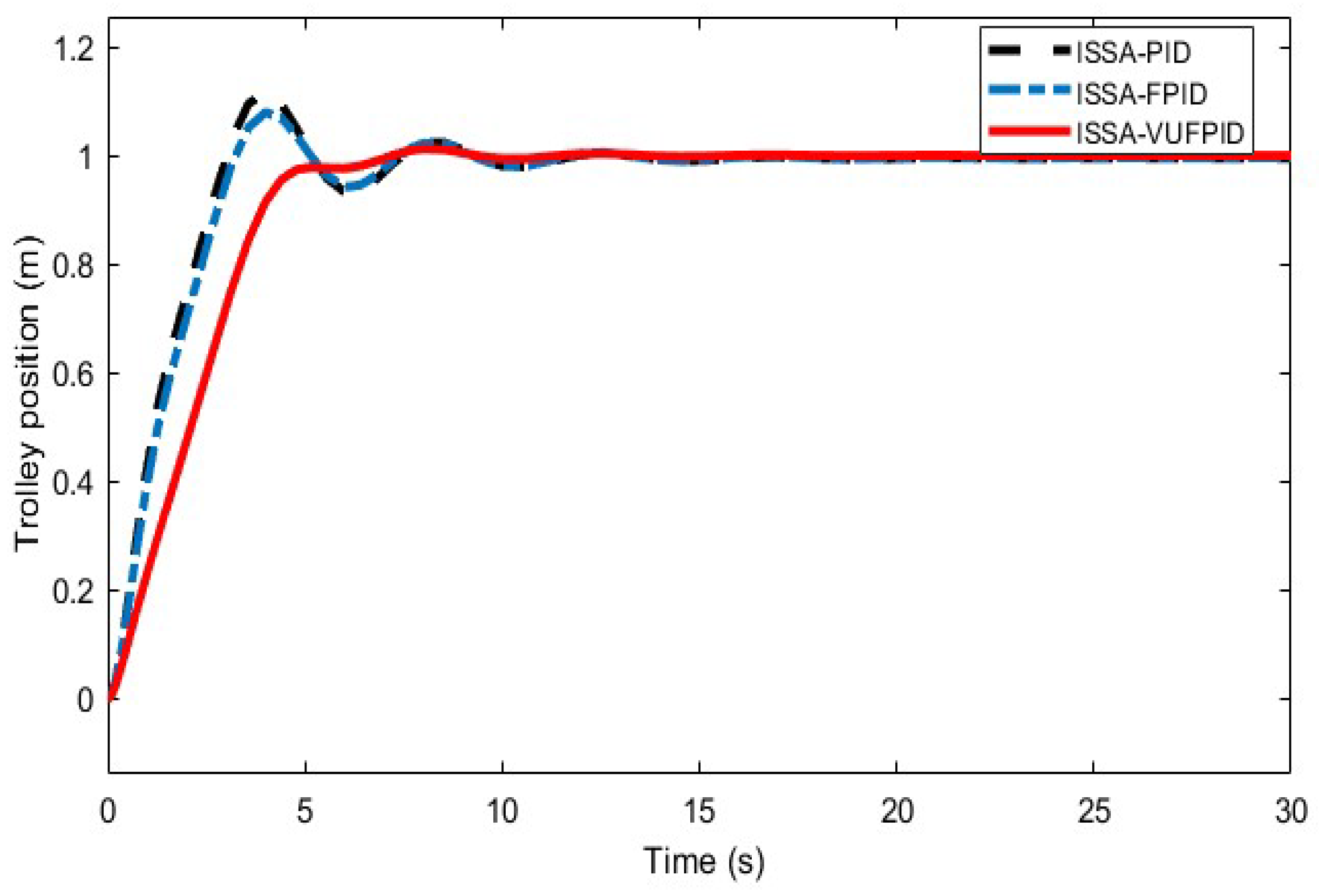
ISSA-PID	4.093	14.8%	14.172	0.991	0.0568	15.359
ISSA-FPID	4.046	10.7%	13.699	0.996	0.0532	13.356
ISSA-VUFPID	5.181	0%	5.371	0.997	0.0282	5.384

.

Figure 14 and Figure 15 demonstrate that after incorporating the ISSA and performing offline tuning, all three controllers show significant performance improvements. Compared with the PID and FPID controllers, the ISSA-PID and ISSA-FPID controllers improved overshoot suppression by 12.6% and 8.2%, respectively, and reduced settling times by 4.774 s and 3.355 s. In comparison to the VUFPID controller, the ISSA-VUFPID controller enhanced overshoot suppression by 6.9%, completely eliminating overshoot, and shortened the settling time by 7.901 s. Among the ISSA-tuned controllers, the ISSA-VUFPID controller exhibited the best overall performance. The experimental results show that the ISSA-VUFPID controller achieves superior control performance in the bridge crane system, especially in terms of precise trolley positioning and effective suppression of payload swing.

5.3. Robustness Simulation Experiments

In practical applications, variations in measurement techniques and environmental conditions can cause fluctuations in certain parameters of the bridge crane, potentially introducing errors. To assess the adaptability and stability of the three controllers, we conducted simulation tests of the crane control system under different operating conditions.

Table 12. Bridge crane control parameters for the other five working conditions.

Working Condition	Trolley Mass (kg)	Payload Mass (kg)	Cable Length (m)	Damping Coefficient (Ns/m)	Gravitational Acceleration (m/s2)
1	8	8	2	0.2	9.8
2	8	6	4	0.2	9.8
3	6	8	4	0.2	9.8
4	4	8	4	0.2	9.8
5	8	8	6	0.2	9.8

outlines these simulation scenarios along with their corresponding parameters.

Figure 16, Figure 17, Figure 18, Figure 19, Figure 20, Figure 21, Figure 22, Figure 23, Figure 24 and Figure 25 illustrate the curves of ISSA-PID, ISSA-FPID, and ISSA-VUFPID controllers in terms of trolley position control and payload swing under three operating conditions.

Table 13. Performance index of ISSA-PID, ISSA-FPID, and ISSA-VUFPID controllers under five working conditions.

Working Condition	Improved PID Controller	Trolley Position				Payload Swing Angle
		Peak Time (s)	Overshoot (%)	Steady-State Time (s)	Steady-State Value (m)	Max Angle (rad)	Steady State Time (s)
1	ISSA-PID	3.703	10.2%	9.905	0.9964	0.0629	10.763
	ISSA-FPID	3.892	6.1%	9.082	0.9961	0.0577	10.310
	ISSA-VUFPID	5.102	2.1%	7.333	1.0000	0.0281	9.902
2	ISSA-PID	3.987	15.1%	12.909	0.9953	0.0753	13.855
	ISSA-FPID	12.503	10.8%	12.351	0.9961	0.0688	13.107
	ISSA-VUFPID	8.861	0%	7.879	1.0000	0.0388	10.631
3	ISSA-PID	3.988	15.2%	13.821	0.9954	0.0598	15.485
	ISSA-FPID	4.038	11.1%	13.370	0.9960	0.0562	13.610
	ISSA-VUFPID	4.992	0%	5.393	1.0000	0.0287	7.920
4	ISSA-PID	3.975	13.6%	14.420	0.9952	0.0594	2.856
	ISSA-FPID	3.917	9.7%	13.839	0.9962	0.0598	2.817
	ISSA-VUFPID	5.193	0%	7.631	1.0000	0.0295	3.012
5	ISSA-PID	3.994	11.6%	16.144	0.9951	0.0882	19.113
	ISSA-FPID	4.031	7.9%	15.731	0.9965	0.0814	18.591
	ISSA-VUFPID	6.881	1.3%	9.281	1.0000	0.0405	12.748

summarizes the performance metrics for these controllers across the different scenarios. In the trolley position curves for conditions 1–5, the ISSA-VUFPID controller consistently achieves the desired setpoint with minimal payload swing, recording values of 0.0281, 0.0388, 0.0287, 0.0295, and 0.0405, respectively. In conditions 1 and 5, the ISSA-VUFPID controller exhibits a slight overshoot, which is 8% and 4% less than that of the ISSA-PID and ISSA-FPID controllers. In conditions 2, 3, and 4, the VUFPID controller shows zero overshoot and the fastest settling time. Regarding the payload swing curves across all three conditions, the ISSA-VUFPID controller demonstrates the smallest swing angle and shortest settling time, followed by the ISSA-FPID controller, with the ISSA-PID controller showing the largest values. In summary, while the ISSA-PID controller offers a fast response, it underperforms in suppressing overshoot and shortening recovery time, potentially leading to system instability. The ISSA-FPID controller shows improvements over ISSA-PID, particularly in reducing overshoot and settling time. However, the ISSA-VUFPID controller outperforms both ISSA-PID and ISSA-FPID in minimizing overshoot, achieving faster settling times, maintaining stable steady-state values, and reducing maximum swing angles. It is the most stable and precise control method among the three.

6. Conclusions

This paper presents a variable universe fuzzy PID controller enhanced by an advanced sparrow search algorithm (ISSA-VUFPID), designed to overcome the limitations associated with conventional fuzzy PID controllers, which often rely on expert knowledge for initial parameter settings and lack dynamic adaptation of the fuzzy universe. First, the quality of initial solutions is improved by incorporating tent map chaos into the initialization phase. Additionally, the algorithm incorporates a northern goshawk optimization phase to refine the positioning strategy, thereby increasing the thoroughness of the search within the solution space and accelerating the optimization process. Finally, an adaptive t-distribution perturbation strategy is used to adjust the position of sparrow followers, enhancing the algorithm’s optimization capability in the early search stages while focusing on local development in the later stages to improve solution accuracy. To validate the effectiveness of the proposed ISSA, it was compared with eight other optimization algorithms (SSA, NGO, DBO, GWO, GWCA, WOA, SABO, and RIME). The experimental results demonstrate that ISSA not only meets convergence requirements but also exhibits superior search precision, confirming its advantages. By introducing a nonlinear scaling factor in the FPID controller, the fuzzy domain range is dynamically adjusted. The performance of the VUFPID controller was compared with that of the PID and FPID controllers in the anti-sway and positioning control of the bridge crane, demonstrating the superiority of the VUFPID controller. ISSA was employed to initially parameter tune the PID controller. Compared with the ISSA-PID and ISSA-FPID controllers, the ISSA-VUFPID controller exhibited superior performance in controlling the trolley position and effectively suppressing payload swing angles. The ISSA-VUFPID controller demonstrated the best robustness and adaptability and is suitable for practical applications. The computational complexity of the ISSA-VUFPID could be higher compared with simpler PID or FPID controllers. Future work could focus on optimizing the algorithm to reduce computational overhead and testing its performance across a broader range of scenarios and applications to validate its effectiveness and robustness further.

References

- Yang, Y.; Jiang, H.; Gan, L.; Hua, C.; Li, J. Fixed-Time Composite Neural Learning Control of Flexible Telerobotic Systems. IEEE Trans. Cybern. 2024, 54, 3602–3614. [Google Scholar] [CrossRef] [PubMed]
- Deimel, R.; Brock, O. A novel type of compliant and underactuated robotic hand for dexterous grasping. Int. J. Robot. Res. 2015, 35, 161–185. [Google Scholar] [CrossRef]
- Liu, Y.; Lin, X.; Liu, Y.; Jiang, A.; Zhang, C. Affine formation maneuver control of underactuated surface vessels: Guaranteed safety under moving obstacles in narrow channels. Ocean. Eng. 2024, 303, 117721. [Google Scholar] [CrossRef]
- Mohammed, A.; Alghanim, K.; Andani, M.T. A robust input shaper for trajectory control of overhead cranes with non-zero initial states. Int. J. Dyn. Control 2021, 9, 230–239. [Google Scholar] [CrossRef]
- Adeli, M.; Zarabadipour, H.; Zarabadi, S.H.; Shoorehdeli, M.A. Anti-swing control for a double-pendulum-type overhead crane via parallel distributed fuzzy LQR controller combined with genetic fuzzy rule set selection. In Proceedings of the 2011 IEEE International Conference on Control System, Computing and Engineering, Penang, Malaysia, 25–27 November 2011; pp. 306–311. [Google Scholar]
- Jolevski, D.; Bego, O. Model predictive control of gantry/bridge crane with anti-sway algorithm. J. Mech. Sci. Technol. 2015, 29, 827–834. [Google Scholar] [CrossRef]
- Zhang, M.; Ma, X.; Rong, X.; Tian, X.; Li, Y. Adaptive tracking control for double-pendulum overhead cranes subject to tracking error limitation, parametric uncertainties and external disturbances. Mech. Syst. Signal Process. 2016, 76–77, 15–32. [Google Scholar] [CrossRef]
- Hou, C.; Liu, C.; Li, Z.; Xin, Z.; Zhang, H. Tower crane systems modeling and adaptive robust sliding mode control design under unknown frictions and wind disturbances. Trans. Inst. Meas. Control 2024, 01423312241260911. [Google Scholar] [CrossRef]
- Fujioka, D.; Singhose, W. Performance Comparison of Input-Shaped Model Reference Control on an Uncertain Flexible System. IFAC Pap. 2015, 48, 129–134. [Google Scholar] [CrossRef]
- Bozkurt, B.; Ertogan, M. Heave and horizontal displacement and anti-sway control of payload during ship-to-ship load transfer with an offshore crane on very rough sea conditions. Ocean. Eng. 2023, 267, 113309. [Google Scholar] [CrossRef]
- Yan, Y.; Qin, Y.-X.; Zhang, L.-S.; Jia, T.; Sun, F. Swing Suppression Control in Quayside Crane by Using Fuzzy Logic and Improved Particle Swarm Optimization Algorithm. Iran. J. Sci. Technol. Trans. Mech. Eng. 2023, 47, 1131–1144. [Google Scholar] [CrossRef]
- Liu, L.; Zhang, Y.; Chen, J.; Chen, J. Research and Application of Control Algorithm Based on Intelligent Traveling Crane. In Proceedings of the 2023 IEEE 13th International Conference on CYBER Technology in Automation, Control, and Intelligent Systems (CYBER), Qinhuangdao, China, 11–14 July 2023; pp. 148–153. [Google Scholar]
- Yu, Z.; Dong, H.-M.; Liu, C.-M. Research on Swing Model and Fuzzy Anti Swing Control Technology of Bridge Crane. Machines 2023, 11, 579. [Google Scholar] [CrossRef]
- El-Nagar, A.M.; El-Bardini, M. Parallel realization for self-tuning interval type-2 fuzzy controller. Eng. Appl. Artif. Intell. 2017, 61, 8–20. [Google Scholar] [CrossRef]
- Fu, J.; Liu, J.; Xie, D.; Sun, Z. Application of Fuzzy PID Based on Stray Lion Swarm Optimization Algorithm in Overhead Crane System Control. Mathematics 2023, 11, 2170. [Google Scholar] [CrossRef]
- Sałabun, W.; Więckowski, J.; Shekhovtsov, A.; Palczewski, K.; Jaszczak, S.; Wątróbski, J. How to Apply Fuzzy MISO PID in the Industry? An Empirical Study Case on Simulation of Crane Relocating Containers. Electronics 2020, 9, 2017. [Google Scholar] [CrossRef]
- Zeng, W.; Jiang, Q.; Xie, J.; Yu, T. A functional variable universe fuzzy PID controller for load following operation of PWR with the multiple model. Ann. Nucl. Energy 2020, 140, 107174. [Google Scholar] [CrossRef]
- Yang, S.; Deng, B.; Wang, J.; Liu, C.; Li, H.; Lin, Q.; Fietkiewicz, C.; Loparo, K.A. Design of Hidden-Property-Based Variable Universe Fuzzy Control for Movement Disorders and Its Efficient Reconfigurable Implementation. IEEE Trans. Fuzzy Syst. 2019, 27, 304–318. [Google Scholar] [CrossRef]
- Mingxue, L.; Guolai, Y.; Xiaoqing, L.; Guixiang, B. Variable Universe Fuzzy Control of Adjustable Hydraulic Torque Converter Based on Multi-Population Genetic Algorithm. IEEE Access 2019, 7, 29236–29244. [Google Scholar] [CrossRef]
- Liu, G.; Jiang, W.; Wang, Q.; Wang, T. Enhanced variable universe fuzzy proportional–integral–derivative control of structural vibration with real-time adaptive contracting–expanding factors. J. Vib. Control. 2021, 28, 1962–1975. [Google Scholar] [CrossRef]
- Xue, J.; Shen, B. A novel swarm intelligence optimization approach: Sparrow search algorithm. Syst. Sci. Control. Eng. 2020, 8, 22–34. [Google Scholar] [CrossRef]
- Liu, J.; Wang, Z. Artificial immune algorithm-sparrow search algorithm and its application in network intrusion detection. J. Intell. Fuzzy Syst. 2022, 43, 5001–5011. [Google Scholar] [CrossRef]
- Liu, L.; Liang, J.; Guo, K.; Ke, C.; He, D.; Chen, J. Dynamic Path Planning of Mobile Robot Based on Improved Sparrow Search Algorithm. Biomimetics 2023, 8, 182. [Google Scholar] [CrossRef] [PubMed]
- Gao, B.; Shen, W.; Guan, H.; Zheng, L.; Zhang, W. Research on Multistrategy Improved Evolutionary Sparrow Search Algorithm and its Application. IEEE Access 2022, 10, 62520–62534. [Google Scholar] [CrossRef]
- Xiong, Q.; Zhang, X.; He, S.; Shen, J. A Fractional-Order Chaotic Sparrow Search Algorithm for Enhancement of Long Distance Iris Image. Mathematics 2021, 9, 2790. [Google Scholar] [CrossRef]
- Chen, Y.-J.; Huang, H. A novel conceptual design approach for autonomous underwater helicopter based on multidisciplinary collaborative optimization. Eng. Appl. Comput. Fluid Mech. 2024, 18, 2325494. [Google Scholar] [CrossRef]
- Dehghani, M.Š.H.; Trojovský, P. Northern Goshawk Optimization: A New Swarm-Based Algorithm for Solving Optimization Problems. IEEE Access 2021, 9, 162059–162080. [Google Scholar] [CrossRef]
- Huang, X.; Wang, S.; Lu, T.; Li, H.; Wu, K.; Deng, W. Chloride Permeability Coefficient Prediction of Rubber Concrete Based on the Improved Machine Learning Technical: Modelling and Performance Evaluation. Polymers 2023, 15, 308. [Google Scholar] [CrossRef]
- Ouyang, M.; Wang, Y.; Wu, F.; Lin, Y. Continuous Reactor Temperature Control with Optimized PID Parameters Based on Improved Sparrow Algorithm. Processes 2023, 11, 1302. [Google Scholar] [CrossRef]
- Xue, J.; Shen, B. Dung beetle optimizer: A new meta-heuristic algorithm for global optimization. J. Supercomput. 2023, 79, 7305–7336. [Google Scholar] [CrossRef]
- Mirjalili, S.; Mirjalili, S.M.; Lewis, A. Grey Wolf Optimizer. Adv. Eng. Softw. 2014, 69, 46–61. [Google Scholar] [CrossRef]
- Guan, Z.; Ren, C.; Niu, J.; Wang, P.; Shang, Y. Great Wall Construction Algorithm: A novel meta-heuristic algorithm for engineer problems. Expert Syst. Appl. 2023, 233, 120905. [Google Scholar] [CrossRef]
- Mirjalili, S.; Lewis, A. The Whale Optimization Algorithm. Adv. Eng. Softw. 2016, 95, 51–67. [Google Scholar] [CrossRef]
- Trojovský, P.; Dehghani, M. Subtraction-Average-Based Optimizer: A New Swarm-Inspired Metaheuristic Algorithm for Solving Optimization Problems. Biomimetics 2023, 8, 149. [Google Scholar] [CrossRef] [PubMed]
- Su, H.; Zhao, D.; Heidari, A.A.; Liu, L.; Zhang, X.; Mafarja, M.; Chen, H. RIME: A physics-based optimization. Neurocomputing 2023, 532, 183–214. [Google Scholar] [CrossRef]
- Li, H.; Hui, Y.; Ma, J.; Wang, Q.; Zhou, Y.; Wang, H. Research on Variable Universe Fuzzy Multi-Parameter Self-Tuning PID Control of Bridge Crane. Appl. Sci. 2023, 13, 4830. [Google Scholar] [CrossRef]