Interval Constrained Multi-Objective Optimization Scheduling Method for Island-Integrated Energy Systems Based on Meta-Learning and Enhanced Proximal Policy Optimization

Abstract

Multiple uncertainties from source–load and energy conversion significantly impact the real-time dispatch of an island integrated energy system (IIES). This paper addresses the day-ahead scheduling problems of IIES under these conditions, aiming to minimize daily economic costs and maximize the output of renewable energies. We introduce an innovative algorithm for Interval Constrained Multi-objective Optimization Problems (ICMOPs), which incorporates meta-learning and an improved Proximal Policy Optimization with Clipped Objective (PPO-CLIP) approach. This algorithm fills a notable gap in the application of DRL to complex ICMOPs within the field. Initially, the multi-objective problem is decomposed into several single-objective problems using a uniform weight decomposition method. A meta-model trained via meta-learning enables fine-tuning to adapt solutions for subsidiary problems once the initial training is complete. Additionally, we enhance the PPO-CLIP framework with a novel strategy that integrates probability shifts and Generalized Advantage Estimation (GAE). In the final stage of scheduling plan selection, a technique for identifying interval turning points is employed to choose the optimal plan from the Pareto solution set. The results demonstrate that the method not only secures excellent scheduling solutions in complex environments through its robust generalization capabilities but also shows significant improvements over interval-constrained multi-objective evolutionary algorithms, such as IP-MOEA, ICMOABC, and IMOMA-II, across multiple multi-objective evaluation metrics including hypervolume (HV), runtime, and uncertainty.

1. Introduction

As environmental concerns escalate and energy resources dwindle, countries around the world are proactively pushing for energy reform to lessen their reliance on traditional energy sources like fossil fuels [1,2]. An IIES enhances this effort by blending diverse renewable and conventional energy sources [3,4,5,6]. These systems employ advanced technologies for energy conversion, storage, and smart management to create an efficient, reliable, and sustainable supply chain. An IIES manages the scheduling of wind, solar, and wave energy to fulfill the needs for electricity, cooling, heating, and water supply. The primary challenges faced by IIESs in daily scheduling plans include the uncertainty and variability of renewable energy sources, inaccuracies in load forecasting, limited energy storage capacity, and complex energy management and scheduling strategies.

To manage these uncertainties, several optimization strategies have been explored, including robust [7], stochastic [8,9], and interval optimization [10,11]. Robust optimization ensures stability by planning for worst-case scenarios, leading to potentially conservative and inefficient resource utilization. Stochastic optimization, which relies on accurate probability distributions and extensive scenario analysis, increases model accuracy but demands significant computational resources and accurate historical data. Interval optimization offers a middle ground by directly setting ranges for uncertainties, thus simplifying the model at lower computational costs, though its accuracy highly depends on how these ranges are set. Given the multiple uncertainties IIESs face, such as extreme weather, unstable energy supply, and variable demands, interval optimization emerges as a flexible approach to tackle these challenges. This paper, therefore, explores the application of interval optimization to the multi-objective scheduling problems of IIES, identified as ICMOP.

The approaches currently available for tackling interval-constrained multi-objective optimization problems remain limited [12,13,14,15,16,17,18]. Chen [17] et al. introduced a novel NSGA-II algorithm for ICMOPs, which employs interval possibility and interval crowding distance to define interval dominance relationships. Meanwhile, Zeng [18,19,20] et al. developed an individual selection strategy with interval constraints to tackle the optimization configuration and scheduling of a renewable energy system with five substations. Yu [21] et al. developed a penalty function-based interval-constrained multi-objective optimization algorithm, which effectively addresses interval constraints in uncertain scenarios using interval analysis and innovative penalty functions. However, the computational complexity of ICMOEA is considerable, especially in large-scale implementations, requiring extensive computational resources and time.

In the study of IIES, most research only considers the uncertainties of renewable energy output and load demand. However, if the uncertainties in the conversion efficiency of various energy-side devices are also taken into account, this would significantly increase the difficulty of real-time scheduling [22]. Previous research methodologies have primarily focused on cost minimization, often overlooking these uncertainties, thereby limiting the practical application of the models. Furthermore, although ICMOPs have been extensively discussed theoretically, existing multi-objective evolutionary algorithms demonstrate considerable deficiencies in processing speed and generalization capability. Specifically, methods based on DRL, though widely applied in single-objective optimization, are still in their nascent stages in multi-objective optimization research, with interval multi-objective optimization representing a particularly challenging branch that has yet to be explored in the context of IIES [23].

In light of these challenges, this study introduces an MOMAML-PPO algorithm, which integrates meta-learning with an enhanced version of PPO-CLIP [24], aiming to bridge this research gap. The primary objective of this paper is to address the real-time scheduling issues of IIES, with specific innovations including the following: (1) IIES model architecture: Utilizing prediction errors and confidence interval estimation, this study models the uncertainties of sources, energy conversions, and loads with interval descriptions. The model aims to minimize economic costs and maximize renewable energy output for an island’s integrated energy system. (2) Introduction of meta-learning: By employing meta-learning techniques to train a meta-model, it can, after solving one sub-model, adapt to other models’ solutions through mere fine-tuning [25]. The incorporation of meta-learning not only enhances the model’s generalizability but also significantly reduces the transition time between different models, thereby improving overall solution efficiency. (3) Enhancements to PPO-CLIP: By integrating probability shifts and Generalized Advantage Estimation (GAE), the stability and exploratory capabilities of policy updates are strengthened, particularly in the data-constrained environments of IIES. (4) Precision selection technique for solutions: Utilizing interval breakpoint identification techniques, this strategy sifts through the Pareto solution set to select the optimal scheduling plans, thereby further enhancing the economic efficiency and reliability of the final scheduling solutions.

2. An Optimal Scheduling Model for IIES Based on Multiple Uncertainties

2.1. Previous Research

In the challenging landscape of integrated energy system (IES) optimization and scheduling, multifaceted uncertainties, such as fluctuations in sources and loads, profoundly impact system stability. Extant research has centered on these uncertainties, exploring resolution through diverse mathematical models and optimization strategies. For instance, Hu [26] employed interval planning theory and stochastic analysis to construct a planning model for an energy system with multiple uncertainties, leveraging fuzzy sets and feasibility analysis. This model, aiming at economic minimization, achieved optimal system scheduling, although its applicability remains limited to specific scenarios. Meanwhile, Bai [27] developed a two-layer robust optimization scheduling model based on extreme scenarios of wind power output. This model uses a column constraint generation algorithm for iterative solutions, effectively addressing the regulation costs induced by wind power uncertainties.

On another note, Zhang [28] targeted the uncertainties of cold, heat, and electricity loads using Monte Carlo simulations to generate uncertain parameter scenarios, subsequently reducing the number of scenarios through reverse scenario reduction techniques for long-term planning. Despite these efforts, scenario generation techniques have not fully integrated system scheduling with load uncertainties. Furthermore, Zheng [29] introduced an interval multi-objective scheduling model that transforms into a deterministic optimization problem via interval ordering relations and possibility methods, solved using an improved non-dominated sorting genetic algorithm. These studies collectively reveal that current IES optimization scheduling heavily relies on the modeling or predictive accuracy of renewable sources and load uncertainties, inadequately addressing equipment conversion efficiency and the complexities of real-world scenarios.

With the increasing scale of problems, traditional evolutionary learning methods struggle to ensure the rapid response required for real-time scheduling. In this context, DRL has emerged as a novel solution. For example, Wang [30] applied scenario analysis to model the stochasticity of wind turbines and photovoltaics, utilizing Generative Adversarial Networks to learn the intermittent characteristics of renewable energy outputs, thus producing more realistic typical scenarios. Yan [31] implemented the soft actor–critic (SAC) algorithm, focusing on real-time electricity pricing and the remaining battery capacity of electric vehicles to develop intelligent charging strategies. Wu [32] introduced a phased training approach using a Double Deep Q-Network (D3QN) [33] in the real-time scheduling model of IES, effectively mitigating the issue of oversized action spaces in traditional RL methods.

Currently, DRL is primarily applied to straightforward scheduling issues in island-based integrated energy systems, with scarce research extending it to the relatively complex problems of ICMOPs [34,35]. To address this gap, this study proposes modeling the operational scheduling problem of island-integrated energy systems as ICMOPs, solved using the MOMAML-PPO method. This approach is anticipated to comprehensively handle multiple uncertainties while ensuring the minimization of costs and the maximization of renewable energy outputs.

2.2. IIES Architecture

This paper utilizes a structure for the IIES, as illustrated in Figure 1 [36,37,38]. The architecture primarily encompasses the following components: renewable energy generation using wind, photovoltaic, and wave energy; an energy conversion section, including electrolytic cells (ECs), hydrogen tanks (HTs), hydrogen fuel cells (HFCs), electric boilers (EBs), electric refrigerators (ERs), adsorption refrigerators (ARs), water source heat pumps (WSHPs), and seawater desalination systems (SDs); and the user side, which covers four types of energy loads: electrical, cooling, heating, and water.

In this system, wind, photovoltaic, and wave energies are captured and converted into electrical energy. Some of the electrical energy is transformed into hydrogen through the EC and stored and then reconverted into electricity by the HFC. The EB and WSHP are used to meet heating demands, the ER and AR fulfill cooling needs, and the SD system addresses water load requirements.

In this study, we addressed the uncertainties stemming from renewable energy output, diverse load demands, and the energy conversion efficiencies of various coupled devices. To predict the output of renewable energy and load forecasts, we employ a method of error feedback and confidence intervals [36,37]. The output and load forecasts are described as interval numbers, using historical data’s sample mean and variance to calculate a 95% confidence interval of the overall mean [38,39]. This estimation helps better account for the potential fluctuations in actual renewable energy output and loads, considering the uncertainties more effectively. In terms of energy conversion, which involves equipment like EC, HT, HFC, EB, ER, AR, WSHP, and SD Units, we consider uncertainties such as energy conversion efficiency to build corresponding uncertainty models, ensuring stability and reliability in the energy conversion process.

2.2.1. Electrical Load

In the study of power output predictions from wind, solar, and wave energy generation, the outputs are influenced by variables, such as wind speed, temperature, and other environmental factors, all of which introduce uncertainties. To represent these uncertainties, we use interval numbers to express the predicted output of each renewable energy source during specific intervals. These intervals include predictions based on historical data and adjustments for forecast errors and environmental noise. Specifically, the output interval for wind energy can be represented as follows:

$${\left[P_{wind}\left(t\right)\right]}^{\pm }=\left[\begin{array}{c}{P}_{wind}\left(t\right)-\left(MS{E}_{wind}\left(t\right)+{\epsilon }_{wind}\left(t\right)\right),\\ P_{wind}\left(t\right)+\left(MS{E}_{wind}\left(t\right)+{\epsilon }_{wind}\left(t\right)\right)\end{array}\right].$$

(1)

where ${\left[P_{wind}\left(t\right)\right]}^{\pm }$ represents the wind power output interval at time $t$. $P_{wind}\left(t\right)$ denotes the wind power output predicted based on historical data, $MS{E}_{wind}\left(t\right)$ is the mean squared error at time $t$, and ${\epsilon }_{wind}\left(t\right)$ represents the random perturbation due to environmental factors at time $t$. The output intervals for solar and wave energy are defined similarly and, therefore, not repeated here.

The electrolysis of water into hydrogen using electricity not only stores energy but also addresses the intermittency and uncertainties of renewable sources. However, the efficiency of the water electrolysis process is influenced by various factors, such as ambient temperature and system external conditions, which induce uncertainties in the hydrogen production rate. To quantify this process, we have established the following mathematical model:

$${\left[V_{H_2}\left(t\right)\right]}^{\pm }={\displaystyle \frac{{\tau }_{H_2}{P}_{H_2}\left(t\right){\rho }_{H_2}}{4M_{H_2}{\left[{\nu }_{H_2}\right]}^{\pm }}}.$$

(2)

where ${\left[V_{H_2}\left(t\right)\right]}^{\pm }$ represents the interval value of the hydrogen volume produced by the EC at time $t$, $P_{H_2}\left(t\right)$ is the electrical power consumed by the EC during that period, ${\tau }_{H_2}$ is the conversion coefficient of the EC, ${\rho }_{H_2}$ is the density of hydrogen, ${\left[{\nu }_{H_2}\right]}^{\pm }$ is the interval value for the rate of hydrogen production by water electrolysis, and $M_{H_2}$ is the molar mass of hydrogen.

The storage of hydrogen is also subject to uncertainties, and its dynamic changes can be represented by the following model:

$${\left[S_{H_2}\left(t\right)\right]}^{\pm }={\left[S_{H_2,in}\left(t\right)\right]}^{\pm }-{\left[S_{H_2,out}\left(t\right)\right]}^{\pm }+{\left[S_{H_2}\left(t-1\right)\right]}^{\pm }.$$

(3)

where ${\left[S_{H_2}\left(t\right)\right]}^{\pm }$ represents the interval value of the hydrogen storage amount at time $t$, ${\left[S_{H_2,in}\left(t\right)\right]}^{\pm }$ and ${\left[S_{H_2,out}\left(t\right)\right]}^{\pm }$ represent the intervals of hydrogen input and output during that period, respectively, $\left[S_{H_2}\left(t-1\right)\right]$ represents the interval value of hydrogen storage from the previous period, with $t-1$ serving as the starting baseline for the current period.

For HFC, which operate as the reverse process of water electrolysis using hydrogen as fuel to generate electricity, the efficiency of HFC also possesses uncertainties. The corresponding mathematical model is expressed as follows:

$${\left[P_{hf}\left(t\right)\right]}^{\pm }={\left[{\eta }_{hf}\right]}^{\pm }{V}_{hf}\left(t\right)H_{hv}.$$

(4)

where ${\left[P_{hf}\left(t\right)\right]}^{\pm }$ represents the interval value of electrical power generated by the hydrogen fuel cell at time $t$, ${\left[{\eta }_{hf}\right]}^{\pm }$ is the efficiency interval of the hydrogen fuel cell, $V_{hf}\left(t\right)$ is the volume of hydrogen consumed by the fuel cell during that period, and $H_{hv}$ is the higher heating value of hydrogen.

2.2.2. Cooling Load

In the performance study of absorption refrigerators, the primary issue we encounter is the uncertainty of the cooling coefficient. To quantify this uncertainty, the following mathematical model is established:

At any given time $t$, the cooling power $C_{AC}\left(t\right)$ of the absorption refrigerator can be expressed as the product of the consumed thermal power $H_{AC}\left(t\right)$ and the cooling coefficient $CO{P}_{ac}$, where the cooling coefficient has a certain range of uncertainty. The model is specifically represented as follows:

$${\left[C_{ac}\left(t\right)\right]}^{\pm }=H_{ac}\left(t\right){\left[CO{P}_{ac}\right]}^{\pm }.$$

(5)

Further, changes in the cooling power affect the freshwater usage $W_{AC}\left(t\right)$ of the refrigerator, which also exhibits uncertainty and can be estimated through the product of the water consumption rate ${\eta }_{AC}$ and the cooling power:

$${\left[W_{ac}\left(t\right)\right]}^{\pm }={\left[C_{ac}\left(t\right)\right]}^{\pm }{\left[{\eta }_{ac}\right]}^{\pm }.$$

(6)

where ${\left[C_{AC}\left(t\right)\right]}^{\pm }$, $H_{AC}\left(t\right)$, and ${\left[W_{AC}\left(t\right)\right]}^{\pm }$ represent the interval values of the cooling power, the consumed thermal power, and the freshwater usage of the absorption refrigerator at time $t$, respectively. ${\left[C_{AC}\left(t\right)\right]}^{\pm }$ and ${\left[{\eta }_{AC}\right]}^{\pm }$ indicate the interval values of the cooling coefficient and the water consumption rate, respectively.

2.2.3. Heating Load

In analyzing the thermal energy conversion processes of WSHP and EB, it is crucial to account for the uncertainties introduced by environmental factors to precisely assess the performance fluctuations of these devices under varying operating conditions. The model incorporates the conversion of high-quality electrical energy into high-quality thermal energy during any given period $t$. The model is represented as follows:

$${\left[P_{wshp,h}\left(t\right)\right]}^{\pm }=P_{wshp}\left(t\right){\left[{\eta }_{wshp,h}\right]}^{\pm },$$

(7)

$${\left[W_{wshp}\left(t\right)\right]}^{\pm }=P_{wshp}\left(t\right){\left[{\eta }_{wshp}\right]}^{\pm }.$$

(8)

where ${\left[P_{wshp,h}\left(t\right)\right]}^{\pm }$ and ${\left[W_{wshp}\left(t\right)\right]}^{\pm }$ represent the interval values of the heating power and the freshwater usage of the water source heat pump at time $t$. $P_{wshp}\left(t\right)$ indicates the heating power of the water source heat pump during period $t$, including consumed high-quality electrical energy and the interval values of freshwater usage. ${\left[{\eta }_{wshp,h}\right]}^{\pm }$ and ${\left[{\eta }_{wshp}\right]}^{\pm }$ are the interval values of the heating efficiency coefficient and the water consumption rate, respectively. Considering the uncertainty in the heating efficiency of EB, the uncertainty mathematical model is established as follows:

$${\left[P_{eb,h}\left(t\right)\right]}^{\pm }=P_{eb}\left(t\right){\left[{\eta }_{eb}\right]}^{\pm }.$$

(9)

where ${\left[P_{eb,h}\left(t\right)\right]}^{\pm }$ represents the heating power interval value of the electric boiler during period $t$, and ${\left[{\eta }_{eb}\right]}^{\pm }$ indicates the interval value of the heating efficiency of the EB.

2.2.4. Water Load

In response to the scarcity of freshwater resources in island regions, seawater desalination units provide an effective solution. These units convert seawater into potable freshwater through the desalination process, which is critical for the survival and development of island communities. However, the water production rate during the desalination process is uncertain, necessitating precise mathematical modeling for its description and management. Below is the mathematical model for a seawater desalination unit considering the uncertainty of the water production rate:

$${\left[W_{du,w}\left(t\right)\right]}^{\pm }=P_{du}\left(t\right){\left[{\eta }_{du}\right]}^{\pm }.$$

(10)

where ${\left[W_{du,w}\left(t\right)\right]}^{\pm }$ represents the interval values of the freshwater volume produced by the seawater desalination unit during period $t$, $P_{du}\left(t\right)$ denotes the electrical power consumed by the desalination unit in the same period, and ${\left[{\eta }_{du}\right]}^{\pm }$ indicates the interval values of the water production rate of the desalination unit.

2.3. Objective Function

For the proposed integrated energy system model of the island, this study addresses the optimization scheduling problem of the types and numbers of renewable energy output devices over a 24 h cycle with a time step of 1 h. The objective functions aim to minimize the economic cost within the cycle and maximize the renewable energy output.

2.3.1. Economic Cost Minimization

The total system cost interval value for a scheduling period ${\left[F_1\right]}^{\pm }$ is composed of the maintenance cost interval value ${\left[F_{mc}\right]}^{\pm }$ and the variable cost interval value ${\left[F_{cc}\right]}^{\pm }$:

$${\min \left[F_1\right]}^{\pm }={\left[F_{mc}\right]}^{\pm }+{\left[F_{cc}\right]}^{\pm }.$$

(11)

The maintenance cost interval for time $t$, denoted as ${\left[F_{mc}\right]}^{\pm }$, is represented as follows:

$${\left[F_{mc}\right]}^{\pm }={\displaystyle \sum _{t=1}^T}\sum _i\sum _j\left(x_{i,j}\left(t\right)C_{i,j}\right)+{\displaystyle \sum _{t=1}^T}{\left[P_{eov}\right]}^{\pm }{C}_{eov}.$$

(12)

where $x_{i,j}\left(t\right)$ represents the number of operational units of the $j^{th}$ specification of the $i^{th}$ type of energy resource at time $t$, and $C_{i,j}$ represents the maintenance cost of the $j^{th}$ specification of the $i^{th}$ type of energy resource. ${\sum }_{t=1}^T{\left[P_{eov}\right]}^{\pm }$ represents the interval value of the unit output during period $t$, and $C_{eov}$ denotes the unit maintenance cost per period $t$.

The variable cost interval for time $t$, denoted as ${\left[F_{cc}\left(t\right)\right]}^{\pm }$, is represented as follows:

$${\left[F_{cc}\left(t\right)\right]}^{\pm }={\left[P_{cwp}\left(t\right)\right]}^{\pm }{C}_{pucpc}.$$

(13)

where ${\left[P_{cwp}\left(t\right)\right]}^{\pm }$ represents the interval value of the variable power for period $t$, and $C_{pucpc}$ indicates the unit cost of variable charges.

2.3.2. Maximization of Renewable Energy Output

The interval value of renewable energy output for a scheduling period ${\left[F_2\right]}^{\pm }$:

$${\max \left[F_2\right]}^{\pm }={\displaystyle \sum _{t=1}^T}\sum _i\sum _j\left({N_{i,j}\left[P_{i,j}\left(t\right)\right]}^{\pm }\right).$$

(14)

where $N_{i,j}$ represents the number of units of each specification of renewable energy sources during period $t$, and $\left[P_{i,j}{\left(t\right)}^{\pm }\right]$ indicates the interval value of the output for each renewable energy device during period $t$.

2.4. Constraint Function

The constraints of the uncertainty-based multi-objective optimization scheduling model for the island’s integrated energy system ensure that the system operates safely, reliably, and economically while finding an optimal balance between multiple objectives (minimizing economic costs and maximizing renewable energy output).

2.4.1. Integrated Energy System Power Constraints

Power balance in the integrated energy system is crucial for stable operation. The output of various energy sources must meet the following balance constraints:

$$\left\{\begin{array}{l}{\left[Q_{electric}\right]}^{\pm }=\left({\left[P_{water}\left(t\right)\right]}^{\pm }+{\left[P_{solar}\left(t\right)\right]}^{\pm }+{\left[P_{wave}\left(t\right)\right]}^{\pm }\right)\\ \hspace{1em}\left({\left[P_{eb}\left(t\right)\right]}^{\pm }+{\left[P_{ec}\left(t\right)\right]}^{\pm }+{\left[P_{du}\left(t\right)\right]}^{\pm }+{\left[P_{wshp}\left(t\right)\right]}^{\pm }\right)\\ {\left[Q_{cooling}\right]}^{\pm }={\left[C_{ec}\left(t\right)\right]}^{\pm }+{\left[C_{ac}\left(t\right)\right]}^{\pm }\\ {\left[Q_{heating}\right]}^{\pm }={\left[P_{wshp,h}\left(t\right)\right]}^{\pm }+{\left[P_{eb,h}\left(t\right)\right]}^{\pm }-{\left[H_{ac,h}\left(t\right)\right]}^{\pm }\\ {\left[Q_{water}\right]}^{\pm }={\left[W_{du,w}\left(t\right)\right]}^{\pm }-{\left[W_{wshp}\left(t\right)\right]}^{\pm }-{\left[W_{ac}\left(t\right)\right]}^{\pm }\end{array}.\right.$$

(15)

where ${\left[Q_{electric}\right]}^{\pm }$, ${\left[Q_{heating}\right]}^{\pm }$, ${\left[Q_{heating}\right]}^{\pm }$, and ${\left[Q_{water}\right]}^{\pm }$ represent the electric, cooling, heating, and water loads for period $t$, respectively.

2.4.2. Renewable Energy Output Constraints

The output of renewable energies is constrained by upper and lower limits to ensure the stability and reliable operation of the system. Specifically, the outputs for wind, solar, and wave energy at any time tt are subjected to the following constraints:

$$0\le {\left[P_{wind}\left(t\right)\right]}^{\pm }\le P_{wind,max}\left(t\right),$$

(16)

$$0\le {\left[P_{solar}\left(t\right)\right]}^{\pm }\le P_{solar,max}\left(t\right),$$

(17)

$$0\le {\left[P_{wave}\left(t\right)\right]}^{\pm }\le P_{wave,max}\left(t\right).$$

(18)

where $P_{wind,max}\left(t\right)$, $P_{solar,max}\left(t\right)$, and $P_{wave,max}\left(t\right)$, respectively, represent the maximum permissible outputs for wind, solar, and wave energy sources for period $t$. These constraints help maintain balance and prevent overloading of the system, ensuring optimal and sustainable operation.

2.4.3. Renewable Energy Units Count Constraint

To appropriately allocate resources and optimize system performance, the number of renewable energy units within the island’s integrated energy system is subject to specific limits. The number of units for wind, solar, and wave energy output devices are $N_{wind}$, $N_{solar}$, and $N_{wave}$, respectively, and must satisfy the following conditions:

$$0\le N_{wind}\le N_{wind,max},$$

(19)

$$0\le N_{solar}\le N_{solar,max},$$

(20)

$$0\le N_{wave}\le N_{wave,max}.$$

(21)

where $N_{wind,max}$, $N_{solar,max}$, and $N_{wind,max}$ represent the maximum allowable number of units for wind, solar, and wave energy, respectively. These constraints are set to ensure that the deployment of renewable energy sources is within the sustainable capacity of the island’s environment and infrastructure.

2.4.4. Unit Ramp Rate Constraint

To ensure smooth transitions in power changes within the system, the output of coupled devices must remain within a specified range, and their ramp rates are also limited. The specific constraints are as follows:

$$P_i^{min}\le {\left[P_i\left(t\right)\right]}^{\pm }\le P_i^{max\left(t\right)},$$

(22)

$${-{\varsigma }_i^{min}\le \left[P_i\left(t\right)\right]}^{\pm }-\left[P_i\left(t-1\right)\right]\le {\varsigma }_i^{max}.$$

(23)

where $P_i^{min\left(t\right)}$ and $P_i^{max\left(t\right)}$ denote the lower and upper output limits for device $i$, and ${\varsigma }_i^{min}$ and ${\varsigma }_i^{max}$ represent the downward and upward ramp rates, respectively. These ramp rate constraints help to mitigate any abrupt changes in power output, which can be critical for maintaining grid stability and ensuring the reliability of power supply on the island.

2.4.5. Operational Constraints of HFC Energy Storage Systems

During the operation of hydrogen fuel cell energy storage systems, specific constraints on storage capacity and charging/discharging power must be satisfied to ensure efficient and safe functioning. These operational constraints are defined as follows:

$$\left\{\begin{array}{l}{P}_{q,in}^{\min }\left(t\right)\le {\left[P_{q,in}\left(t\right)\right]}^{\pm }\le P_{q,in}^{\max }\left(t\right)\\ P_{q,out}^{\min }\left(t\right)\le {\left[P_{q,out}\left(t\right)\right]}^{\pm }\le P_{q,out}^{\max }\left(t\right)\\ E_q^{min}\left(t\right)\le {\left[E_q\left(t\right)\right]}^{\pm }\le E_q^{max}\left(t\right)\\ {\left[E_q\left(t\right)\right]}^{\pm }={\left[SE{E}_{q,static}\left(t\right)\right]}^{\pm }\\ {\left[E_q\left(t\right)\right]}^{\pm }={\left[SE{E}_{q,in}\left(t\right)\right]}^{\pm }{\left[P_{q,in}\left(t\right)\right]}^{\pm }{\left[CD{E}_{q,in}\right]}^{\pm }-{\displaystyle \frac{{\left[SE{E}_{q,out}\left(t\right)\right]}^{\pm }{\left[P_{q,out}\left(t\right)\right]}^{\pm }}{{\left[CD{E}_{q,out}\right]}^{\pm }}}\end{array}\right..$$

(24)

where $E_q^{min\left(t\right)}$ and $E_q^{max\left(t\right)}$ represent the lower and upper limits of the storage capacity for the time period $t$, respectively. $P_{q,in}^{\min }\left(t\right)$, $P_{q,in}^{\max }\left(t\right)$, $P_{q,out}^{\min }\left(t\right)$, and $P_{q,out}^{\max }\left(t\right)$ represent the lower and upper limits of the power for charging and discharging for the time period $t$. ${\left[SE{E}_{q,static}\left(t\right)\right]}^{\pm }$ denotes the static energy efficiency interval of the storage device during the time period $t$, and ${\left[CD{E}_{q,in}\right]}^{\pm }$ and ${\left[CD{E}_{q,out}\right]}^{\pm }$ represent the charging and discharging efficiency intervals, respectively.

3. Interval-Constrained Multi-Objective Optimization Algorithm Based on DRL

3.1. MOMAML-PPO Solution Process

This study employs the MOMAML-PPO algorithm to address the multi-objective interval-constrained optimization scheduling issues in integrated island energy systems. As illustrated in Figure 2, this research initially constructs a model of the island energy system incorporating multiple uncertainties based on forecast data of renewable energy output and energy demand load. Subsequently, MAML provides an optimal set of initial parameters to all enhanced PPO-CLIP networks, which then undergo self-training according to the weights of their respective objectives. Finally, the optimal scheduling plan is determined from the Pareto optimal solutions by identifying interval turning points.

In Algorithm 1, we provide a detailed description of the solution process for the MOMAML-PPO algorithm. For each decomposed weight vector, the algorithm inputs into the MAML-PPO model to generate the corresponding solution $s_j$, which is then stored in $P_1^{*}$. Building on this, we calculate the Pareto front, denoted as $P^{*}$. The optimal solution $s^{*}$ is subsequently selected from $P^{*}$ using the method of interval pivot points.

Algorithm 1. Solving Process Using MOMAML-PPO

Input: Meta-learning parameters $\omega$, uniform weight distribution $\Psi$, instance $s$, number of weights $N$.

Output: Pareto frontier $PF$.

1 Pareto optimal solution set: $P^{*}\leftarrow \mathrm{\varnothing }$, $P_1^{*}\leftarrow \mathrm{\varnothing }$

2 for $j=1:N$ do

3  ${\lambda }^j\leftarrow \mathrm{GetWeight}\left(\Psi \right)$

4  $\left[{\theta }_j,{\sigma }_j\right]\leftarrow \mathrm{M}\mathrm{A}\mathrm{M}\mathrm{L}-\mathrm{P}\mathrm{P}\mathrm{O}\left(\omega ,{\lambda }^j,T\right)$

5  $s_j\leftarrow \mathrm{GetSolution}\left(p_{{\theta }_j}\left(·|s\right)\right)$

6  $\left(f_1^j,-f_2^j\right)\leftarrow \mathrm{G}\mathrm{e}\mathrm{t}\mathrm{T}\mathrm{a}\mathrm{r}\mathrm{g}\mathrm{e}\mathrm{t}\mathrm{V}\mathrm{a}\mathrm{l}\mathrm{u}\mathrm{e}\left(s_j\right)$

7  The tuple $\left(s_j,f_1^j,-f_2^j\right)$ is inserted into $P_1^{*}$.

8 end for

9 $P^{*}\leftarrow \mathrm{GetParetoFont}\left(P_1^{*}\right)$

10  $s^{*}\leftarrow \mathrm{G}\mathrm{e}\mathrm{t}\mathrm{O}\mathrm{p}\mathrm{t}\mathrm{i}\mathrm{m}\mathrm{a}\mathrm{l}\mathrm{S}\mathrm{o}\mathrm{l}\mathrm{u}\mathrm{t}\mathrm{i}\mathrm{o}\mathrm{n}\left(\Psi ,N,P^{*}\right)$

3.2. Optimal Solution Selection Method

In this paper, the knee points [40] of the Pareto frontier are utilized as the optimal solutions for multi-objective interval optimization problems, as depicted in Figure 3. The range of each objective value is represented as a rectangle. In Figure 3, the boundary intervals’ lower boundary points form a line $L_{lower}$, and the upper boundary points form a line $L_{upper}$.

The distances from each objective value’s lower boundary point to $L_{lower}$ (represented by red dashed lines) and from each upper boundary point to $L_{upper}$. (represented by blue dashed lines) are calculated to identify the most distant points. Among the lower boundary points, $x_3$ is the farthest from $L_{lower}$, and among the upper boundary points, $x_4$ is the farthest from $L_{upper}$. When multiple points exhibit similar distances, uncertainty is introduced as a secondary criterion for comparison. Points with lower uncertainty are more likely to be chosen as the optimal solution; therefore, $x_4$ is selected as the optimal solution.

The chosen knee points are marked with red dots in Figure 3. This method enables the identification of solutions within the Pareto solution set that not only possess a larger hypervolume but also exhibit lower uncertainty, thereby facilitating the selection of optimal solutions for multi-objective interval optimization problems. The validation of knee points as optimal solutions is elucidated with reference to the specified literature [40].

3.3. Meta-Learning Training Framework

The focus of this paper is a strongly ICMOP. Leveraging the Reptile algorithm, we trained a meta-model, illustrated in Figure 4. This model acts as the optimal initial strategy for various sub-models. With minimal fine-tuning, it swiftly constructs sub-problem models corresponding to different weight vectors. Each sub-model produces solutions tailored to its specific weight problem.

The meta-learning process is outlined in Algorithm 2. The process begins with the initialization of a randomly generated meta-model $\omega$. This model undergoes $T_{meta}$ iterations of training. In each iteration, $\tilde{N}$ weight vectors are randomly drawn from the given distribution $\Psi$. Each vector defines a sub-problem, requiring the DRL to update the parameters of the corresponding sub-model. A sub-model is derived through $T$ update steps directed by a specific vector from the meta-model. Subsequently, the difference in parameters between each sub-model and the meta-model is computed, followed by the calculation of the mean difference. Finally, the meta-model parameters are updated by multiplying the mean difference by the meta-learning rate $\epsilon$. Throughout the meta-learning process, the meta-model is refined through exposure to multiple sub-problems constructed from different weight vectors.

Algorithm 2: Meta-learning training

Input: Meta-learning parameters $\omega$, weight distribution $\Psi$, initial external step size $H_{out}$, meta-learning iterations $T_{meta}$, update steps per sub-model $T$, number of sub-problems sampled $\tilde{N}$, batch size per sub-problem $B$.

Output: Trained meta-model $\omega .$

1 $H_{out}\leftarrow H_{out}^{*}$

2 for $t=1:T_{meta}$ do

3  for $n=1:\widehat{N}$ do

4   ${\lambda }^n\leftarrow \mathrm{SampleWeight}\left(\Psi \right)$

5   ${\omega }_n\leftarrow \mathrm{P}\mathrm{P}\mathrm{O}-\mathrm{C}\mathrm{L}\mathrm{I}\mathrm{P}\left(\omega ,{\lambda }^n,T,B\right)$

6  end for

7  $\mathsf{\Delta }\omega \leftarrow {\displaystyle \frac{1}{N}}{\sum }_{n=1}^{\widehat{N}}\left({\omega }_j-\omega \right)$

8  $\omega \leftarrow \omega +\nu \mathsf{\Delta }\omega$

9  $H_{out}\leftarrow H_{out}-{\displaystyle \frac{H_{out}^{*}}{T_{meta}}}$

10  end for

3.4. DRL Framework

In IIES, DRL techniques are employed to regulate various devices, optimizing their operation throughout the 24 h cycle. At designated time intervals $t$, the environment supplies the agent with relevant state information $S_t$, based on the agent and guided by policy ${\pi }_t$, executes actions $A\left(t\right)$ and receives the corresponding rewards $R\left(t\right)$. Through this iterative process, the agent learns and optimizes autonomously, continually enhancing decision-making efficiency.

The environmental state $S_t$ encompasses data predictions for wind, solar, and wave energy, hydrogen production forecasts from ECs, hydrogen storage capacities, power output from HFC, freshwater production from desalination units, heating power from geothermal sources, and power ranges of electrical boilers and chillers. This set of state information collectively mirrors the operational condition of the energy system at different time points and the uncertainty of external conditions. The state can be mathematically represented as follows:

$$S\left(t\right)=\left(\begin{array}{c}{\left[P_{\mathrm{wind}}\left(t\right)\right]}^{\pm },{\left[P_{solar}\left(t\right)\right]}^{\pm },{\left[P_{wave}\left(t\right)\right]}^{\pm },{\left[V_{H_2}\left(t\right)\right]}^{\pm },\\ {\left[S_{H_2}\left(t\right)\right]}^{\pm },{\left[P_{hf}\left(t\right)\right]}^{\pm },{\left[W_{du}\left(t\right)\right]}^{\pm },{\left[P_w\left(t\right)\right]}^{\pm },{\left[P_{wshp}\left(t\right)\right]}^{\pm }\\ {\left[P_{eb}\left(t\right)\right]}^{\pm },{\left[C_{ec}\left(t\right)\right]}^{\pm },{\left[C_{ac}\left(t\right)\right]}^{\pm },{\left[W_{ac}\left(t\right)\right]}^{\pm },t\end{array}\right)$$

(25)

The system’s goal is to dynamically adjust the usage of equipment (defaulting to rated power) to minimize daily economic costs and maximize renewable energy utilization. The action vector $A\left(t\right)$ details the adjusted usage for each type of equipment during the time interval $t$, such as the number of wind and solar power units, among other adjustments. This intelligent regulation ensures the system meets energy demands while considering cost-effectiveness and environmental impacts. Actions $A\left(t\right)$ are defined as follows:

$$A\left(t\right)=\left(N_{wind},N_{solar},N_{wave},N_{ec},N_{ht},N_{hfc},N_{eb},N_{er},N_{ar},N_{wshp},N_{sd}\right).$$

(26)

The involved devices include wind, solar, and wave energy generators, EC, HT, HFC, EB, ER, AR, WSHP, and SD units.

The reward $r_t$ at time $t$ is issued by the environment, serving as a guide for updating policies. The reward function motivates the agent to act within constraints, aiming to minimize daily economic costs and maximize renewable energy throughput.

The direct handling of equality constraints often complicates and increases the difficulty of problem-solving; therefore, penalty function [41] methods are used to transform these into inequality constraints, simplifying problem-solving and enhancing model efficiency. This paper utilizes penalty functions to optimize power balance constraints (covering electricity, cooling, heating, and water), initially converting equality constraints into inequalities using a positive differential $\epsilon$: $\left|p_i\left(x\right)\right|-\epsilon$. The defined penalty term $C_i\left(x\right)=\mathit{max}\{0,p_i\left(x\right)-\epsilon \}$ is integrated into the fitness function, creating a penalty-included fitness function:

$$G\left(x\right)=f\left(x\right)+{\displaystyle \sum _{i=1}^4}{Q}_i{C}_i\left(x\right).$$

(27)

where $Q_i$ are penalty coefficients that effectively penalize constraint violations.

The reward function $R\left(t\right)$ integrates the impacts of total system cost, renewable energy output, and penalty terms for constraints. It is defined as follows:

$$R\left(t\right)=SRND\left(\lambda {\left[F_1\left(t\right)\right]}^{\pm }-\left(1-\lambda \right){\left[F_2\left(t\right)\right]}^{\pm }+\mu {\left[F_3\left(t\right)\right]}^{\pm }\right)).$$

(28)

where ${\left[F_1\left(t\right)\right]}^{\pm }$, ${\left[F_2\left(t\right)\right]}^{\pm }$, and ${\left[F_c\left(t\right)\right]}^{\pm }$ represent the interval values for total system cost, renewable energy output, and penalty terms, respectively, assessed during different periods. The SRND method employs a normal distribution sampling technique, specifically outlined as follows:

$${\left[R^{*}\left(t\right)\right]}^{\pm }=\lambda {\left[F_1\left(t\right)\right]}^{\pm }-\left(1-\lambda \right){\left[F_2\left(t\right)\right]}^{\pm }+\mu {\left[F_c\left(t\right)\right]}^{\pm },$$

(29)

$$\mathrm{SRND}\left({\left[R^{*}\left(t\right)\right]}^{\pm }\right)=\mathcal{N}\left({\displaystyle \frac{{\left[R^{*}\left(t\right)\right]}^{-}+{\left[R^{*}\left(t\right)\right]}^{+}}{2}},{\left({\displaystyle \frac{{\left[R^{*}\left(t\right)\right]}^{+}-{\left[R^{*}\left(t\right)\right]}^{-}}{4}}\right)}^2\right).$$

(30)

In this approach, the reward function first calculates a weighted sum ${\left[R^{*}\left(t\right)\right]}^{\pm }$ and then employs the normal distribution function $\mathcal{N}\left({\displaystyle \frac{{\left[R^{*}\left(t\right)\right]}^{-}+{\left[R^{*}\left(t\right)\right]}^{+}}{2}},{\left({\displaystyle \frac{{\left[R^{*}\left(t\right)\right]}^{+}-{\left[R^{*}\left(t\right)\right]}^{-}}{4}}\right)}^2\right)$ to sample, thereby deriving the reward value $R\left(t\right)$.

3.5. Integration of GAE and Stochastic Action Probability Shift in PPO-CLIP Algorithm

Figure 5 illustrates the schematic diagram of the enhanced PPO-CLIP method. Within the PPO-CLIP framework, GAE [42] is employed to compute the advantage function, which aids in reducing variance of the estimates and enhances the stability of the algorithm. The formula for GAE is presented as follows:

$${\widehat{A}}_t^{GAE\left(\gamma ,\lambda \right)}={\displaystyle \sum _{k=0}^{\mathrm{\infty }}}{\left(\gamma \lambda \right)}^k{\delta }_{t+k}^V,$$

(31)

$${\delta }_{t+k}^V=R_{t+k}+\gamma V\left(S_{t+k+1}\right)-V\left(S_{t+k}\right).$$

(32)

where ${\delta }_{t+k}^V$ represents the Temporal Difference (TD) residual, $\gamma$ is the discount factor, and $\lambda$ is the smoothing factor. The PPO-CLIP algorithm constrains the policy update steps through the clipping of the policy ratio, ensuring the stability of the learning process. The loss function for updates in the actor network is defined as follows:

$$L^{CLIP}\left(\theta \right)={\widehat{E}}_t\left[\mathit{min}\left({\displaystyle \frac{{\pi }_{\theta }^{\prime }\left(A_t|S_t\right)}{{\pi }_{{\theta }_{old}}\left(A_t|S_t\right)}}{\widehat{A}}_t,clip\left({\displaystyle \frac{{\pi }_{\theta }^{\prime }\left(A_t|S_t\right)}{{\pi }_{{\theta }_{old}}\left(A_t|S_t\right)}},1-\epsilon ,1+\epsilon \right){\widehat{A}}_t\right)\right].$$

(33)

where ${\widehat{E}}_t$ denotes the empirical mean over samples, $\epsilon$ is a hyperparameter controlling the degree of clipping, and the clip function aims to maintain the ratio $R_t\left(\theta \right)$ within $\left[1-\epsilon ,1+\epsilon \right]$. The policy probability ratio ${\displaystyle \frac{{\pi }_{\theta }^{\prime }\left(A_t|S_t\right)}{{\pi }_{{\theta }_{old}}\left(A_t|S_t\right)}}$, measures the similarity between the new and old policies. ${\widehat{A}}_t$ estimates the advantage at state $S_t$ To enhance the model’s exploratory capabilities and prevent convergence to local optima, a stochastic action probability shift is introduced:

$${\pi }_{\theta }^{\prime }\left(A_t|S_t\right)=\left\{\begin{array}{cc}{\pi }_{\theta }\left(A_t|S_t\right)& \mathrm{if}\left(\mathrm{rand}\right()>\upsilon )\\ \mathrm{randomly}\mathrm{choose}\mathrm{an}\mathrm{action}\mathrm{from}\mathrm{\Upsilon }& \mathrm{if}\left(\mathrm{rand}\right()\le \upsilon )\end{array}\right..$$

(34)

When the random number exceeds the threshold $\beta$, the policy ${\pi }_{\theta }^{\prime }$ selects an action based on the current policy knowledge defined by $\theta$. If the random number is less than or equal to $\beta$, the policy will randomly select an action from all feasible actions set $\mathrm{\Upsilon }$, thus fostering exploration. To evaluate the effect of stochastic action probability shift, the cumulative rewards before and after the shift are compared by computing their average rewards over $T$ steps:

$${\overline{R}}_{before}={\displaystyle \frac{1}{N}}{\displaystyle \sum _{i=1}^T}{R}_{before}^i,$$

(35)

$${\overline{R}}_{after}={\displaystyle \frac{1}{N}}{\displaystyle \sum _{i=1}^T}{R}_{after}^i,$$

(36)

$$\mathsf{\Delta }R={\overline{R}}_{after}-{\overline{R}}_{before}.$$

(37)

If $\mathsf{\Delta }R>0$, retain the current policy parameters $\theta$; if $\mathsf{\Delta }R<0$, revert to the parameters before the shift, ${\theta }_{old}$. Actor network’s gradient update:

$$\theta =\theta -\alpha {\nabla }_{\theta }{L}^{Clip}\left(\theta \right).$$

(38)

where $\alpha$ represents the learning rate for the actor network. The critic network’s loss function update is as follows:

$$L^{CRITIC}\left(\sigma \right)=E\left[{\left(V^{\prime }\left(S_t\right)-V\left(S_t\right)\right)}^2\right],$$

(39)

$$V^{\prime }\left(S_t\right)=R_t+\gamma V\left(S_t\right).$$

(40)

Critic network’s gradient update:

$$\sigma =\sigma -\chi {\nabla }_{\sigma }{L}^{CRITIC}\left(\sigma \right).$$

(41)

where $\chi$ is the learning rate for the critic network.

3.6. Analysis of Algorithmic Complexity

This section evaluates the computational demands of the MOMAML-PPO algorithm, considering both its time and space complexities, and assesses its practicability for deployment in operational energy systems.

3.6.1. Time Complexity

The computational burden of the MOMAML-PPO algorithm is categorized into distinct phases:

Meta-learning phase: The meta-model is initialized and iteratively refined across $T_{meta}$ iterations, each adjusting $N$ distinct weight vectors. Assuming the complexity of each iteration to be $O\left(u\right)$, the computational load for the meta-learning phase aggregates to $O(T_{meta}·N·u)$.

Model decomposition and training stage: Following meta-learning, the overarching problem is segmented into $N$ individual single-objective tasks, each subjected to further optimization via an enhanced PPO-CLIP protocol incorporating GAE. With each task undergoing $T$ iterations of complexity $O\left(v\right)$, this phase contributes $O(N\cdot T\cdot v)$ to the total computational time.

Post meta-learning, the multi-objective problem is segmented into $N$ single-objective problems, each subjected to training using the meta-model refined through PPO-CLIP incorporating GAE. Assuming $T$ PPO-CLIP iterations per single-objective problem with each iteration having a complexity of $O\left(v\right)$, the complexity for this stage is $O(N·T·v)$.

Solution synthesis and Pareto frontier calculation: The algorithm synthesizes solutions from each single-objective refinement and constructs the Pareto frontier. The computational complexity for synthesizing solutions is $O\left(f\right)$, while the complexity for comparison and storage operations is $O\left(p\right)$. Thus, the total complexity of the operation is $O(N\cdot f+N^2\cdot p)$, where $N^2\cdot p$ represents the Pareto comparison process for all solutions.

Summing these components yields a total time complexity for the MOMAML-PPO algorithm of $O(T_{meta}\cdot N\cdot u+N\cdot T\cdot v+N\cdot f+N^2\cdot p)$.

3.6.2. Space Complexity

The spatial requirements of the algorithm are driven by the need to store parameters for both the meta-model and the individual single-objective models, alongside the solution sets and Pareto frontiers:

Storage of model parameters: Each model, encompassing the meta-model and each of the single-objective models, necessitates storage for its parameters. If the aggregate parameter count is $M$, then the space required for storing all models’ parameters is $O\left(\right(1+N)\cdot M)$.

Solution set and Pareto frontier storage: Each solution $s_j$ encapsulates outputs and objective function values requiring storage space $d$. Hence, the total space required for storing all solutions is $O(N\cdot d)$. The space to store the Pareto frontier typically does not exceed the storage demand for the solution set itself.

Summing these factors, the total space complexity of the MOMAML-PPO algorithm is $O\left(\right(1+N)\cdot M+N\cdot d)$.

3.6.3. Feasibility Discussion

The analysis of time and space complexities indicates that while the MOMAML-PPO algorithm requires substantial computational resources to address large-scale problems, its design allows for balancing performance and resource consumption through adjustable parameters, such as $T_{meta}$, $T$, and $N$. Additionally, the potential for parallelization of the algorithm can further enhance its application efficiency in practical systems, making it a robust tool for solving ICMOPs challenges.

4. Experiments and Discussion

4.1. Experimental Setup

This study is based on the interval-constrained multi-objective optimization scheduling model for the integrated energy system of islands designed in Section 3, and experiments were conducted using an interval multi-objective optimization algorithm based on an improved PPO-CLIP and meta-learning. This section includes simulations of emergency scenarios in scheduling to verify the model’s excellent handling capabilities for various uncertainties. To demonstrate the effectiveness of the proposed algorithm, several interval multi-objective optimization algorithms were selected for performance comparison, including the IP-MOEA [43], ICMOABC [44], IMOMA-II [45], and CIMOEA [46] algorithms.

The experiments were carried out using a high-performance computing system equipped with an Intel Core i7-13700K processor (13th generation) and an NVIDIA GeForce RTX 4070 graphics card. The programming environment consisted of PyCharm (version 2023.1), with Python (version 3.11) employed for the implementation of algorithms and preliminary testing. For comparative analysis, all of the experiments were conducted in a MATLAB (version R2023b) environment to ensure uniformity and efficiency in algorithm execution [47].

In the training of the multi-objective optimization scheduling model for the integrated energy system of islands, the key experimental parameters are as presented in

Table 1. Experimental parameter settings.

Parameter Name	Symbol	Parameter Value
Actor learning rate	$\theta$	$1.5\times 10^{-4}$
Critic learning rate	$\sigma$	$1.5\times 10^{-4}$
GAE Lambda	${\lambda }_{GAE}$	$9.5\times 10^{-2}$
Discount factor	$\gamma$	$9.6\times 10^{-2}$
Batch size	$B$	128
Entropy coefficient	$c$	1
Max gradient norm	$Nor{m}_{max}$	0.5
Random action offset	$\upsilon$	$5\times 10^{-2}$
Meta-learning rate	${\epsilon }_{meta}$	$1\times 10^{-4}$
Iterations	$T$	$1\times 10^4$
Number of subproblems	$N_{sub}$	101
Submodel update steps	$T_{update}$	5
Decay period	${\varsigma }_{lr}$	$1\times 10^3$
Decay rate per period	${\phi }_{decay}$	0.1
Target network soft update rate	${\tau }_{target}$	$3\times 10^{-2}$

[48]. In the meta-learning settings, the meta-learning rate was set to $1\times 10^{-4}$ to control the update speed of the meta-model during the learning process. The model underwent training through 10,000 meta-iterations, with each sub-problem being updated five times. To ensure stability during the meta-learning process, the gradient clipping norm for meta-learning was set at 1.0, with a decay cycle of 1000 and a decay magnitude of one-tenth of the current learning rate. The initial learning rates for the actor and critic networks were set at $1.5\times 10^{-4}$ with a reward discount factor of 0.97 and a regularization parameter adjusted to 0.01. The GAE $\lambda$ parameter was 0.95, and the soft update rate of the target network was adjusted to 0.03 to facilitate smooth transitions of network parameters, with a random action probability offset of 0.1 (only during the training phase). The network architecture comprises actor and critic networks, each configured with six layers using ReLU activation functions, with weights updated through the Adam optimizer.

Table 2. Equipment Parameters.

Device Name	Rated Power Parameters	Range of Units
Wind turbines	Determined by predictive data	0–15
Photovoltaic panels	Determined by predictive data	0–400
Wave energy converters	Determined by predictive data	0–120
Electric boilerss	66 kW	0–20
Electric refrigerators	45 kW	0–20
Absorption refrigerators	180 kW	0–10
Water source heat pumps	60 kW	10–20
Seawater desalination units	70 kW	10–20

lists the rated power and bounds for the experimental equipment, with some of the device information derived from Appendix B. The model encompasses a diverse array of energy devices, including both renewable energy collection units and energy conversion systems, each with specifically designated quantities and power capacity ranges. The renewable energy devices featured in the system comprise wind turbines, photovoltaic panels, and wave energy converters. The quantity range for wind turbines is set from 0 to 15 units, for photovoltaic panels from 0 to 400 units, and for wave energy converters from 0 to 120 units. The output of these devices is established based on predictive data to accommodate varying environmental energy demands. The energy conversion devices include EB, ER, AR, WSHP, SD, and HFC. The quantity limitations for EB and chillers are capped at 20 units, absorption chillers at 10 units, WSHP range from 10 to 20 units, and seawater desalination units fall within the same range, while hydrogen fuel cells have a maximum limit of 300 units. The power parameters for each device are set according to their design standards, for instance, EB at 66 kW, electric chillers at 45 kW, absorption chillers at 180 kW, WSHP at 60 kW, seawater desalination units at 70 kW, and the parameters for Hydrogen Fuel Cells are focused on the consumption of hydrogen.

4.2. Results and Discussion

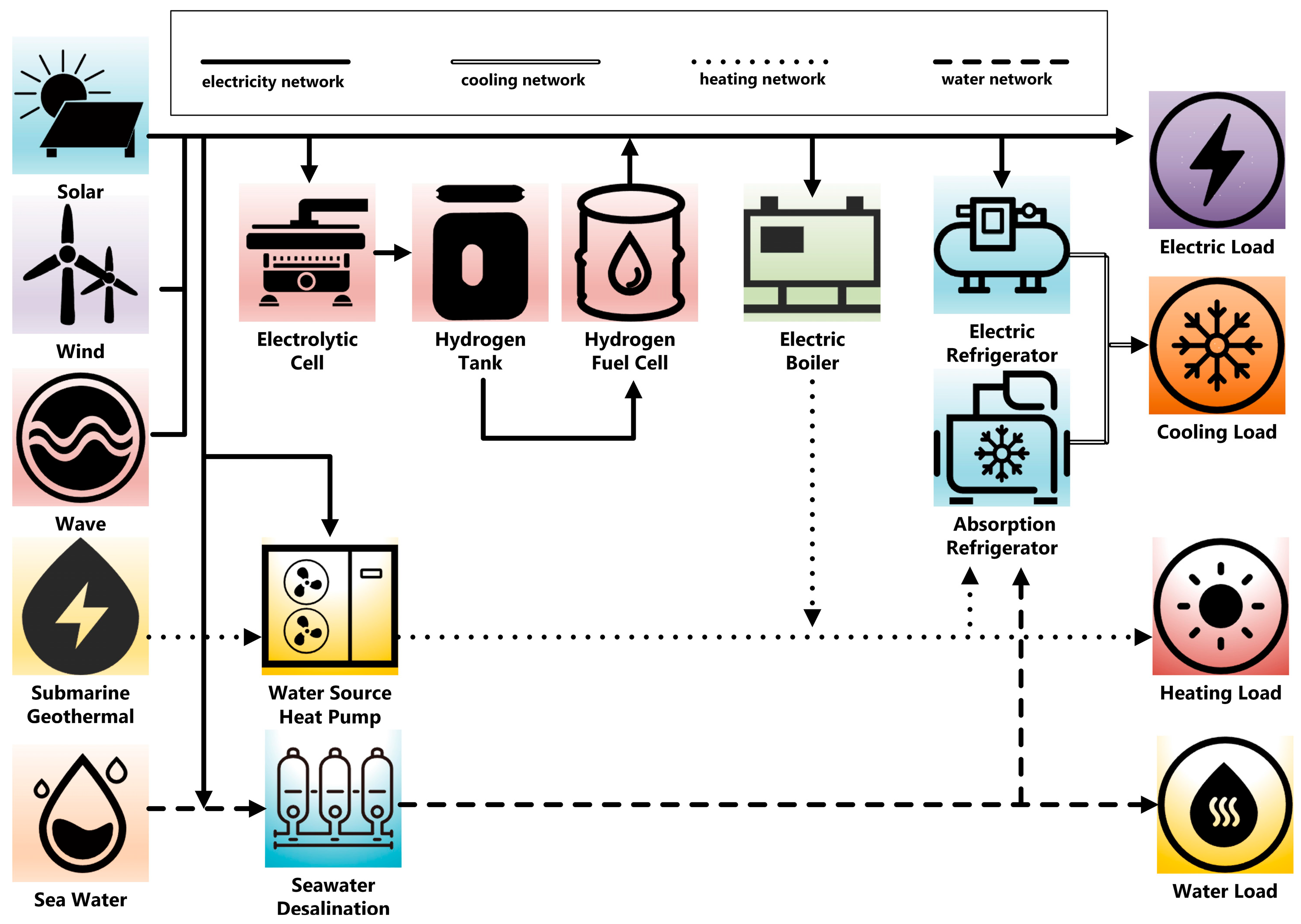
This study conducts a simulation of the integrated energy system for the island depicted in Figure 1, employing a 24 h scheduling period with 1 h dispatch intervals. The Extreme Learning Machine (ELM) [49] method is utilized to generate forecasts based on historical data for wind, solar, and wave energy outputs, as well as daily predictions for electrical, cooling, heating, and water loads over the 24 h scheduling period. As observed in Figure 6, the wind energy output is relatively stable, while solar energy displays significant variability during daylight hours, peaking at midday. Wave energy production is comparatively low, albeit with a slight increase during the evening. Regarding load predictions, electrical demand peaks during the daytime high-demand period, then gradually declines. Cooling and heating loads exhibit a distinct counter-cyclical pattern, with cooling demand peaking during the day and heating demand more pronounced at night. The water load remains relatively stable, with minor fluctuations during certain periods.

We conducted an analysis of wind power output predictions for the integrated energy system on the island, comparing the effects across different confidence intervals ranging from 70% to 98% (as shown in Figure 7). A 95% confidence interval was ultimately selected as the optimal confidence level because it balances forecast accuracy with the avoidance of resource wastage due to overly broad intervals and reduces risks associated with prediction uncertainty [50]. At the 95% confidence level, interval forecasts for various system metrics were performed, with the results displayed in Figure 8, clearly marking the upper and lower bounds of the predicted intervals.

Based on the output data from renewable energy sources and load forecasts, an interval-based multi-objective optimization model for the integrated energy system of islands was solved. The objective functions aimed to minimize daily economic costs and maximize the output from renewable energies. The resulting Pareto frontier is shown in Figure 9.

We conducted a detailed analysis of the energy dispatch performance of an integrated energy system on an island over a 24 h period. As shown in Figure 10, the system dynamically adjusts the output of various energy devices in response to fluctuations in load demand throughout the day, ensuring continuity and diversity of energy supply. During daylight hours, the system fully utilizes solar energy devices for power supply. At night, as solar devices cease to produce energy, the system adjusts the operation of other energy devices, maximizing the output of renewable energy and minimizing costs. This dispatch strategy not only optimizes energy utilization efficiency but also enhances the system’s adaptability to changes in energy demand, further confirming its effectiveness and economic viability in practical applications.

We evaluated the performance of MOMAML-PPO compared to four other algorithms (IP-MOEA, ICMOABC, IMOMA-II, and CIMOEA) within the integrated energy optimization scheduling model for islands. All evolutionary algorithms were tested with a population size of $N=50$ and $Gen=100$ iterations. As shown in

Table 3. Algorithm comparison.

Algorithm Name	Hypervolume	Time/s	Uncertainty
MOMAML-PPO	0.6614	92.4	3.2141
IP-MOEA	0.5785	14,297	22.2541
ICMOABC	0.5436	10,783	28.8451
IMOMA-II	0.5436	14,150	28.4715
CIMOEA	0.5967	1575.5	2.3793

, MOMAML-PPO achieved a hypervolume [51] index of 0.6214, surpassing the other algorithms, indicating its superior capability in exploring the solution space more comprehensively in ICMOPs. Moreover, the computation time of MOMAML-PPO was only 92.4 s, significantly lower than the other algorithms, demonstrating higher time efficiency. The uncertainty of the algorithm is quantified by the mean of the sum of the widths of the objective function intervals for all individuals. Although MOMAML-PPO displayed slightly higher uncertainty compared to CIMOEA, its performance remained within a range of 3.2141. This can be attributed to the fact that the DRL model was designed to address a class of problems rather than a specific experimental case. In contrast, CIMOEA is tailored for direct computation on specific experimental data, resulting in lower uncertainty values than MOMAML-PPO after approximately 80 generations of population evolution, as supported by statistical analysis. Through a lateral comparison between the DRL method and the interval multi-objective evolutionary algorithm, MOMAML has demonstrated outstanding generalization performance. After sufficient training, this algorithm can quickly devise scheduling solutions for different instance scenarios. Not only does MOMAML solve problems faster, meeting the demands of real-time scheduling, but it also shows considerable advantages in the HV index, indicating a higher quality of its solution set.

We investigated the application of the enhanced PPO-CLIP model in the optimization and scheduling systems of comprehensive island energy. The training efficiency and performance of the model were assessed through various parameter initialization strategies. During the experimental design, the model’s weight coefficients were uniformly set at 0.5, and all average reward values were normalized. The number of iterations was fixed at 10,000, processing the same 20 data sets in each iteration to ensure consistency and accuracy in the evaluations.

We performed sensitivity analyses on two pivotal parameters affecting the performance of our model: the learning rate, $\theta$, of the actor–critic network and the discount factor, $\gamma$, for reward computation, as illustrated in Figure 11 and Figure 12. The experiments allocated equal weights of 0.5 to objectives $F_1$ and $F_2$, to ensure the model remained balanced in its pursuit of these distinct goals while pursuing these distinct goals. A total of 5000 iterations were executed, sufficient to evaluate the model’s long-term behavior and stability. The rewards computed in each iteration were normalized.

At a learning rate of $\theta =1.5\times {10}^{-4}$, the model demonstrated both high and stable reward trajectories. When the learning rate was increased to $1.5\times {10}^{-4}$ and further to $1.5\times {10}^{-3}$, the model tended to either overshoot the optimal solution or oscillate around it, resulting in significant reward volatility and challenges in achieving convergence. Conversely, at a lower learning rate of $\theta =1.5\times {10}^{-5}$, the model exhibited greater stability in the final phases, albeit with slower convergence compared to a learning rate of $\theta =1.5\times {10}^{-4}$. Therefore, a learning rate of $\theta =1.5\times {10}^{-4}$ proved optimal, effectively balancing accelerated learning with stability and higher mean rewards.

In Figure 12, we examined the impact of varying discount factors, $\gamma$, on model performance. A setting of $\gamma =0.96$ optimized the balance between immediate and future rewards, enhancing long-term average reward. Higher discount factors, such as $\gamma =0.98$, led the model to over-prioritize long-term rewards, potentially compromising responsiveness to immediate changes. Conversely, lower values of $\gamma$, specifically 0.9 and 0.8, caused an overemphasis on short-term rewards, neglecting long-term strategic development and subsequently diminishing overall performance. Selecting $\gamma =0.96$ facilitated a balance between long-term strategic considerations and immediate responses, thus enhancing the model’s adaptability and robustness across various task environments.

To validate the efficacy of the proposed meta-model parameter initialization strategy, we established one experimental group and two control groups. The control groups were evaluated using domain parameter transfer and random initialization strategies, with each undergoing 10,000 training iterations. The average reward values were normalized for comparison. As depicted in Figure 13, the meta-model parameter transfer strategy (represented by the red line) demonstrated higher average reward values from the early stages of the experiment and reached a stable state after approximately 3500 iterations. This observation suggests that the meta-model parameter transfer strategy significantly enhances the model’s initial performance and accelerates the learning process. Moreover, this strategy not only boosts the model’s rapid adaptability but also enhances its stability and efficiency over long-term iterations.

In comparison, the adjacent sub-model parameter transfer strategy (blue line) initially exhibited lower performance. However, as the iterations progressed, its performance gradually improved, showing comparable results to the meta-model parameter transfer in the mid to late stages of iteration. This indicates that the parameters of adjacent sub-models can gradually adapt and optimize the current model’s performance with sufficient iterations. Compared to the aforementioned strategies, random initialization (green line) showed overall poorer performance, particularly in the initial stages of iteration, highlighting the importance of appropriate parameter initialization in complex system optimization and the challenges that random initialization may pose at the start of model learning. The meta-model parameter transfer method not only improved the training efficiency but also optimized the model’s long-term stability and performance during iterations, confirming the effectiveness of using meta-learning for parameter initialization to enhance model training efficiency.

To assess the resilience of the model under emergent weather conditions, consider two scenarios involving torrential rainfall, which differ in the timing of the rain. In both scenarios, solar power devices are rendered inoperative due to weather constraints, while all wind turbines operate at their maximum rated power of 8 kW. According to the results of the experiment shown in Figure 14, in extreme weather conditions devoid of solar input, wind energy emerges as the primary source of power for the energy system, with a marked increase in output from other devices as well. The power output exhibits significant variability, underscoring the model’s capability to dynamically adjust different devices to meet the continuously changing electricity load demands.

5. Conclusions

This study presents an integrated energy optimization scheduling model for islands based on multi-objective optimization algorithms that account for multiple uncertainties, utilizing a novel approach combining meta-learning with an enhanced PPO-CLIP technique. This method adopts the idea of uniformly decomposed weights from MOEA/D, transforming complex interval multi-objective optimization problems into simpler interval single-objective challenges. By training a meta-model capable of adapting to any weighted subproblem and subsequently fine-tuning it, the model for each subproblem is generated, enabling the solution of all weighted issues. Optimal scheduling solutions are characterized using interval critical points. The conclusions are as follows: (1) MOMAML-PPO inherits the powerful generalization capabilities of DRL, and in scenarios such as the real-time scheduling of integrated energy systems on islands, it can rapidly generate solution sets. (2) The introduction of meta-learning provides robust support for model initialization and parameter tuning, overcoming the traditional drawback of slow training speeds encountered with decomposition methods in DRL. (3) The application of the modified PPO-CLIP algorithm enhances the exploratory capabilities of the system, proving the effectiveness of the action probability “shift” strategy and the GAE method, effectively avoiding potential local optima traps and demonstrating remarkable adaptability to environmental uncertainties. Looking ahead, this research aims to explore more efficient algorithms within the reinforcement learning framework, such as SAC, A3C, and D3QN, to determine if further improvements in model performance and experimental outcomes can be achieved. Through continual technological innovation, this work seeks to provide more precise and reliable theoretical and practical support for the optimization of integrated energy systems on islands.

References

1. Chen, M.F.; Ning, G.T.; Yu, Y.; Miu, S.W.; Fang, B. Research on application of integrated energy planning for island. In Proceedings of the IEEE Conference on Energy Internet and Energy System Integration, Beijing, China, 26–28 November 2017. [Google Scholar] [CrossRef]
2. Lin, J.H.; Wu, Y.K.; Lin, H.J. Successful experience of renewable energy development in several offshore islands. In Proceedings of the International Conference on Power and Energy Systems Engineering, Berlin, Germany, 25–29 September 2017. [Google Scholar] [CrossRef]
3. Tang, H.; Wang, S. A model-based predictive dispatch strategy for unlocking and optimizing the building energy flexibilities of multiple resources in electricity markets of multiple services. Appl. Energy 2022, 305, 117889. [Google Scholar] [CrossRef]
4. Dong, Y.; Zhang, H.; Wang, C.; Zhou, X. Robust optimal scheduling for integrated energy systems based on multi-objective confidence gap decision theory. Expert Syst. Appl. 2023, 228, 120304. [Google Scholar] [CrossRef]
5. Bazmohammadi, N.; Anvari-Moghaddam, A.; Tahsiri, A.; Madary, A.; Vasquez, J.C.; Guerrero, J.M. Stochastic Predictive Energy Management of Multi-Microgrid Systems. Appl. Sci. 2020, 10, 4833. [Google Scholar] [CrossRef]
6. Wang, J.; Zhong, H.; Ma, Z.; Xia, Q.; Kang, C. Review and prospect of integrated demand response in the multi-energy system. Appl. Energy 2017, 202, 772–782. [Google Scholar] [CrossRef]
7. Wang, T.; Han, H.; Wang, Y. A two-stage distributionally robust optimization model for geothermal-hydrogen integrated energy system operation considering multiple uncertainties. Environ. Dev. Sustain. 2024, 26, 16223–16247. [Google Scholar] [CrossRef]
8. Wei, S.R.; Zhang, L.; Xu, Y.; Fu, Y.; Li, F. Hierarchical Optimization for the Double-Sided Ring Structure of the Collector System Planning of Large Offshore Wind Farms. IEEE Trans. Sustain. Energy 2016, 8, 1029–1039. [Google Scholar] [CrossRef]
9. Jia, D.B.; Xu, W.X.; Liu, D.Z.; Xu, Z.X.; Zhong, Z.M.; Ban, X.X. Verification of classification model and dendritic neuron model based on machine learning, Discrete Dyn. Nat. Soc. 2022, 2022, 3259222. [Google Scholar] [CrossRef]
10. Mamani, J.C.M.; Carrasco-Choque, F.; Paredes-Calatayud, E.F.; Cusilayme-Barrantes, H.; Cahuana-Lipa, R. Modeling Uncertainty Energy Price Based on Interval Optimization and Energy Management in the Electrical Grid. Oper. Res. Forum 2023, 5, 4. [Google Scholar] [CrossRef]
11. Jia, D.B.; Li, C.H.; Liu, Q.; Yu, Q.; Meng, X.; Zhong, Z.; Ban, X.; Wang, N. Application and evolution for neuralnetwork and signal processing in large-scale systems. Complexity 2021, 2021, 6618833. [Google Scholar] [CrossRef]
12. Kim, M.; Ham, Y.; Koo, C.; Kim, T.W. Simulating travel paths of construction site workers via deep reinforcement learning considering their spatial cognition and wayfinding behavior. Autom. Constr. 2023, 147, 104715. [Google Scholar] [CrossRef]
13. Jia, D.B.; Dai, H.W.; Takashima, Y.; Nishio, T.; Hirobayashi, K.; Hasegawa, M.; Hirobayashi, S.; Misawa, T. EEG processing in internet of medical things using non-harmonic analysis: Application and evolution for SSVEP responses. IEEE Access 2019, 7, 11318–11327. [Google Scholar] [CrossRef]
14. Wu, Z.; Xiong, Y.; Yu, S.X.; Lin, D. Unsupervised Feature Learning via Non-parametric Instance Discrimination. In Proceedings of the 2018 IEEE/CVF Conference on Computer Vision and Pattern Recognition, Salt Lake City, UT, USA, 18–23 June 2018; pp. 3733–3742. [Google Scholar] [CrossRef]
15. Wu, Z.T.; Dijkstra, P.; Koch, G.W.; Peñuelas, J.; Hungate, B.A. Responses of terrestrial ecosystems to temperature and precipitation change: A meta-analysis of experimental manipulation. Glob. Change Biol. 2011, 17, 927–942. [Google Scholar] [CrossRef]
16. Gao, S.C.; Yu, Y.; Wang, Y.R.; Wang, J.H.; Cheng, J.J.; Zhou, M.C. Chaotic Local Search-based Differential Evolution Algorithms for Optimization. IEEE Trans. Syst. Man Cybern. Syst. 2021, 51, 3954–3967. [Google Scholar] [CrossRef]
17. Chen, Z.W.; Chen, L.; Bai, X.; Yang, Q.; Zhao, F.L. Interactive multi-attribute decision-making NSGA-II for constrained multi-objective optimization with interval numbers. Control. Decis. 2015, 30, 865–870. [Google Scholar]
18. Zeng, B.; Zhang, W.X.; Hu, P.D.; Sun, J.; Gong, D. Synergetic renewable generation allocation and 5G base station placement for decarbonizing development of power distribution system: A multi-objective interval evolutionary optimization approach. Appl. Energy 2023, 351, 121831. [Google Scholar] [CrossRef]
19. Jia, D.B.; Yanagisawa, K.; Ono, Y.; Hirobayashi, K.; Hasegawa, M.; Hirobayashi, S.; Tagoshi, H.; Narikawa, T.; Uchikata, N.; Takahashi, H. Multiwindow nonharmonic analysis method for gravitational waves. IEEE Access 2018, 6, 48645–48655. [Google Scholar] [CrossRef]
20. Jia, D.B.; Yanagisawa, K.; Hasegawa, M.; Hirobayashi, S.; Tagoshi, H.; Narikawa, T.; Uchikata, N. Timefrequency based non-harmonic analysis to reduce line noise impact for LIGO observation system. Astron 2018, 25, 238–246. [Google Scholar]
21. Yu, Q.; Yang, C.; Dai, G.; Peng, L.; Li, J. A novel penalty function-based interval constrained multi-objective optimization algorithm for uncertain problems. Swarm Evol. Comput. 2024, 88, 101584. [Google Scholar] [CrossRef]
22. Ming, F.; Gong, W.; Wang, L.; Jin, Y. Constrained Multi-Objective Optimization with Deep Reinforcement Learning Assisted Operator Selection. IEEE/CAA J. Autom. 2024, 11, 919–931. [Google Scholar] [CrossRef]
23. Jia, D.B.; Fujishita, Y.; Li, C.H.; Todo, Y.; Dai, H.W. Validation of large-scale classification problem in dendritic neuron model using particle antagonism mechanism. Electronics 2020, 9, 792. [Google Scholar] [CrossRef]
24. Huang, N.C.; Hsieh, P.C.; Ho, K.H.; Wu, I.C. PPO-Clip Attains Global Optimality: Towards Deeper Understandings of Clip. In Proceedings of the AAAI Conference on Artificial Intelligence, Vancouver, BC, Canada, 20–28 February 2024; Volume 38, pp. 12600–12607. [Google Scholar]
25. Zhang, Z.; Wu, Z.; Wang, J. Meta-Learning-based Deep Reinforcement Learning for Multi-objective Optimization Problems. IEEE Trans. Neural Netw. Learn. Syst. 2022, 34, 7978–7991. [Google Scholar] [CrossRef]
26. Hu, Q. Application of Fuzzy Uncertainty Optimization Theory in Energy Planning; North China Electric Power University: Beijing, China, 2013. [Google Scholar]
27. Bai, L.Q.; Li, F.; Cui, H.; Jiang, T.; Sun, H.; Zhu, J. Interval optimization based operating strategy for gas-electricity integrated energy systems considering demand response and wind uncertainty. Appl. Energy 2016, 167, 270–279. [Google Scholar] [CrossRef]
28. Zhang, C.; Chen, H.Y.; Liang, Z.P.; Mo, W.; Zheng, X.; Hua, D. Interval voltage control method for transmission systems considering interval uncertainties of renewable power generation and load demand. IET Gener. Transm. Distrib. 2018, 12, 4016–4025. [Google Scholar] [CrossRef]
29. Li, P.; Yu, D.; Yang, M.; Wang, J. Flexible look-ahead dispatch realized by robust optimization considering CVAR of wind power. IEEE Trans. Power Syst. 2018, 33, 5330–5340. [Google Scholar] [CrossRef]
30. Wang, Y.; Wang, Y.; Huang, Y.; Yang, J.; Ma, Y.; Yu, H.; Zeng, M.; Zhang, F.; Zhang, Y. Operation optimization of regional integrated energy system based on the modeling of electricity-thermal-natural gas network. Appl. Energy 2019, 251, 113410. [Google Scholar] [CrossRef]
31. Yan, L.; Chen, X.; Zhou, J.; Chen, Y.; Wen, J. Deep reinforcement learning for continuous electric vehicles charging control with dynamic user behaviors. IEEE Trans. Smart Grid 2021, 12, 5124–5134. [Google Scholar] [CrossRef]
32. Zheng, L.; Wu, H.; Guo, S.; Sun, X. Real-time dispatch of an integrated energy system based on multi-stage reinforcement learning with an improved action-choosing strategy. Energy 2023, 277, 127636. [Google Scholar] [CrossRef]
33. Wang, J.J.; Zhao, L.; Lu, H.; Wei, C. Multi-objective stochastic-robust based selection-allocation-operation cooperative optimization of rural integrated energy systems considering supply-demand multiple uncertainties. Renew. Energy 2024, 233, 121159. [Google Scholar] [CrossRef]
34. Li, Y.; Bu, F.; Li, Y.; Long, C. Optimal scheduling of island integrated energy systems considering multi-uncertainties and hydrothermal simultaneous transmission: A deep reinforcement learning approach. Appl. Energy 2023, 333, 120540. [Google Scholar] [CrossRef]
35. Ren, H.B.; Jiang, Z.; Wu, Q.; Li, Q.; Lv, H. Optimal planning of an economic and resilient district integrated energy system considering renewable energy uncertainty and demand response under natural disasters. Energy 2023, 277, 127644. [Google Scholar] [CrossRef]
36. Brewer, B.C.; Bantis, L.E. Cutoff estimation and construction of their confidence intervals for continuous biomarkers under ternary umbrella and tree stochastic ordering settings. Stat. Med. 2024, 43, 606–623. [Google Scholar] [CrossRef]
37. Gao, S.C.; Zhou, M.C.; Wang, Z.Q.; Sugiyama, D.; Cheng, J.J.; Wang, J.H.; Todo, Y.K. Fully Complex-valued Dendritic Neuron Model. IEEE Trans. Neural Netw. Learn. Syst. 2023, 34, 2105–2118. [Google Scholar] [CrossRef] [PubMed]
38. Jia, D.B.; Xu, Z.X.; Wang, Y.C.; Ma, R.; Jiang, W.Z.; Qian, Y.L.; Wang, Q.J.; Xu, W.X. Application of intelligent time series prediction method to dew point forecast. Electron. Res. Arch. 2023, 31, 2878–2899. [Google Scholar] [CrossRef]
39. Hao, Z.W.; Zhou, J.; Lin, S.; Lan, D.; Li, H.; Wang, H.; Liu, D.; Gu, J.; Wang, X.; Wu, G. Customized heterostructure of transition metal carbides as high-efficiency and anti-corrosion electromagnetic absorbers. Carbon 2024, 228, 119323. [Google Scholar] [CrossRef]
40. Ramirez-Atencia, C.; Mostaghim, S.; Camacho, D. KPNSGA-II: Knee point based MOEA with self-adaptive angle for Mission Planning Problems. arXiv 2020, arXiv:2002.08867. [Google Scholar] [CrossRef]
41. Wu, X.; Zhang, K. A penalty function-based greedy diffusion search algorithm for the optimization of constrained nonlinear dynamical processes with discrete-valued input. J. Ind. Manag. Optim. 2023, 19, 6856–6885. [Google Scholar] [CrossRef]
42. Schulman, J.; Moritz, P.; Levine, S.; Jordan, M.; Abbeel, P. High-Dimensional Continuous Control Using Generalized Advantage Estimation. arXiv 2015, arXiv:1506.02438. [Google Scholar] [CrossRef]
43. Sun, J.; Miao, Z.; Gong, D.W.; Zeng, X.J.; Li, J.Q.; Wang, G.G. Interval Multi-objective Optimization with Memetic Algorithms. IEEE Trans. Cybern. 2020, 50, 3444–3457. [Google Scholar] [CrossRef] [PubMed]
44. Philipp, L.; Salazar, A.D.E. An optimization algorithm for imprecise multi-objective problem functions. IEEE Congr. Evol. Comput. 2005, 1, 459–466. [Google Scholar]
45. Zhang, L.M.; Wang, S.S.; Zhang, K.; Zhang, X.Q.; Sun, Z.X.; Zhang, H.; Chipecane, M.T.; Yao, J. Cooperative artificial bee colony algorithm with multiple populations for interval multiobjective optimization problems. IEEE Trans. Fuzzy Syst. 2019, 27, 1052–1065. [Google Scholar] [CrossRef]
46. Wang, F.M.; Sun, J.; Gan, X.J.; Dai, H.W.; Dai, Y.C. An Interval Multi-Objective Optimization Strategy of Island Integrated Energy System Considering Multiple Uncertainties. ICIC Express Lett. 2023, 17, 1143. [Google Scholar]
47. Xu, W.X.; Jia, D.B.; Zhong, Z.M.; Li, C.; Xu, Z. Intelligent dendritic neural model for classification problems. Symmetry 2022, 14, 11. [Google Scholar] [CrossRef]
48. Gao, Z.G.; Lan, D.; Ren, X.; Jia, Z.; Wu, G. Manipulating cellulose-based dual-network coordination for enhanced electromagnetic wave absorption in magnetic porous carbon nanocomposites. Compos. Commun. 2024, 48, 101922. [Google Scholar] [CrossRef]
49. Wang, J.; Lu, S.; Wang, S.H.; Zhang, Y.D. A review on extreme learning machine. Multimed. Tools Appl. 2022, 81, 41611–41660. [Google Scholar] [CrossRef]
50. Lan, D.X.; Hu, Y.; Wang, M.; Wang, Y.; Gao, Z.; Jia, Z. Perspective of electromagnetic wave absorbing materials with continuously tunable effective absorption frequency bands. Compos. Commun. 2024, 50, 101993. [Google Scholar] [CrossRef]
51. Deveci, K.; Guler, O. Ranking intuitionistic fuzzy sets with hypervolume-based approach: An application for multi-criteria assessment of energy alternatives. Appl. Soft Comput. 2024, 150, 111038. [Google Scholar] [CrossRef]
Figure 1. IIES architecture.
Electronics 13 03579 g001
Figure 2. MOMAML-PPO solution process.
Electronics 13 03579 g002
Figure 3. Solution selection at interval knee points.
Electronics 13 03579 g003
Figure 4. Meta-learning training.
Electronics 13 03579 g004
Figure 5. Schematic of the enhanced PPO-CLIP method.
Electronics 13 03579 g005
Figure 6. Forecasting renewable energy output and multiple load demands.
Electronics 13 03579 g006
Figure 7. Comparison of wind power output intervals under different confidence levels.
Electronics 13 03579 g007
Figure 8. The 95% confidence interval forecasting for renewable energy output and load demands.
Electronics 13 03579 g008
Figure 9. Pareto frontier of the ICMOP solution. (a) Pareto front boundary point plot; (b) Pareto front matrix plot.
Electronics 13 03579 g009
Figure 10. Scheduling results.
Electronics 13 03579 g010
Figure 11. Sensitivity analysis of the learning rate parameter in actor–critic networks.
Electronics 13 03579 g011
Figure 12. Sensitivity analysis of the reward discount factor in coefficient parameters.
Electronics 13 03579 g012
Figure 13. Average reward change curve.
Electronics 13 03579 g013
Figure 14. Dispatch strategy under emergency conditions: (a) scheduling results for Emergent Scenario 1; (b) scheduling results for Emergent Scenario 2.
Electronics 13 03579 g014