A Novel Areal Maintenance Strategy for Large-Scale Distributed Photovoltaic Maintenance

Abstract

A smart grid is designed to enable the massive deployment and efficient use of distributed energy resources, including distributed photovoltaics (DPV). Due to the large number, wide distribution, and insufficient monitoring information of DPV stations, the pressure to maintain them has increased rapidly. Furthermore, based on reports in the relevant literature, there is still a lack of efficient large-scale maintenance strategies for DPV stations at present, leading to the high maintenance costs and overall low efficiency of DPV stations. Therefore, this paper proposes a maintenance period decision model and an areal maintenance strategy. The implementation steps of the method are as follows: firstly, based on the reliability model and dust accumulation model of the DPV components, the maintenance period decision model is established for different numbers of DPV stations and different driving distances; secondly, the optimal maintenance period is determined by using the Monte Carlo method to calculate the average economic benefits of daily maintenance during different periods; then, an areal maintenance strategy is proposed to classify all the DPV stations into different areas optimally, where each area is maintained to reach the overall economic optimum for the DPV stations; finally, the validity and rationality of this strategy are verified with the case study of the DPV poverty alleviation project in Badong County, Hubei Province. The results indicate that compared with an independent maintenance strategy, the proposed strategy can decrease the maintenance cost by 10.38% per year, which will help promote the construction of the smart grid and the development of sustainable cities. The results prove that the method proposed in this paper can effectively reduce maintenance costs and improve maintenance efficiency.

1. Introduction

With non-renewable energy sources almost on the verge of depletion, it is essential to derive energy from renewable sources for the benefit of humankind. Due to the advantages of having low carbon emissions, being environmental friendly, being rich in resources, and having strong adaptability to local conditions, distributed photovoltaics (DPV) is increasingly contributing to promoting the energy transformation and sustainable economic development [1,2]. According to the statistics from the National Energy Administration, the cumulative installed capacity of DPV in China had exceeded 254.4 GW by the end of 2023, and the new installed capacity that year exceeded 96.2 GW [3]. DPV capacity is predicted to maintain rapid growth in the future, based on the implementation of China’s national strategies of carbon peaking and the goals of carbon neutrality and rural revitalization [4,5].

With the rapid development of DPV, maintenance technology plays a vital role in improving the reliability and energy utilization of DPV. Also, reasonable maintenance can effectively improve the profitability of DPV and reduce the unit price of power generation [6,7]. In traditional large-scale centralized PV stations, there are generally maintainers on duty and regular operation and maintenance procedures [8], while DPV stations are numerous, widely distributed, and designed not to have to be attended to [9]. Moreover, DPV stations lack effective state monitoring, and a very significant proportion of DPV stations has even been installed without any monitoring [10]. At present, most DPV stations still follow the maintenance strategy of traditional PV stations for regular maintenance, and the maintenance period is mainly determined by practical experience. In addition, since one maintainer is typically in charge of one DPV, the large-scale maintenance of DPV stations lacks an overall strategy, resulting in high maintenance costs and low power generation efficiency [11,12]. Thus, how to create a reasonable DPV station maintenance strategy to ensure its power generation efficiency and reduce maintenance costs as much as possible has become a key problem to be solved.

The maintenance of PV fault equipment is a major part of PV maintenance. Research on the reliability of PV is mainly divided into two types of reliability models: one is based on component failure, and the other is based on resource constraints [13]. The main research methods include reliability block diagrams [14], fault tree analysis [15], and the Markov method [16]. PV module cleaning is another major part of PV maintenance. PV stations tend to be exposed to the environment for a long time, and tiny particles in the air are easily deposited on the module panels and eventually form a dust layer, which reduces the light transmittance and power generation of the module [17]. Darwish et al. [18] tracked the dust accumulation on PV systems, and within one month, the dust accumulation density increased by 5.44 g/${\mathrm{m}}^2$, while the power generation decreased by 12.7%. Zaihidee et al. [19] conducted indoor dust accumulation experiments by using dust emitters and fans, and the results showed that the dust accumulation caused by different environments, installation inclination angles, and dust types reduced the power generation by about 15–35% when its density reached 20 g/${\mathrm{m}}^2$.

Several studies have been conducted on PV maintenance. Reference [12] investigated the maintenance methods and prices of PVs in the United States. The results showed that the budgets for maintenance are quite different, and there is still a lack of a mature DPV maintenance method. Reference [20] analyzed the impact of different types of maintenance contracts on the economy of DPV stations, taking Spain’s DPV stations as an example. The results showed that for small and medium DPV stations (≤100 kW), it is more profitable to retain only corrective maintenance and forgo preventive maintenance. Reference [21] divides the PV maintenance modes into four types: PV owner maintenance, PV manufacturer maintenance, third-party maintenance, and areal cooperative maintenance. The author took into account the indicators of professionalism, timeliness, and economics and then used the fuzzy analytical hierarchy process to determine the maintenance mode. Reference [22] designed a distributed home PV maintenance structure, which optimizes the total maintenance cost under the condition of comprehensively optimizing the location of the maintenance company and the number of maintainers in the company. Reference [23] evaluated the different failure risks of PV systems in three aspects: severity, occurrence, and detection. The authors proposed to reduce the failure risk of PV systems by installing overload-measuring equipment and thermal imagers. Reference [24] analyzed the influence of temperature and exposure time on the dust deposition rate of PV modules. The authors established a multiple linear regression model and a neural network model that predicted the value of the dependent variables with multiple independent variables to evaluate the daily dust deposition rate and analyzed the effectiveness of the model by using Jordanian data. Based on the evaluation model, recommendations for PV module cleaning times were given.

However, there is still a lack of research on DPV maintenance period optimization considering both component reliability and dust accumulation. Research on the large-scale areal maintenance strategies for DPV stations is also insufficient, resulting in unreasonable maintenance and low economic efficiency for DPV stations.

To address this issue, this paper introduces a DPV maintenance period decision model. This model takes into account both power generation losses and maintenance costs. The Monte Carlo method is employed to calculate the optimal maintenance period and the associated optimal economic benefits, considering varying numbers of DPV stations and driving distances. On this basis, a large-scale areal maintenance strategy for DPV stations is proposed. This strategy aims to optimally classify all stations into distinct areas, with each area being maintained as a unit according to its own optimal maintenance period. The proposed strategy can reduce the total maintenance cost and improve the overall profitability of DPV stations.

Section 1 provides an overview of the research background, current status, and existing limitations in the field. Section 2 provides an overview, the structure, and the implementation of the maintenance period decision model. Section 3 introduces the areal maintenance strategy, including its overview, model construction, and proposed solutions. Section 4 presents the model parameters, such as DPV station structure, failure rate, dust accumulation rate, and economic parameters. Section 5 presents the results of the maintenance period decision model and the areal maintenance strategy. Finally, Section 6 concludes the study and outlines potential avenues for further investigation.

2. Maintenance Period Decision Model

The maintenance period decision model aims to find the optimal maintenance period to obtain the best maintenance economic benefits for the designated DPV stations. The input parameters of the model are the candidate solutions of the maintenance period, and the output parameters are the optimal maintenance period and the maintenance economic benefits. The maintenance period decision model is obtained by combining the reliability model and the dust accumulation model, where the reliability model is obtained by describing the failure time of the component by the probability function, while the relationship between dust density and power generation loss is obtained with the dust accumulation model.

2.1. Model Overview

The maintenance period decision model aims to determine the optimal maintenance period to obtain the best maintenance economic benefits for the designated DPV stations. The input parameters of the model are the candidate solutions of the maintenance period, and the output parameters are the optimal maintenance period and the maintenance economic benefits.

PV maintenance involves two key components: fault component repair and module cleaning. The maintenance economic benefits are mainly composed of two parts. One is the power generation loss cost due to the failure of components or the dust on the modules, and the other is the maintenance cost. If the maintenance period becomes too long, the fault components grow in number, the failure time expands, and the accumulation of dust on the modules also increases. All of these make PV power generation lower than expected, decreasing the economic benefits. Conversely, if the maintenance period becomes too short, the annual maintenance times grow, and the maintenance cost is too high, even exceeding the power generation loss cost. Thus, this paper seeks to find a balance between the power generation loss cost and the maintenance cost to achieve the optimal maintenance economic benefits.

Given the random nature of component failures, the power generation loss cost and the maintenance cost in each maintenance period are distinct. To address this, we establish a component reliability model and use the Monte Carlo method to obtain the probability distribution of the model results. Additionally, due to the increase in dust accumulation over operating time, the blocking effect on light leads to a loss of power of the PV; thus, we develop a dust accumulation model to quantify the power loss caused by it.

2.2. PV Component Reliability Model and Dust Accumulation Model

The failure rate $\lambda$ can be defined as the anticipated time at which an item fails in a specified period of time [25]. The value of $\lambda$ changes in the life cycle of the item. The bathtub curve refers to the change in the reliability of the product from the time it is put into production to the end of life. A typical bathtub curve which represents the failure pattern is shown in Figure 1. The bathtub curve is divided into three stages: early failure, useful life, and wear-out. This paper only considers the maintenance in the useful life where the PVs stay stable operation, that is, $\lambda$ remains unchanged.

The definition of reliability is the ability of a component to complete its specified tasks without failure within a specified time under specific environmental and operating conditions [26]. In reliability modeling, the failure time of an item is treated as a random variable, which can be described by using various probability functions. The probability density function $f\left(t\right)$ refers to the relative probability of a random variable taking a specific value. The probability of a component failure before a certain time t can be expressed by the cumulative density function $F\left(t\right)$. The relationship between $F\left(t\right)$ and $f\left(t\right)$ is as follows:

$$\begin{array}{c}\hfill \begin{array}{c}\hfill F\left(t\right)={\int }_0^{t}f\left(t\right)dt\end{array}\end{array}$$

(1)

The reliability function represents the probability that the system will not fail within time (0–t]:

$$\begin{array}{c}\hfill \begin{array}{c}\hfill R\left(t\right)=1-F\left(t\right)={\int }_t^{\infty }f\left(t\right)\end{array}\end{array}$$

(2)

The probability density function of component failure of DPV generally adopts an exponential distribution [27]:

$$\begin{array}{c}\hfill \begin{array}{c}\hfill f\left(t\right)=\lambda ·exp(-\lambda t)\end{array}\end{array}$$

(3)

$$\begin{array}{c}\hfill \begin{array}{c}\hfill F\left(t\right)=1-exp(-\lambda t)\end{array}\end{array}$$

(4)

$$\begin{array}{c}\hfill \begin{array}{c}\hfill R\left(t\right)=exp(-\lambda t)\end{array}\end{array}$$

(5)

Due to environmental exposure, various types of dust inevitably accumulate on the surface of the PV modules. The accumulation of dust blocks, absorbs, and reflects light and reduces the light transmittance of the module, bringing about a decrease in power generation under the same meteorological conditions. Consequently, the accumulation of dust on PV modules is also such a vital cause of power generation loss of PV stations that it is necessary to perform module cleaning during maintenance.

Existing research on PV dust accumulation mainly focuses on the relationship between dust accumulation density and power generation loss. There are still few studies on the dust accumulation rate. This paper refers to the dust accumulation model in [28], and the model is as follows:

$$\begin{array}{c}\hfill \begin{array}{c}\hfill {\eta }_{\mathrm{ash}}\left(d\right)=a·(1-exp(b·d))\times 100\%\end{array}\end{array}$$

(6)

where d represents the d day after the modules are completely cleaned; ${\eta }_{\mathrm{ash}}\left(d\right)$ is the power generation loss rate caused by dust on the d day; and a and b are empirical constants, which are determined by the environment in which the PV station is located.

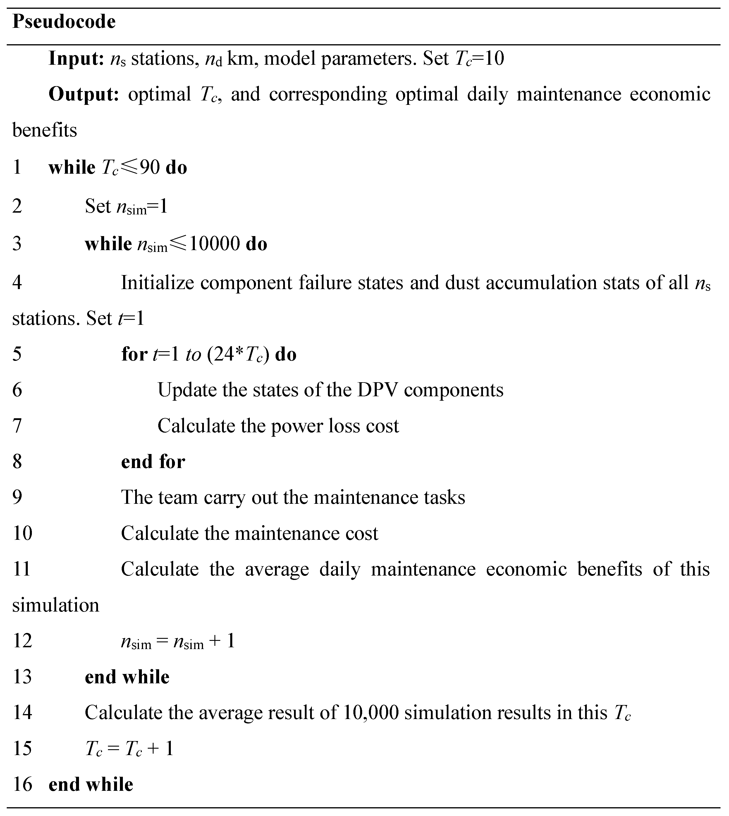
2.3. Model Implementation

This paper uses Matlab to establish the DPV maintenance period decision model and simulates the candidates of the maintenance periods $T_{\mathrm{c}}$ = [10, 90] days. Due to the random failure of PV components obtained through Equations (1)–(6), it is not conducive to universality to run the model only once. Therefore, we use the Monte Carlo method to run the model 10,000 times for each maintenance period to obtain its total economic benefit probability distribution and finally obtain the optimal maintenance period through the mean value of 10,000 simulations.

The model is simulated for $T_{\mathrm{c}}$ days each time, the operation step is 1 h, and t indicates that the model runs at the t-th hour. It is assumed that there are $n_s$ DPV stations that need to be maintained together. The structures of all $n_s$ stations are consistent and independent of each other. That means that the failure of one station does not affect the operation of the other stations.

Once the model simulation starts, the state of the DPV components changes as the simulation goes on. Each component has 4 states. The first one is the normal state, in which DPV modules are connected to the grid to generate electricity, and the amount of dust on the modules continues to increase. The second one is the failure state. When a PV module fails, even if the fault is unrepaired, the inverter can continue operating as long as the PV array reaches the minimum operating voltage required by the inverter [29]. However, once the inverter fails, the power generated by its connected modules cannot be sent to the grid, which is equivalent to the modules being off-grid. Accordingly, it is assumed in this paper that the failure of modules does not affect the operation of other components, while the failure of other components causes the off-grid and zero-power generation of all modules connected to them. And the failure time of the component is randomly determined by the reliability model. The third one is the repair state, in which the components are still invalid and return to the normal state after the repair is completed. The fourth one is the cleaning state. Since the cleaning time of each module is very short, it is unable to accurately evaluate the power generation loss caused by dust in this state. Therefore, we assume that the ${\eta }_{\mathrm{ash}}$ of all DPV modules is half of that at the beginning of cleaning during the cleaning time and becomes 0 again after cleaning.

Once the predetermined maintenance period is reached, a maintenance team is dispatched to service all $n_s$ stations. The team perform four distinct actions. First, they travel from the maintenance company to each station and complete the necessary maintenance tasks, before returning to the company. Second, they engage in a sequence of opening and closing procedures. Upon arriving at a station, the team shut down all components connected to the failed component within the relevant branch. After repair, they reopen all components. This action is assumed to be instantaneous and cost-free. Third, the team repair the failed components by using appropriate maintenance tools and a sufficient supply of spare parts. Finally, after completing all repairs at a station, the team proceed to clean all the modules. During this cleaning process, all modules are considered to be in a cleaning state. Once cleaning is finished, the team proceed to the next station.

The pseudocode of the model implementation is shown in Figure 2.

2.4. Maintenance Economic Benefits

2.4.1. Power Generation Loss Cost

The power generation loss cost is mainly composed of two parts: the loss cost caused by failed components and the cost caused by module dust.

(a) Loss cost caused by failed components

The loss cost caused by failed components is expressed as

$$\begin{array}{c}\hfill \begin{array}{c}\hfill C_{\mathrm{fai},i}\left(t\right)=N_{\mathrm{fm},i}\left(t\right)P\left(t\right)p_{\mathrm{el}}\end{array}\end{array}$$

(7)

$$\begin{array}{c}\hfill \begin{array}{c}\hfill C_{\mathrm{fai}}\left(t\right)=\sum _{i=1}^{n_s}{C}_{\mathrm{fai},i}\left(t\right)\end{array}\end{array}$$

(8)

where $C_{\mathrm{fai}}\left(t\right)$ represents the loss cost caused by component failure at time t; $C_{\mathrm{fai},i}\left(t\right)$ represents the loss cost of the i-th station; $N_{\mathrm{fm},i}\left(t\right)$ represents the total number of offline DPV modules; $P\left(t\right)$ represents the output power of a single module at time t; and $p_{\mathrm{el}}$ is the grid-connected electricity price.

The failure of the components makes all the connected modules offline. $N_{\mathrm{fm},i}\left(t\right)$ is expressed as

$$\begin{array}{c}\hfill \begin{array}{c}\hfill N_{\mathrm{fm},i}\left(t\right)=\sum _j{n}_{\mathrm{fc},j,i}\left(t\right)n_{\mathrm{con},j}\end{array}\end{array}$$

(9)

where $n_{\mathrm{fc},j,i}\left(t\right)$ represents the total number of j-th components that fail at time t. $n_{\mathrm{con},j}$ represents the number of modules connected to the j-th component.

(b) Loss cost caused by module dust

The loss cost caused by module dust is expressed as

$$\begin{array}{c}\hfill \begin{array}{c}\hfill C_{\mathrm{dust},i}\left(t\right)=\left(N_{\mathrm{tol}}-N_{\mathrm{fm},i}\left(t\right)\right)P\left(t\right){\eta }_{\mathrm{ash}}\left(t\right)p_{\mathrm{el}}\end{array}\end{array}$$

(10)

$$\begin{array}{c}\hfill \begin{array}{c}\hfill C_{\mathrm{dust}}\left(t\right)=\sum _{i=1}^{n_s}{C}_{\mathrm{dust},i}\left(t\right)\end{array}\end{array}$$

(11)

where $C_{\mathrm{dust}}\left(t\right)$ represents the loss cost caused by module dust at time t; $C_{\mathrm{dust},i}\left(t\right)$ represents the loss cost of the i-th station; $N_{\mathrm{tol}}$ represents the total number of modules in one station. $\left(N_{\mathrm{tol}}-N_{\mathrm{fm},i}\left(t\right)\right)$ represents the total number of online modules at time t.

2.4.2. Maintenance Cost

(a) Vehicle fuel cost

$$\begin{array}{c}\hfill \begin{array}{c}\hfill C_{\mathrm{vel}}=n_{\mathrm{d}}·c_{\mathrm{vel}}\end{array}\end{array}$$

(12)

where $n_{\mathrm{d}}$ represents the total driving distance of the maintenance team, in km, and $c_{\mathrm{vel}}$ represents the fuel cost per kilometer.

(b) Cleaning cost

$$\begin{array}{c}\hfill \begin{array}{c}\hfill C_{\mathrm{cl}}=n_s·c_{\mathrm{cl}}\end{array}\end{array}$$

(13)

where $c_{\mathrm{cl}}$ represents the cleaning cost of one station. Cleaning cost refers to the cost of cleaning the dust on the PV panels, including water and cleaning agent costs.

(c) Base salary for maintainers

$$\begin{array}{c}\hfill \begin{array}{c}\hfill C_{\mathrm{bs}}=n_{\mathrm{p}}·c_{\mathrm{bs}}\end{array}\end{array}$$

(14)

where $c_{\mathrm{bs}}$ represents the daily base salary for each maintainer. $n_{\mathrm{p}}$ represents the number of maintainers in the maintenance team. The expression of $n_{\mathrm{p}}$ is as follows:

$$\begin{array}{c}\hfill \begin{array}{c}\hfill n_{\mathrm{p}}={\displaystyle \frac{N_{\mathrm{f}}\left(T\right)·t_{\mathrm{fix}}+n_s·t_{\mathrm{cl}}}{wl-n_{\mathrm{d}}/v}}\end{array}\end{array}$$

(15)

where $N_{\mathrm{f}}\left(T\right)$ represents the total number of components that fail in the maintenance period T of all $n_s$ stations. $t_{\mathrm{fix}}$ represents the time spent fixing each failed component. This paper assumes that the time consumption for fixing each component is the same; $t_{\mathrm{cl}}$ represents the time spent cleaning the dust at one station; $wl$ represents the maximum working time of a maintainer for a day; v represents the driving speed.

(d) Workload salary for maintainers

$$\begin{array}{c}\hfill \begin{array}{c}\hfill C_{\mathrm{w}}=(N_{\mathrm{f}}\left(T\right)·t_{\mathrm{fix}}+n_s·t_{\mathrm{cl}})·c_{\mathrm{w}}\end{array}\end{array}$$

(16)

where $c_{\mathrm{w}}$ represents the hourly wage for the maintainers.

2.4.3. Total Economic Benefits

According to Equations (7)–(16), the total economic benefits in a maintenance period can be obtained by adding together the power generation loss cost and the maintenance cost:

$$\begin{array}{c}\hfill \begin{array}{c}\hfill C_{\mathrm{tol}}=\sum _{t=1}^{t_{\mathrm{tol}}}[C_{\mathrm{fai}}\left(t\right)+C_{\mathrm{dust}}\left(t\right)]+C_{\mathrm{vel}}+C_{\mathrm{bs}}+C_{\mathrm{pd}}+C_{\mathrm{w}}\end{array}\end{array}$$

(17)

Then, the average daily maintenance economic benefits are given as

$$\begin{array}{c}\hfill \begin{array}{c}\hfill C_{\mathrm{mean}}={\displaystyle \frac{C_{\mathrm{tol}}}{T_{\mathrm{c}}}}\end{array}\end{array}$$

(18)

3. Areal Maintenance Strategy

3.1. Strategy Overview

Currently, DPV stations typically employ an independent maintenance mode, where each DPV is serviced separately at predetermined intervals. This approach has two significant drawbacks: First, maintainers must travel from the maintenance center to each DPV individually, resulting in wasted travel time and distance. Second, this approach necessitates longer work periods for maintainers, leading to increased base salary costs. Consequently, the independent maintenance mode suffers from low resource utilization and high maintenance costs, hindering the overall economic viability of DPV systems. To address these issues, this paper proposes an areal maintenance strategy for DPV.

By analyzing the optimal maintenance period model of a single station established in Section 2, $C_{\mathrm{fai}}$, $C_{\mathrm{dust}}$, $C_{\mathrm{cl}}$, and $C_{\mathrm{w}}$ increase as the number of DPV stations increases; $C_{\mathrm{vel}}$ increases with the maintenance driving distance; and $C_{\mathrm{bs}}$ is positively correlated with the number of maintenance PV stations and the driving distance. Hence, it is clear that the optimal maintenance period and maintenance economic benefits depend on the number of DPV stations and the driving distance, which can be obtained by classifying the DPV stations into different areas.

Therefore, the areal maintenance strategy can be modeled as a DPV station classification problem to determine the specific stations in each area. In this way, the optimal maintenance period and maintenance economic benefits of each area can be determined, so as to achieve the overall optimal maintenance benefit of DPV.

Considering real-world conditions, our model obeys the following assumptions:

(1) The distance between the maintenance center and DPV stations, as well as between any two DPV stations, is measured as a straight-line distance.

(2) Each maintenance area utilizes one vehicle, with an unlimited number of vehicles and unlimited vehicle capacity.

(3) All maintainers possess common maintenance skills.

(4) All maintainers return to the O&M center at the end of the day.

3.2. Model Construction

3.2.1. Objective Function

This paper calculates the optimal maintenance period and economic benefits for different numbers of DPV stations and different driving distances (the number of stations is incremented by 1, and the driving distance is incremented by 1 km). They are denoted by $S_{\mathrm{per}}\left(n_{\mathrm{s}},n_{\mathrm{d}}\right)$ and $S_{\mathrm{ben}}\left(n_{\mathrm{s}},n_{\mathrm{d}}\right)$, respectively. $n_{\mathrm{s}}$ and $n_{\mathrm{d}}$ represent the number of stations and the driving distance of the area, respectively.

The total number of DPV stations is set to $N_{\mathrm{s}}$, each station is expressed as $x_j(j=1,2,\dots ,N_{\mathrm{s}})$, and the total number of areas is set to $N_{\mathrm{R}}$. Then, this paper assigns an areal number to each station, $x_j\in [1,2,\dots ,N_R]$, for coding. All the areas are expressed as $r\left(r=1,2,\dots ,N_{\mathrm{R}}\right)$, and $n_{\mathrm{s}}\left(r\right)$, the number of stations in each area, is the number of $x_j(j=1,2,\dots ,N_{\mathrm{s}})$ that equals r.

Regarding the driving distance $n_{\mathrm{d}}\left(r\right)$ of each area, in this paper, the maintenance team is set to start from the maintenance center, traverse all the stations in the area, and then return to the maintenance center. So, this is essentially a Traveling Salesman Problem (TSP) in the classical combinatorial optimization problem, which could be solved by the genetic algorithm (GA).

The total average daily maintenance economic benefits across all DPV stations are given by

$$\begin{array}{c}\hfill \begin{array}{c}\hfill C=\sum _{r=1}^{N_{\mathrm{R}}}{S}_{\mathrm{ben}}(n_{\mathrm{s}}\left(r\right),n_{\mathrm{d}}\left(r\right))\end{array}\end{array}$$

(19)

Then, the objective function of the areal maintenance strategy is

$$\begin{array}{c}\hfill \begin{array}{c}\hfill F=minC\end{array}\end{array}$$

(20)

After solving the DPV station classification problem that makes F take the minimum value, the optimal maintenance period $S_{\mathrm{per}}(n_{\mathrm{s}},n_{\mathrm{d}})$ of each area can be obtained. Then, according to $S_{\mathrm{per}}(n_{\mathrm{s}},n_{\mathrm{d}})$, DPV stations in different areas are maintained separately.

3.2.2. Constraints

(a) Constraint on the number of stations in the area

Due to the limitation of the number of maintainers in the maintenance center, the number of stations in the area must adhere to this constraint. Therefore, this paper uses the cleaning time $t_{\mathrm{cl}}$ to determine the upper limit of the number of stations in the area.

$$\begin{array}{c}\hfill \begin{array}{c}\hfill n_{\mathrm{s},\max }<({\displaystyle \frac{wl}{t_{\mathrm{cl}}}}·n_{\mathrm{p},max})\end{array}\end{array}$$

(21)

where $n_{\mathrm{s},\max }$ represents the maximum number of stations in the area. $n_{\mathrm{p},max}$ represents the maximum number of maintainers.

(b) Constraint on driving distance

This paper sets the driving time not to exceed half of the maximum daily working time.

$$\begin{array}{c}\hfill \begin{array}{c}\hfill n_{\mathrm{d},\max }<{\displaystyle \frac{wl}{2}}·v\end{array}\end{array}$$

(22)

Simultaneously, the maximum driving distance is also determined by the number of stations in the area according to

$$\begin{array}{c}\hfill \begin{array}{c}\hfill n_{\mathrm{d},\max }\le (n_{\mathrm{p},\max }·wl-max\left(N_{\mathrm{f}}\left(T\right)\right)·t_{\mathrm{fix}}-n_{\mathrm{s}}·t_{\mathrm{cl}})·v\end{array}\end{array}$$

(23)

Since $N_{\mathrm{f}}\left(T\right)$ is different in each simulation, $N_{\mathrm{f}}\left(T\right)$ is taken as the maximum value in 10,000 simulations, where the station number is $n_{\mathrm{s}}$ and the driving distance is 1 km.

3.3. Model Solution

In this paper, an improved GA (IGA) is proposed to address the DPV station classification problem. Taking the classification of three stations into two areas as an example, by using the coding method described in Section 3.2, the meanings of code [1,2,2] and code [2,1,1] are the same. They all take the first station as one area, and the second and third stations as another area. The final objective function values obtained by these two codes are also consistent.

However, the GA regards the two codes as different and crosses them to obtain two codes, [1,1,1] and [2,2,2], which is essentially meaningless. As the number of stations increases, such meaningless crossover also increases, affecting the efficiency of the algorithm and impeding the acquisition the global optima.

To this end, this paper proposes an IGA to solve this specific problem. The method is divided into two levels. First, at the base level, all $N_{\mathrm{S}}$ stations are solved by using $N_{\mathrm{base}}$ GAs, and the individual element is expressed as $x_{ij}(j=1,2,\dots ,N_{\mathrm{S}})$. Second, $N_{\mathrm{base}}$ suboptimal solutions are obtained and compared. If two or more stations consistently belong to the same area and are independent, their codes remain fixed, and they are called fixed stations (independent means that these stations are not classified into the same area as the fixed stations in all solutions).

Taking Figure 3 as an example, stations 2 and 3 are always classified into the same area, so their codes are fixed to 1, which means that they will always be classified into area 1. Stations 60, 61, and 114 are also classified into the same area, but they are in the second suboptimal solution and the same area as stations 2 and 3. Since they are not independent, their codes are not fixed.

After the codes of all fixed stations are determined, the remaining stations are called unresolved stations. The number of fixed stations is set to $N_{\mathrm{s},\mathrm{f}}$, and the number of unresolved stations is set to $N_{\mathrm{s},\mathrm{u}}$, The relationship between the two is $N_{\mathrm{s},\mathrm{f}}+N_{\mathrm{s},\mathrm{u}}=N_{\mathrm{s}}$.

Then, at the top level of the IGA, only the unresolved stations are recoded and solved by the $N_{\mathrm{top}}$ GA, and the individual element is expressed as $x_{ij}(j=1,2,\dots ,N_{\mathrm{s},\mathrm{u}})$. By using the IGA, the solution space of the model changes from ${\left(N_{\mathrm{R}}\right)}^{N_{\mathrm{s}}}$ to ${\left(N_{\mathrm{R}}\right)}^{N_{\mathrm{s},\mathrm{u}}}$. It can be seen that the solution space has greatly shrunk, which is beneficial to improving the efficiency of the algorithm and search for the global optimum.

Finally, the codes of unresolved stations and fixed stations are combined, and the objective function remains the same as Equation (20). The optimal solution among the $N_{\mathrm{top}}$ GA is the final result.

The flow of the IGA is expressed as follows:

Step 1: At the base level, encode all $N_{\mathrm{s}}$ stations, and set the $N_{\mathrm{base}}$ GA to obtain $N_{\mathrm{base}}$ suboptimal solutions.

Step 2: Compare all $N_{\mathrm{base}}$ suboptimal solutions, and divide all stations into $N_{\mathrm{s},\mathrm{f}}$ fixed stations and $N_{\mathrm{s},\mathrm{u}}$ unresolved stations.

Step 3: At the top level, encode the $N_{\mathrm{s},\mathrm{u}}$ unresolved stations, and set the $N_{\mathrm{top}}$ GA population to obtain $N_{\mathrm{top}}$ solutions. Choose the best one as the final solution.

The iterative process of the GA at both the base and top levels is reported below.

M represents the number of individuals, and $x_i(i=1,2,\dots ,M)$ represents the individuals; ${x_i}^{\prime }$ represents the selected individuals for crossover; $x_{ij}(j=1,2,\dots ,K)$ represents the individual element. $f_i(i=1,2,\dots ,M)$ represents the fitness; $P_{\mathrm{m}}$ represents the mutation rate. l presents the loop number; $loop$ represents the maximum number of loops of the GA.

Step 1: Randomly assign initial values to all individuals.

Step 2: Select the individuals for crossover by the championship selection method; its expression is as follows:

$$\begin{array}{c}\hfill \begin{array}{c}\hfill {x_i}^{\prime }=\left\{\begin{array}{c}{x}_i\\ x_o\end{array}\right. \begin{array}{c}{f}_i\le f_o\\ f_i>f_o\end{array}\end{array}\end{array}$$

(24)

where o is a random positive integer, with $o\in [1,M]\cap o\ne i$.

Step 3: Perform a one-point crossover operation; its expression is as follows:

$$\begin{array}{c}\hfill \begin{array}{c}\hfill \begin{array}{c}{x}_{ij}=\left\{\begin{array}{cc}{x}_{ij}& j=1,2,\dots co-1\\ {x_{ij}}^{\prime }& j=co,co+1,\dots K\end{array}\right. \mathrm{rand}\ge 0.5\hfill \\ x_{ij}=\left\{\begin{array}{cc}{x_{ij}}^{\prime }& j=1,2,\dots co-1\\ x_{ij}& j=co,co+1,\dots K\end{array}\right. \mathrm{rand}<0.5\hfill \end{array}\end{array}\end{array}$$

(25)

where rand is a random number that follows a uniform distribution, with $rand\in [0,1]$. $co$ represents a cutting point and is a random positive integer, with $co\in [2,K]$.

Step 4: According to the mutation rate $P_{\mathrm{m}}$, perform a one-point mutation operation.

Step 5: Update the fitness.

Step 6: $l=l+1$; if $l>loop$, then break, and output the optimal individual. Otherwise, return to Step 2.

4. Model Parameters

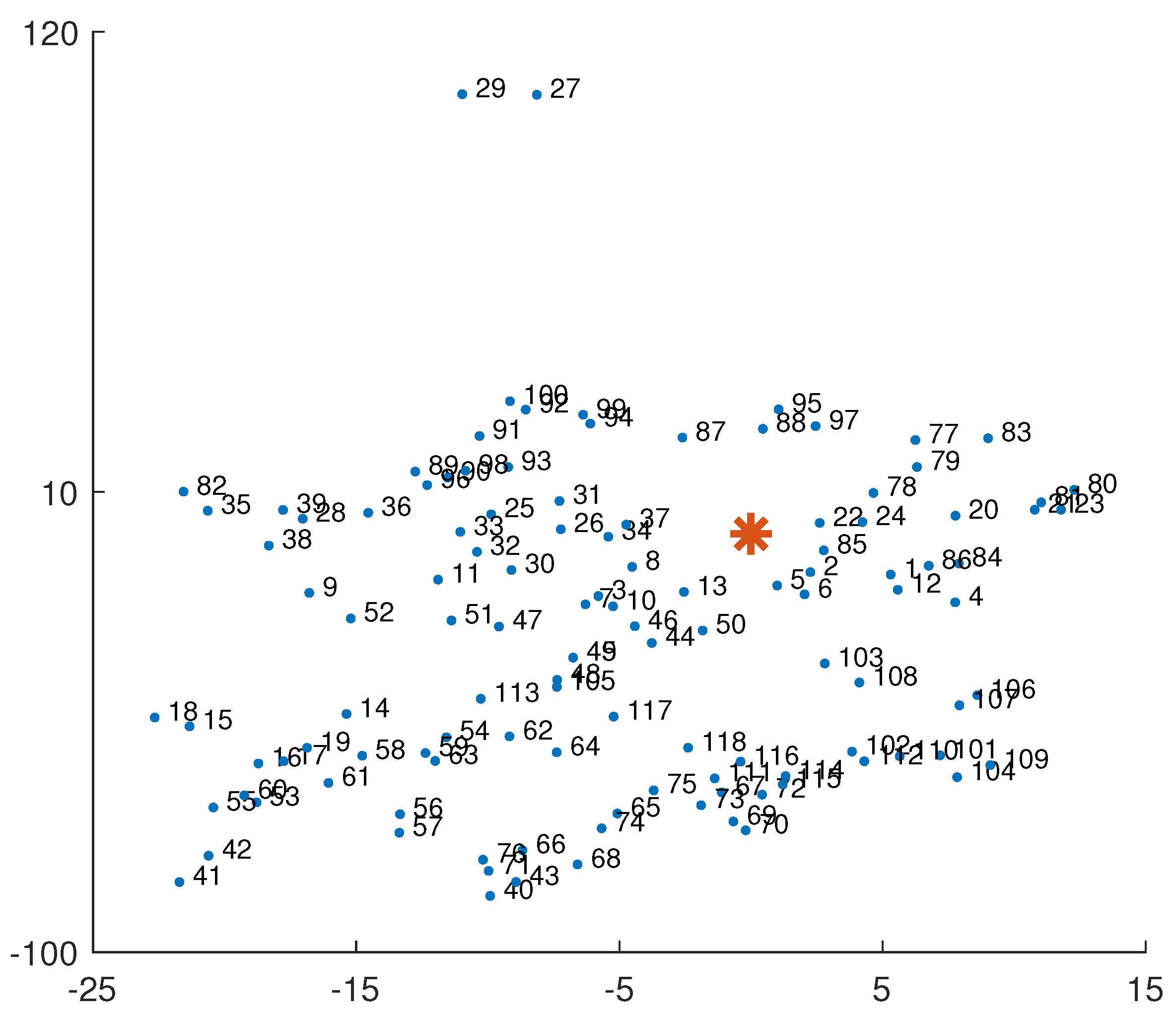
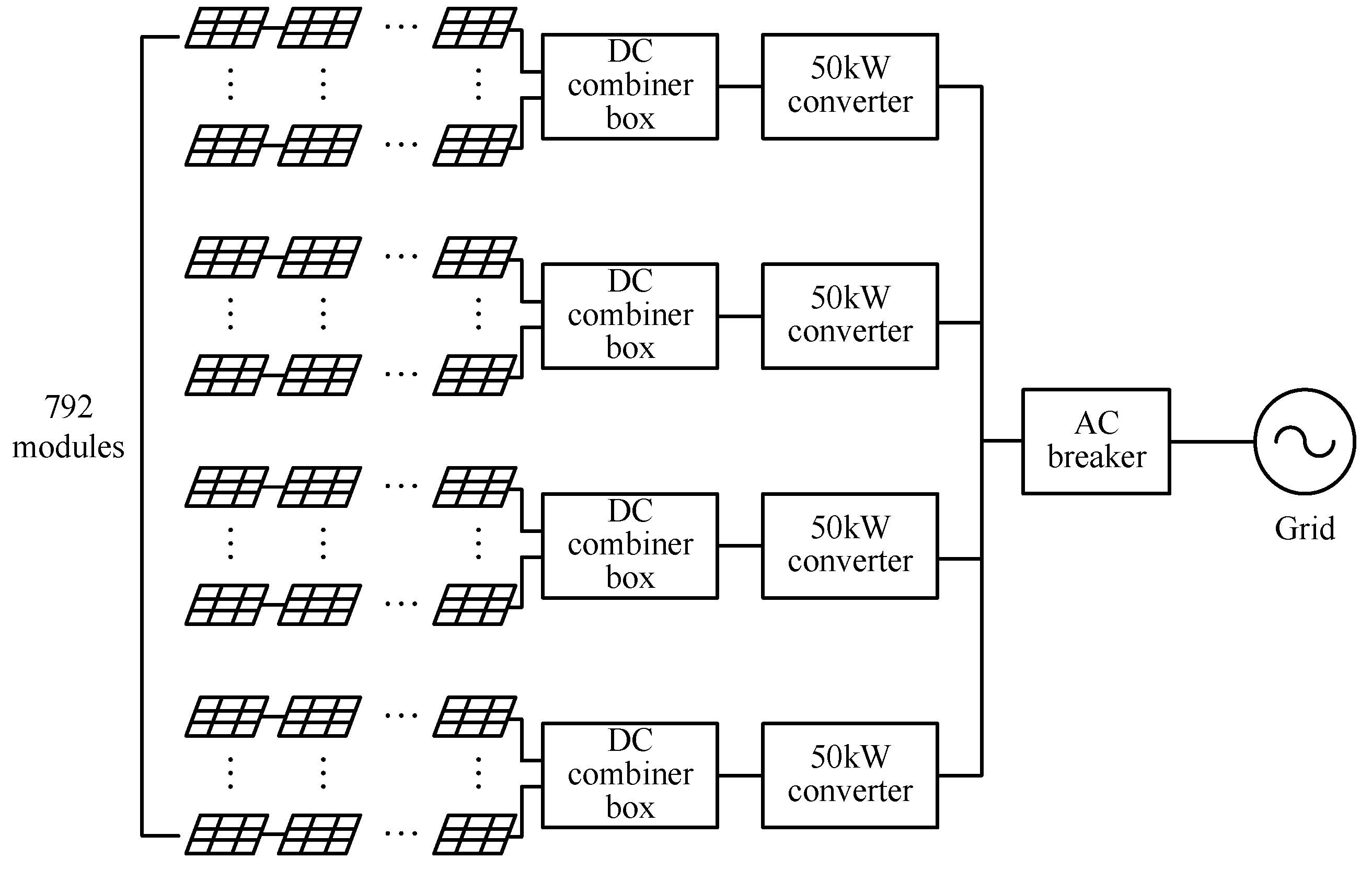
4.1. Structure of DPV Stations

This paper takes the DPV poverty alleviation project in Badong County, Hubei Province, as the research object. The project encompasses 118 village-level poverty alleviation DPV stations. All maintenance of all DPV stations in this project is outsourced to a third party, Badong Chaohui Company. The company has set up a maintenance center in Badong County to take charge of all 118 stations. The geographical distribution of the stations and the maintenance center are shown in Figure 4, where the red star and blue dots represent the maintenance center and the DPV stations, respectively. The maintenance center is the origin of the coordinates, with the x- and y-axes are distances in km.

As all stations have the same structure, this paper focuses on the modeling of their key components: 792 modules of 265 W, 4 DC combiner boxes, 4 string inverters of 50 kW, and 1 AC breaker. The structure is shown in Figure 5.

4.2. Failure Rate and Dust Accumulation Rate

According to the data provided in References [30,31], the failure rates of the DPV components are shown in

Table 1. The failure rates of the DPV components.

Component	Failures/h
PV module	0.33 × ${10}^{-6}$
DC combiner box	45.13 × ${10}^{-6}$
String inverter	12.90 × ${10}^{-6}$
AC circuit breaker	5.71 × ${10}^{-6}$

.

The number of modules connected to each type of DPV component is shown in

Table 2. The number of modules connected to each type of DPV component.

Component	Number of Modules
PV module	11
DC combiner box	198
String inverter	198
AC circuit breaker	792

.

In this paper, the empirical constant of the dust accumulation model is calculated according to the natural dust deposition data provided by Chaohui Company.

These data record the loss rate of power generation in Badong. The loss rates of the DPV stations on the 5th, 10th, 15th, 20th, 25th, and 30th days are 5.11%, 7.98%, 9.73%, 13.16%, 14.71%, and 16.45%, respectively. The empirical constants a = 22.71 and b = $-0.0439$ are obtained by fitting, so the power generation loss rate caused by dust is

$$\begin{array}{c}\hfill \begin{array}{c}\hfill {\eta }_{\mathrm{ash}}\left(d\right)=22.71·(1-exp(-0.0439·d))\times 100\%\end{array}\end{array}$$

(26)

The output power $P\left(t\right)$ of the DPV stations at time t is calculated based on the annual average hourly output curve of typical DPV in Badong, as shown in Figure 6.

4.3. Economic Parameters

In this paper, CNY is used as the unit, where 1 USD = 7.16437 CNY. According to the maintenance data of Chaohui Company, the grid-connected electricity price $p_{\mathrm{el}}$ is 0.4 CNY/(kWh); the fuel cost $c_{\mathrm{vel}}$ is 2 CNY/km, and the driving speed v is 60 km/h; the cleaning cost of one station $c_{\mathrm{cl}}$ is CNY 200, and the time spent cleaning the dust of one station $t_{\mathrm{cl}}$ is 4 h. The time spent fixing each failed component $t_{\mathrm{fix}}$ is 2 h. The daily base salary $c_{\mathrm{bs}}$ is CNY 300, the hourly wage $c_{\mathrm{w}}$ is CNY 50, and the maximum working time $wl$ is 10 h.

5. Results and Discussion

The hardware environment used for the simulation in this paper is the i9 13900k processor, and the software application is Matlab. The simulation can be completed in about 20 min by using this equipment.

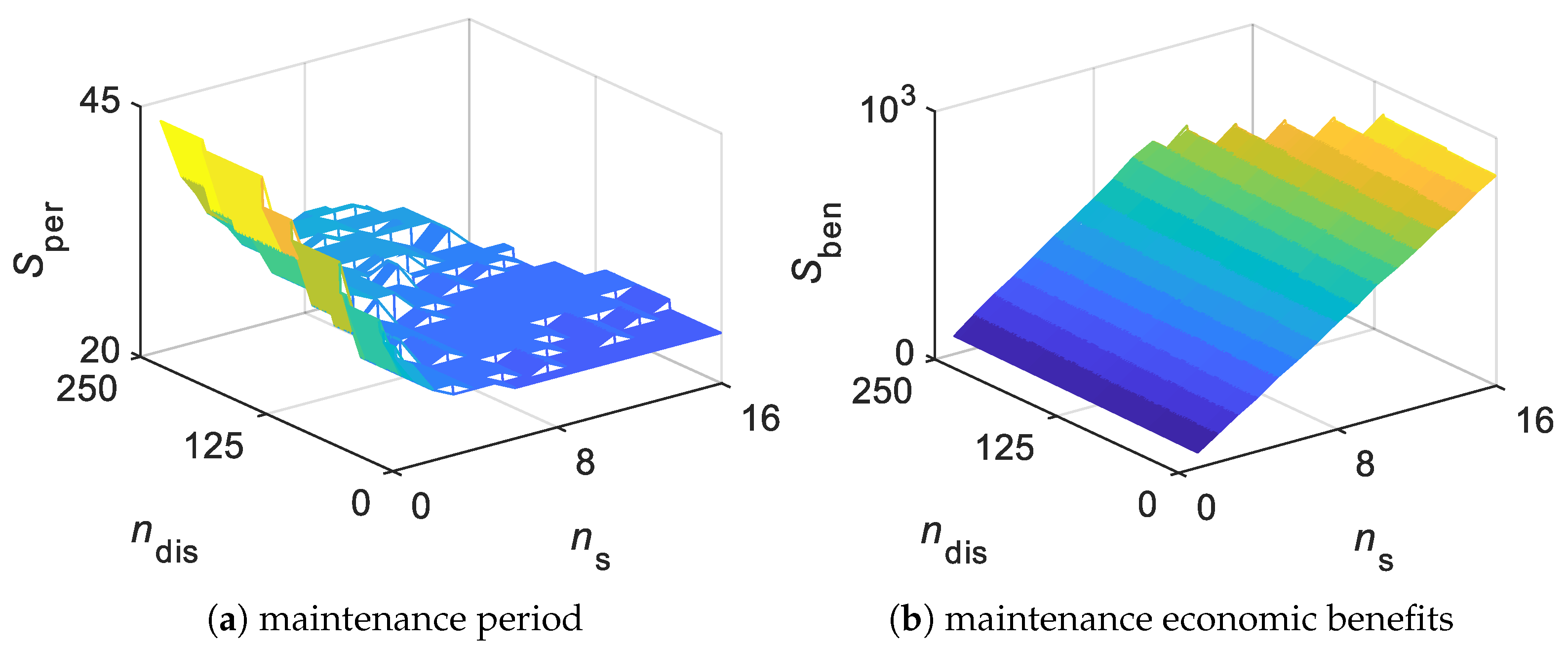
5.1. Results of Maintenance Period Decision Model

In order to compare the optimal maintenance period of different numbers of DPV stations and different driving distance in one area, three typical scenarios are set up in this paper.

Scenario I: one station; 1 km driving distance.

Scenario II: one station; 200 km driving distance.

Scenario III: 10 stations; 1 km driving distance.

The average results of 10,000 simulations for the three scenarios are shown in Figure 7. In Figure 7, the horizontal coordinate of the lowest point of the blue line is the optimal maintenance period, and its vertical coordinate is $C_{\mathrm{mean}}$. For the optimal average daily maintenance economic benefits, in Scenario I, the optimal maintenance period is 30 days, $C_{\mathrm{mean}}$ = CNY 59.2, $C_{\mathrm{fai}}$ = CNY 6.8, $C_{\mathrm{dust}}$ = CNY 27.7, $C_{\mathrm{vel}}$ = CNY 0.0667, $C_{\mathrm{cl}}$ = CNY 6.7, $C_{\mathrm{bs}}$ = CNY 10.1, and $C_{\mathrm{w}}$ = CNY 7.9.

In Scenario II, the optimal maintenance period is 43 days, $C_{\mathrm{mean}}$ = CNY 70.0, $C_{\mathrm{fai}}$ = CNY 9.4, $C_{\mathrm{dust}}$ = CNY 33.7, $C_{\mathrm{vel}}$ = CNY 9.3, $C_{\mathrm{cl}}$ = CNY 4.7, $C_{\mathrm{bs}}$ = CNY 7.1, and $C_{\mathrm{w}}$ = CNY 5.9.

In Scenario III, the optimal maintenance period is 25 days, $C_{\mathrm{mean}}$ = CNY 538.7, $C_{\mathrm{fai}}$ = CNY 56.5, $C_{\mathrm{dust}}$ = CNY 247.6, $C_{\mathrm{vel}}$ = CNY 0.08, $C_{\mathrm{cl}}$ = CNY 80.0, $C_{\mathrm{bs}}$ = CNY 62.4, and $C_{\mathrm{w}}$ = CNY 92.2.

Figure 7 illustrates that as the maintenance period lengthens, several factors undergo changes. Specifically, the number of failed components increases, failure time increases, and dust accumulation worsens. Consequently, power generation loss costs increase across all three scenarios. However, there is a trade-off: the number of annual maintenance events decreases, along with the total maintenance time. As a result, overall maintenance costs decrease for all three scenarios.

The power generation loss costs in the three scenarios are all mainly caused by module dust, which is consistent with the actual situation of low failure rates for DPV. In addition, the power generation loss cost almost increases in proportion to the increment of the number of stations, because of the similarity of the DPV stations in this paper.

Regarding maintenance costs, in Scenario I, they mainly refer to the base salary, and in Scenario III, they mainly refer to the hourly wage. As can be seen from the figure, the daily workload of maintainers is unsaturated if just one station is maintained as an area, leading to higher labor costs. As the number of stations in the area increases, the workload of each maintainer also increases, and the proportion of basic salary in the maintenance cost gradually decreases. Additionally, the maintenance cost in Scenario II is mainly vehicle fuel cost, which increases consistently with the driving distance. For instance, an area with a 1 km driving distance incurs almost negligible fuel costs.

To further compare and analyze the impact of the number of stations and driving distance on the maintenance period, this paper draws a three-dimensional diagram of the maintenance period and maintenance economic benefits under different numbers of stations ($n_{\mathrm{s}}$ = 1, 2, …, 16) and different driving distances ($n_{\mathrm{d}}$ = 1, 2, …, 250), as shown in Figure 8. In the overall trend, the maintenance period tends to increase as the number of stations decreases or the driving distance increases, while the influence of the number of stations on the economic benefits outweighs that of the driving distance.

In the overall trend, the maintenance period tends to extend as the number of stations decreases or the driving distance increases. While the impact of the number of stations on the economic benefits outweighs that of driving distance.

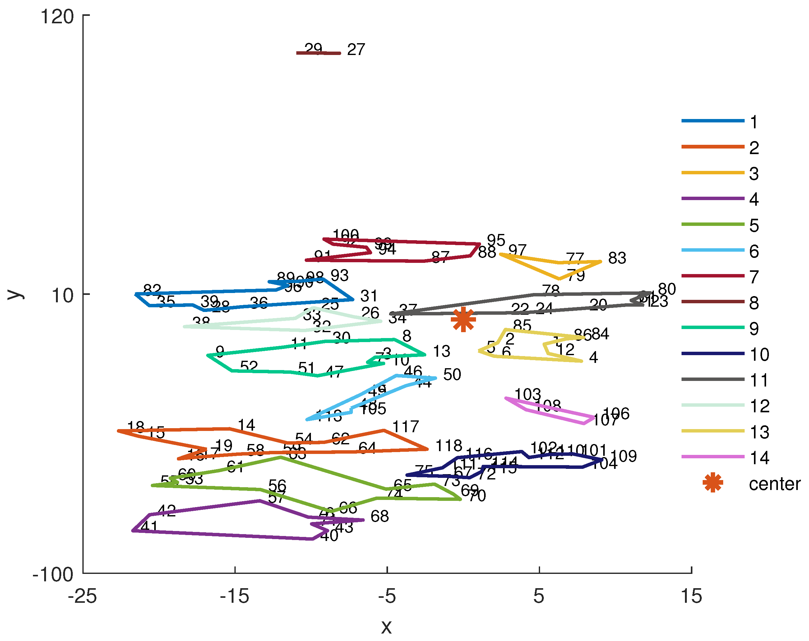
5.2. Results of Areal Maintenance Strategy

According to Equation (21), the maximum number of stations in the area is 19, so the range of $n_{\mathrm{s}}$ is [1, 19]. According to Equation (22), the maximum driving distance in the area is 300 km, so the value range of $n_{\mathrm{d}}$ is [1, 300]. The number of combinations of $n_{\mathrm{s}}$ and $n_{\mathrm{d}}$ is 5700 in total, and the combinations that do not satisfy the constraint on the driving distance are excluded through Equation (23). This paper substitutes all legal combinations into the maintenance period decision model to calculate $S_{\mathrm{per}}(n_{\mathrm{s}},n_{\mathrm{d}})$ and $S_{\mathrm{ben}}(n_{\mathrm{s}},n_{\mathrm{d}})$.

The IGA proposed in this paper is used to solve this problem. $N_{\mathrm{base}}=50$, $N_{\mathrm{top}}=50$, $M=1000$, $loop=1000$, and ${\mathrm{P}}_{\mathrm{m}}=0.1$. The fixed stations obtained from 50 suboptimal solutions are shown in

Table 3. The fixed stations.

Maintenance Area	Stations
1	89 90 93 96 98
2	16 17 58 59
3	77 83 79
4	40 41 42 43 68 71 76
5	65 66 69 70 73 74
6	44 105 113
7	87 91 92 94 99 100
8	27 29
9	51 52
10	67 72 101 102 104 109 110 112 114 115
11	20 21 23 80 81

. Take maintenance area 1 as an example; it represents stations 89, 90, 93, 96, and 98, which are fixed in the area. Stations 89, 90, 93, 96, and 98 are treated as fixed stations, and they are not solved by the top level of the IGA.

The optimal result of 50 suboptimal solutions is 6530.4. A total of 53 fixed stations are obtained, i.e., $N_{\mathrm{s},\mathrm{f}}=53$. The remaining 65 stations are unresolved stations, i.e., $N_{\mathrm{s},\mathrm{u}}=65$. Then, we recode and solve the unresolved stations, and the final results are shown in

Table 4. The specific results of the areal maintenance strategy.

Maintenance Area	Number of Stations	Driving Distance	${\mathit{S}}_{\mathbf{per}}$	${\mathit{S}}_{\mathbf{ben}}$	Number of Maintainers
1	11 (89 90 93 96 98 28 31, 35 36 39 82)	64	25	592.2	5
2	13 (16 17 58 59 14 15 18 19 54 62 64 117 118)	141	26	716.9	7
3	4 (77 83 79 97)	58	26	219.4	2
4	8 (40 41 42 43 68 71 76 57)	192	29	455.3	5
5	12 (65 66 69 70 73 74 53 55 56 60 61 63)	175	27	671.6	7
6	8 (44 105 113 45 46 48 49 50)	83	26	436.0	4
7	8 (87 91 92 94 99 100 88 95)	79	26	435.6	4
8	2 (27 29)	214	35	131.6	2
9	11 (51 52 3 7 8 9 10 11 13 30 47)	63	25	592.1	5
10	13 (67 72 101 102 104 109 110 112 114 115 75 111 116)	142	26	717.1	7
11	9 (20 21 23 80 81 22 24 37 78)	44	26	483.4	4
12	6 (25 26 32 33 34 38)	44	26	325.6	3
13	9 (1 2 4 5 6 12 84 85 86)	43	26	483.3	4
14	4 (103 106 107 108)	85	27	224.2	2

Note: The digital numbers in ( ) are the stations in the area.

. On the premise of obtaining the best economic benefits, the areal maintenance strategy of 118 stations divided into 11 regions is obtained, as shown in Figure 9. In Figure 9, each closed line represents a maintenance area, and there are 14 maintenance areas.

Maintenance area 1 is taken as an example to explain the result. This area includes 11 stations, including stations 89, 90, 93, 96, 98, 28, 31, 35, 36, 39, and 82. Among these stations, stations 89, 90, 93, 96, and 98 are fixed, which are solved at the base level of the IGA, while stations 28, 31, 35, 36, 39, and 82 are unresolved, which are solved at the top level of the IGA. The shortest driving distance from the maintenance center to traverse all the 11 stations and finally return is 64 km. The optimal economic benefit F can be achieved by maintaining these 11 stations in this area every 25 days. The sum of the average daily maintenance economic benefits in this area amounts to CNY 592.2.

Then, the sum of the average daily maintenance economic benefits of the 118 DPV stations is calculated to be $F=6484.2$. Based on the analysis, when compared with the traditional GA, the IGA method proposed in this paper can effectively improve search accuracy and prevent the model from falling into the local optimal solution. It is worth mentioning that 13 of the 50 top-level GAs have obtained the optimal solution, which further demonstrates the effectiveness of the proposed IGA method.

Currently, Chaohui Company continues to employ the traditional independent maintenance strategy, in which each station is regarded as a single area. The company assigns one maintainer to maintain one station every 30 days, and the daily maintenance economic benefits of the 118 stations is CNY 7272.1.

Compared with the traditional maintenance strategy, the strategy proposed in this paper can save CNY 787.9 per day and nearly CNY 300,000 per year, reducing the maintenance cost by 10.38%. Thus, the areal maintenance strategy proposed in this paper can effectively classify the stations, significantly reducing the maintenance economic costs of large-scale DPV.

To further verify the effectiveness of the method, the method proposed in Reference [22] is used to solve the research case of this paper. The method proposed in [22] is not exactly the same as that of this paper. The common point of the two methods is that both divide the maintenance areas. Unlike the method proposed in this paper, Reference [22] optimizes the location of the maintenance center but does not optimize the maintenance period of each area, and the maintenance period of each area is fixed to 1 month. Since the maintenance center has already been built in this research case, when using the method in [22], the location of the maintenance center is not optimized, and only the maintenance areas are divided. Solved by the method in Reference [22], the daily maintenance economic benefits amount to CNY 6647.1. Consequently, the results of this paper show an advantage (CNY 6484.2).

6. Conclusions

In this paper, an areal maintenance strategy is proposed to solve the problem of lack of efficient maintenance strategies for large-scale DPV.

Based on considering the reliability of the components and the dust deposition of the modules, a flexible DPV maintenance period decision model is established for one area, which can realize the determination of the optimal maintenance period under different parameters and quantitatively evaluate the maintenance economic benefits. The results indicate that the number of stations in the area significantly affects the economic benefits compared with the driving distance.

Based on the maintenance period decision model, an areal maintenance strategy is proposed to achieve the overall optimal maintenance benefits through the optimal division of all the stations. At the same time, the IGA method is proposed to solve the station classification problem.

The results indicate that the proposed strategy effectively classifies all the stations into different areas and generates reasonable maintenance plans for all the areas. Compared with the traditional maintenance strategy, the proposed strategy can save 10.38% of the maintenance cost, up to CNY 300,000 annually. Compared with the traditional GA, the proposed IGA method can effectively obtain the global optimal solution, and the solution is reliable.

The limitation of this paper is that it only demonstrates the optimal regional maintenance strategy in Badong County, Hubei Province, which may not be fully representative of all regions, so its generalizability will be demonstrated in future studies.

A further research directions is to refine the PV dust accumulation model according to different regions, environments, and seasons to enhance the accuracy of the method proposed in this paper.

References

1. Baek, Y.J.; Jung, T.Y.; Kang, S.J. Low carbon scenarios and policies for the power sector in Botswana. Clim. Policy 2019, 19, 219–230. [Google Scholar] [CrossRef]
2. Ji, Q.; Zhang, D. How much does financial development contribute to renewable energy growth and upgrading of energy structure in China? Energy Policy 2019, 128, 114–124. [Google Scholar] [CrossRef]
3. National Energy Administration. Construction and Operation of Photovoltaic Power Generation in 2023. Available online: https://www.nea.gov.cn/2024-02/28/c_1310765696.htm (accessed on 28 February 2024).
4. Zhang, A.H.; Sirin, S.M.; Fan, C.; Bu, M. An analysis of the factors driving utility-scale solar PV investments in China: How effective was the feed-in tariff policy? Energy Policy 2022, 2022, 113044. [Google Scholar] [CrossRef]
5. Li, Y.; Zhang, Q.; Wang, G.; McLellan, B.; Liu, X.F.; Wang, L. A review of photovoltaic poverty alleviation projects in China: Current status, challenge and policy recommendations. Renew. Sustain. Energy Rev. 2018, 94, 214–223. [Google Scholar] [CrossRef]
6. Rahman, M.M.; Khan, I.; Alameh, K. Potential measurement techniques for photovoltaic module failure diagnosis: A review. Renew. Sustain. Energy Rev. 2021, 151, 111532. [Google Scholar] [CrossRef]
7. Osmani, K.; Haddad, A.; Lemenand, T.; Castanier, B.; Ramadan, M. A review on maintenance strategies for PV systems. Sci. Total Environ. 2020, 746, 141753. [Google Scholar] [CrossRef]
8. Iftikhar, H.; Sarquis, E.; Branco, P.C. Why can simple operation and maintenance (O&M) practices in large-scale grid-connected PV power plants play a key role in improving its energy output? J. Abbr. 2021, 14, 3798. [Google Scholar]
9. Yuan, J.; Sun, S.; Zhang, W.; Xiong, M. The economy of distributed PV in China. Energy 2014, 78, 939–949. [Google Scholar] [CrossRef]
10. Perdue, M.; Gottschalg, R. Energy yields of small grid connected photovoltaic system: Effects of component reliability and maintenance. IET Renew. Power Gener. 2015, 9, 432–437. [Google Scholar] [CrossRef]
11. Siemer, J. Operation & Maintenance. 2016, pp. 36–39. Available online: https://kh.aquaenergyexpo.com/wp-content/uploads/2023/01/Operation-Maintenance-Best-Practice-Guidelines.pdf (accessed on 19 August 2024).
12. Enbar, N.; Weng, D.; Klise, G.T. Budgeting for Solar PV Plant Operations & Maintenance: Practices and Pricing; Sandia National Lab. (SNL-NM): Albuquerque, NM, USA, 2016.
13. Zhang, P.; Li, W.; Li, S.; Wang, Y.; Xiao, W. Reliability assessment of photovoltaic power systems: Review of current status and future perspectives. Appl. Energy 2013, 104, 822–833. [Google Scholar] [CrossRef]
14. Collins, E.; Dvorack, M.; Mahn, J.; Mundt, M.; Quintana, M. Reliability and availability analysis of a fielded photovoltaic system. In Proceedings of the 2009 34th IEEE Photovoltaic Specialists Conference (PVSC), Philadelphia, PA, USA, 7–12 June 2009; pp. 002316–002321. [Google Scholar]
15. Ahadi, A.; Ghadimi, N.; Mirabbasi, D. Reliability assessment for components of large scale photovoltaic systems. J. Power Sources 2014, 264, 211–219. [Google Scholar] [CrossRef]
16. Sanjari, M.J.; Gooi, H. Probabilistic forecast of PV power generation based on higher order Markov chain. IEEE Trans. Power Syst. 2016, 32, 2942–2952. [Google Scholar] [CrossRef]
17. Lu, H.; Zhao, W. Effects of particle sizes and tilt angles on dust deposition characteristics of a ground-mounted solar photovoltaic system. Appl. Energy 2018, 220, 514–526. [Google Scholar] [CrossRef]
18. Darwish, Z.A.; Kazem, H.A.; Sopian, K.; Al-Goul, M.; Alawadhi, H. Effect of dust pollutant type on photovoltaic performance. Renew. Sustain. Energy Rev. 2015, 41, 735–744. [Google Scholar] [CrossRef]
19. Zaihidee, F.M.; Mekhilef, S.; Seyedmahmoudian, M.; Horan, B. Dust as an unalterable deteriorative factor affecting PV panel’s efficiency: Why and how. Renew. Sustain. Energy Rev. 2016, 65, 1267–1278. [Google Scholar] [CrossRef]
20. Muñoz-Cerón, E.; Lomas, J.; Aguilera, J.; de la Casa, J. Influence of Operation and Maintenance expenditures in the feasibility of photovoltaic projects: The case of a tracking pv plant in Spain. Energy Policy 2018, 121, 506–518. [Google Scholar] [CrossRef]
21. Zheng, Y.; Xia, Z.; Luo, Y.; Chen, Y.; Zhou, L.; Peng, J. Research on operation and maintenance mode of photovoltaic poverty alleviation power station based on fuzzy analytic hierarchy process. Electr. Power 2021, 54, 191–198. [Google Scholar]
22. Carrasco, L.; Martín-Campo, F.J.; Narvarte, L.; Ortuño, M.T.; Vitoriano, B. Design of maintenance structures for rural electrification with solar home systems. The case of the Moroccan program. Energy 2016, 117, 47–57. [Google Scholar] [CrossRef]
23. Villarini, M.; Cesarotti, V.; Alfonsi, L.; Introna, V. Optimization of photovoltaic maintenance plan by means of a FMEA approach based on real data. Energy Convers. Manag. 2017, 152, 1–12. [Google Scholar] [CrossRef]
24. Hammad, B.; Al-Abed, M.; Al-Ghandoor, A.; Al-Sardeah, A.; Al-Bashir, A. Modeling and analysis of dust and temperature effects on photovoltaic systems’ performance and optimal cleaning frequency: Jordan case study. Renew. Sustain. Energy Rev. 2018, 82, 2218–2234. [Google Scholar] [CrossRef]
25. ISO 9000:2015; Quality Management Systems—Fundamentals and Vocabulary. International Standards Organization: Geneva, Switzerland, 2015.
26. Jardine, A.K.; Tsang, A.H. Maintenance, Replacement, and Reliability: Theory and Applications; CRC Press: Boca Raton, FL, USA, 2005. [Google Scholar]
27. Spertino, F.; Chiodo, E.; Ciocia, A.; Malgaroli, G.; Ratclif, A. Maintenance activity, reliability, availability, and related energy losses in ten operating photovoltaic systems up to 1.8 MW. IEEE Trans. Ind. Appl. 2020, 57, 83–93. [Google Scholar] [CrossRef]
28. Jones, R.K.; Baras, A.; Al Saeeri, A.; Al Qahtani, A.; Al Amoudi, A.O.; Al Shaya, Y.; Alodan, M.; Al-Hsaien, S.A. Optimized cleaning cost and schedule based on observed soiling conditions for photovoltaic plants in central Saudi Arabia. IEEE J. Photovoltaics 2016, 6, 730–738. [Google Scholar] [CrossRef]
29. Zhao, Y.; Ball, R.; Mosesian, J.; de Palma, J.F.; Lehman, B. Graph-based semi-supervised learning for fault detection and classification in solar photovoltaic arrays. IEEE Trans. Power Electron. 2014, 30, 2848–2858. [Google Scholar] [CrossRef]
30. Gallardo-Saavedra, S.; Hernández-Callejo, L.; Duque-Pérez, O. Quantitative failure rates and modes analysis in photovoltaic plants. Energy 2019, 183, 825–836. [Google Scholar] [CrossRef]
31. Colli, A. Failure mode and effect analysis for photovoltaic systems. Renew. Sustain. Energy Rev. 2015, 50, 804–809. [Google Scholar] [CrossRef]
Figure 1. Bathtub curve.
Electronics 13 03593 g001
Figure 2. Pseudocode of DPV maintenance period decision model.
Electronics 13 03593 g002
Figure 3. An example for N base suboptimal solutions.
Electronics 13 03593 g003
Figure 4. The geographical distribution of the DPV stations and the maintenance center in Badong County.
Electronics 13 03593 g004
Figure 5. The structure of the DPV stations.
Electronics 13 03593 g005
Figure 6. The annual average hourly output power.
Electronics 13 03593 g006
Figure 7. The optimal maintenance period results for the three scenarios.Scenario I: 1 station, 1 km driving distance.Scenario II: 1 station, 200 km driving distance.Scenario III: 10 stations, 1 km driving distance.
Electronics 13 03593 g007
Figure 8. The maintenance period and economic benefits under different numbers of stations and different driving distances.
Electronics 13 03593 g008
Figure 9. The annual average hourly output power.
Electronics 13 03593 g009