Forecasting Flower Prices by Long Short-Term Memory Model with Optuna

Abstract

The oriental lily ‘Casa Blanca’ is one of the most popular and high-value flowers. The period for keeping these flowers refrigerated is limited. Therefore, forecasting the prices of oriental lilies is crucial for determining the optimal planting time and, consequently, the profits earned by flower growers. Traditionally, the prediction of oriental lily prices has primarily relied on the experience and domain knowledge of farmers, lacking systematic analysis. This study aims to predict daily oriental lily prices at wholesale markets in Taiwan using many-to-many Long Short-Term Memory (MMLSTM) models. The determination of hyperparameters in MMLSTM models significantly influences their forecasting performance. This study employs Optuna, a hyperparameter optimization technique specifically designed for machine learning models, to select the hyperparameters of MMLSTM models. Various modeling datasets and forecasting time windows are used to evaluate the performance of the designed many-to-many Long Short-Term Memory with Optuna (MMLSTMOPT) models in predicting daily oriental lily prices. Numerical results indicate that the developed MMLSTMOPT model achieves highly satisfactory forecasting accuracy with an average mean absolute percentage error value of 12.7%. Thus, the MMLSTMOPT model is a feasible and promising alternative for forecasting the daily oriental lily prices.

1. Introduction

In Taiwan, oriental lilies are highly popular and represent a significant portion of the fresh flowers traded in auction markets. Oriental lilies hold considerable value as agricultural products due to their ornamental and symbolic significance, making them suitable for a variety of occasions, including weddings, funerals, birthday parties, and festive celebrations. As high-value crops, flowers are among the most important agricultural products in Taiwan.

Currently, the production and marketing of flowers in Taiwan involve cultivating and harvesting crops, followed by distribution through five major flower auction markets located in Taipei, Taichung, Changhua, Tainan, and Kaohsiung. Farmers typically decide which wholesale market to transport their flowers based on recent trading prices. Alternatively, farmers may store flowers in cold storage and wait for better prices. However, marketing strategies are usually based on farmers’ experiences, and misjudgments can result in profit losses. Therefore, a reliable price forecasting method is essential to help farmers accurately capture flower auction prices and develop effective sales strategies to increase their profits.

Sun et al. [1] and Wang et al. [2] have conducted comprehensive reviews of price forecasting for various agricultural products, including soybean [3,4,5,6,7,8], cabbage or vegetable [9,10,11,12,13], potato [10,14], pork [10,15,16], egg [17,18], fish [10], garlic [19], corn [3,8,20], carrot [21], apple [22], orange [23], cassava [24], and cotton and coffee [3]. However, studies on forecasting flower prices, particularly for oriental lilies, are limited. Factors affecting flower prices encompass both supply and demand aspects, such as climate change, pests and diseases, seedling sources, planting area, holidays [25], policy factors [26], and population sizes [27]. Therefore, predicting prices for flowers and other agricultural products is inherently challenging.

Methods for predicting agricultural product prices can be categorized into three main types: traditional forecasting methods, intelligent forecasting methods, and hybrid forecasting methods [1,2]. Traditional methods are statistically based, such as the Autoregressive Integrated Moving Average (ARIMA) model. For instance, Kathayat and Dixit [28] used the ARIMA model to predict wholesale rice prices for the following year, demonstrating that the model was suitable for regions with distinct seasonal price variations. Agbo [29] utilized ARIMA models to forecast the price fluctuations of various crops, including green beans, tomatoes, onions, oranges, grapes, and strawberries. The study demonstrated that ARIMA models are generally effective for most of these crops. In contrast, Zhao [30] found that support vector machines (SVMs) outperformed ARIMA in univariate models for agricultural price forecasting. Recently, the long short-term memory (LSTM) model has gained popularity in this field. Yuan and Ling [31] showed that LSTM models provide superior accuracy compared to ARIMA, support vector regression, Prophet, and extreme gradient boosting when forecasting multi-factor data. In another study, Purohit et al. [32] developed a hybrid model that combined ARIMA, LSTM, and SVM to forecast vegetable prices in India, achieving better forecasting accuracy than any single model. Similarly, Guo et al. [20] designed a hybrid model integrating LSTM, ARIMA, and backpropagation neural networks to predict corn prices, with results indicating satisfactory forecasting performance. However, Nassar et al. [33] argued that a simple LSTM model could outperform more complex hybrid networks in certain scenarios. Harshith and Kumari [34] proposed a stacked LSTM model using daily data to predict cumin prices, finding it superior to other models for long-term predictions. Zhang and Tang [35] developed a hybrid model with quadratic decomposition technology to forecast agricultural products like wheat, corn, and sugar, achieving higher predictive accuracy than other models. Zhang et al. [36] utilized an LSTM model to predict the prices of six different types of vegetables in Beijing. Their findings demonstrated that the LSTM model outperformed other time-series machine learning models, including Convolutional Neural Network (CNN), Support Vector Regression (SVR), and eXtreme Gradient Boosting (XGBoost), in terms of prediction accuracy. Similarly, Kang et al. [37] developed an LSTM model for predicting banana prices, incorporating a chaotic particle swarm algorithm to optimize the hyperparameters. The experimental results indicated that the hyperparameter-optimized LSTM model achieved superior accuracy and stability in predicting banana prices. Rana et al. [38] employed the LSTM model to forecast spinach prices, reporting that it provided more accurate results than the ARIMA and random forest models. Furthermore, this study pointed out that properly selecting hyperparameters for LSTM models can improve forecasting performance. The investigation revealed that the LSTM model is a very promising method for forecasting prices of agricultural products [38,39,40].

The aim of this study is to employ MMLSTM (many-to-many Long Short-Term Memory) models using daily transaction prices of oriental lilies collected at the Taipei flower wholesale market. Various modeling datasets and forecasting time windows are performed to evaluate forecasting performance. Additionally, the Optuna framework [41] is utilized to optimize the hyperparameters of MMLSTM, namely, MMLSTMOPT, models for predicting daily oriental lily prices. The hyperparameters optimized for the MMLSTMOPT models include the optimizer, the number of neurons in MMLSTM layers, the number of neurons in the fully connected layer, the loss function, the number of epochs, the batch size, and the learning rate. A brief summary of results obtained by MMLSTMOPT, MMLSTM, ARIMA, and Prophet [42] is illustrated in

Table 1. A brief summary of results.

Models	MSE	MAE	RMSE	MAPE	R2
MMLSTMOPT_21 days_AVG	634.22	17.89	24.68	12.70%	0.63
MMLSTM_21 days_AVG	700.07	18.56	25.94	13.21%	0.59
ARIMA (3, 1, 1)	1742.61	34.24	41.74	26.97%	−0.02
Prophet	2618.27	42.41	51.17	35.99%	−0.54

.

The structure of this study is as follows: Section 2 describes the long short-term memory method and the Optuna framework. Section 3 presents the proposed MMLSTMOPT models for predicting oriental lily prices. Section 4 discusses the numerical results and findings. Finally, conclusions are presented in Section 5.

2. Long Short-Term Memory and the Optuna Framework

2.1. Long Short-Term Memory

The long short-term memory model [43] is a variant of recurrent neural networks commonly used for handling sequential data. Compared to recurrent neural networks, LSTM models can capture long-term dependencies [44], and are suitable for processing time-series data. The LSTM model consists of one or more LSTM units, as illustrated in Figure 1. Each unit contains three key gates, namely, the forget gate, the input gate, and the output gate [45,46]. Gates help control the flow of information and effectively capture long-term dependencies within the sequence. In an LSTM unit, the forget gate and the input gate receive the current and previous hidden states then turn out to be the unit’s current state. Subsequently, the unit’s state is propagated sequentially and transmits information with minimal decay. Therefore, the unit can retain information over extended time periods. The mathematical representation of LSTM models is given by Equations (1)–(6).

$$f_t=\sigma \left(w_{f_x{x}_t}+w_{f_h{h}_{t-1}}+b_f\right)$$

(1)

$$i_t=\sigma \left(w_{i_x{x}_t}+w_{i_h{h}_{t-1}}+b_i\right)$$

(2)

$$g_t=\mathrm{t}\mathrm{a}\mathrm{n}\mathrm{h}(w_{g_x{x}_t}+w_{g_h{h}_{t-1}}+b_g)$$

(3)

$$o_t=\sigma (w_{o_x{x}_t}+w_{o_h{h}_{t-1}}+b_o)$$

(4)

$$C_t=g_t{i}_t+C_{t-1}{f}_t$$

(5)

$$h_t=\mathrm{t}\mathrm{a}\mathrm{n}\mathrm{h}\left(C_t\right)o_t$$

(6)

where $W$ is the weight, $b$ denoted the bias, $\sigma$ represents the sigmoid function, $C_{t-1}$ is the cell state at time $t-1$, $h_{t-1}$ is the hidden state at time $t-1$, $x_t$ expresses the input of the LSTM unit at the moment, $f_t$ is the output of the forget gate, $i_t$ is the output of the input gate, $o_t$ is the output of the output gate, $C_t$ is the current cell state, and $h_t$ is the current hidden state.

2.2. The Optuna Framework

The Optuna framework is a Python package designed for hyperparameter optimization [41], offering a simple and flexible interface for tuning machine learning models. The stages of the Optuna framework are depicted as follows. First, determine the hyperparameters, types of hyperparameters (such as integers, floats, and categorical values), and the searching boundaries for Optuna. Next, define an objective function that receives a trial as input and returns a value to be minimized or maximized. Optuna attempts to determine hyperparameters that optimize the objective function. The framework also allows users to query and record the values of hyperparameters during the optimization process. Finally, specify the number of Optuna trials to run. Additionally, some techniques, such as the timeout setting, sampling approaches, and pruning methods, can be used for adjusting the hyperparameters searching process. The sampling approaches include the random sampler, Tree-structured Parzen Estimator (TPE), Covariance Matrix Adaptation Evolution Strategy (CMA-ES), and grid sampler [41,47,48]. The pruning methods, which can terminate unsatisfactory trials early to save computational resources and time, include the base pruner, median pruner, successive halving pruner, hyperband pruner, threshold pruner, percentile pruner, and patient pruner [48,49].

3. The Proposed MMLSTMOPT Model for Forecasting Daily Oriental Lily Prices

In this study, the many-to-many long short-term memory (MMLSTM) model is employed to forecast the daily prices of oriental lilies. The Optuna framework is utilized to select the hyperparameters for the MMLSTM models. Figure 2 illustrates the developed MMLSTMOPT model for predicting daily prices of oriental lilies. The developed MMLSTMOPT model contains three parts, namely, data collection and preprocessing, determining, and training model, and performance evaluation. Historical price data from the past 7, 14, 21, and 28 days are used to predict prices for the following 1 to 7 days, resulting in a total of 28 different MMLSTMOPT models. In other words, four training datasets are employed to forecast seven time periods, respectively. The MMLSTMOPT model is performed by using Optuna to determine hyperparameters. Finally, the performance of MMLSTMOPT models is evaluated in forecasting daily prices of oriental lilies.

3.1. Data Collection and Preprocessing

The data collection period spanned from 1 January 2016, to 31 December 2020, during which a total of 1827 records of oriental lily auction average prices were gathered. The data were sourced from the “Agricultural Products Wholesale Market Transaction Information Network” (https://amis.afa.gov.tw accessed on 11 August 2023). A web scraping program was used to automatically extract daily auction daily average price data for various subcategories of oriental lilies. The data were gathered using a web scraping program built with the Selenium toolkit (https://www.selenium.dev/ accessed on 11 August 2023). The process involved first identifying the structure and locations of the target data on the webpage. The Selenium toolkit then simulated browser operations to automatically navigate to the relevant webpages and extract the necessary data. Due to the dynamic and complex nature of agricultural product transaction information, the automated program included error-handling mechanisms to address issues such as webpage loading delays or changes in data formats. The extracted data were then organized, and the daily prices of oriental lilies were compiled into structured datasets for the subsequent stage.

According to Chen et al. [50], data preprocessing, including handling missing values and data normalization, plays a crucial role in improving the accuracy and efficiency of forecasting models. The daily price data for oriental lilies contain missing values due to holidays when auctions do not occur, resulting in gaps in the transaction records. These missing values affect the accuracy of forecasting models [51,52]. One popular technique for addressing missing values of time-series data is the K-nearest neighbor (KNN) algorithm [53,54,55]. The KNN algorithm classifies data based on the Euclidean distance between data, and the average of K nearest samples serves as the missing value. In this study, the KNN approach was employed to address missing values. Missing values are calculated by the weighted imputation represented as Equation (7) [56].

$$y_{{miss}_t}^{*}={\displaystyle \frac{\sum _{j=1}^k{w}_j{u}_j}{\sum _{j=1}^k{w}_j}}$$

(7)

where $y_{{miss}_t}^{*}$ represents the estimated missing value at time t by a weighted mean, $k$ indicates the number of closest observations employed, $j$ is the observation of $k$, $\mathrm{a}\mathrm{n}\mathrm{d}{w}_j$ is the weight of the $k$-th closest neighbor observation with Equation (8).

$$w_j={\displaystyle \frac{1}{{d(y_{aj},y_{bj})}^2}}$$

(8)

where $d\left(y_{aj},y_{bj}\right)$ represents the distance between the missing data point and the $j$-th neighbor, and $u_j$ specifies the value corresponding to the $j$th nearest neighbor. Another essential data preprocessing procedure used in this investigation is normalization, which standardizes data to mitigate the influence of varying data distributions. Min–max normalization [57,58,59] was employed in this study to ensure that data from different ranges were standardized appropriately. The KNN algorithm and normalization were used in the data preprocessing stage. Then, the preprocessed data were input into MMLSTM models and MMLSTMOPT models. The values of preprocessed data were fixed after the KNN algorithm and normalization were conducted.

The data were separated into three parts, namely, the training dataset, the validation dataset, and the testing dataset. The training data were used to determine MMLSTM hyperparameters and to train the MMLSTM models. The wholesale price data from 2016 to 2018 were designated as the training dataset. The validation dataset was used to avoid overfitting during the training process, with the wholesale price data from 2019 serving this purpose. The model with the smallest loss on the validation data was selected for forecasting. To evaluate the forecasting performance, the wholesale price data in 2020 were designated as the testing dataset. The testing datasets are used to evaluate the finalized MMLSTMOPT models.

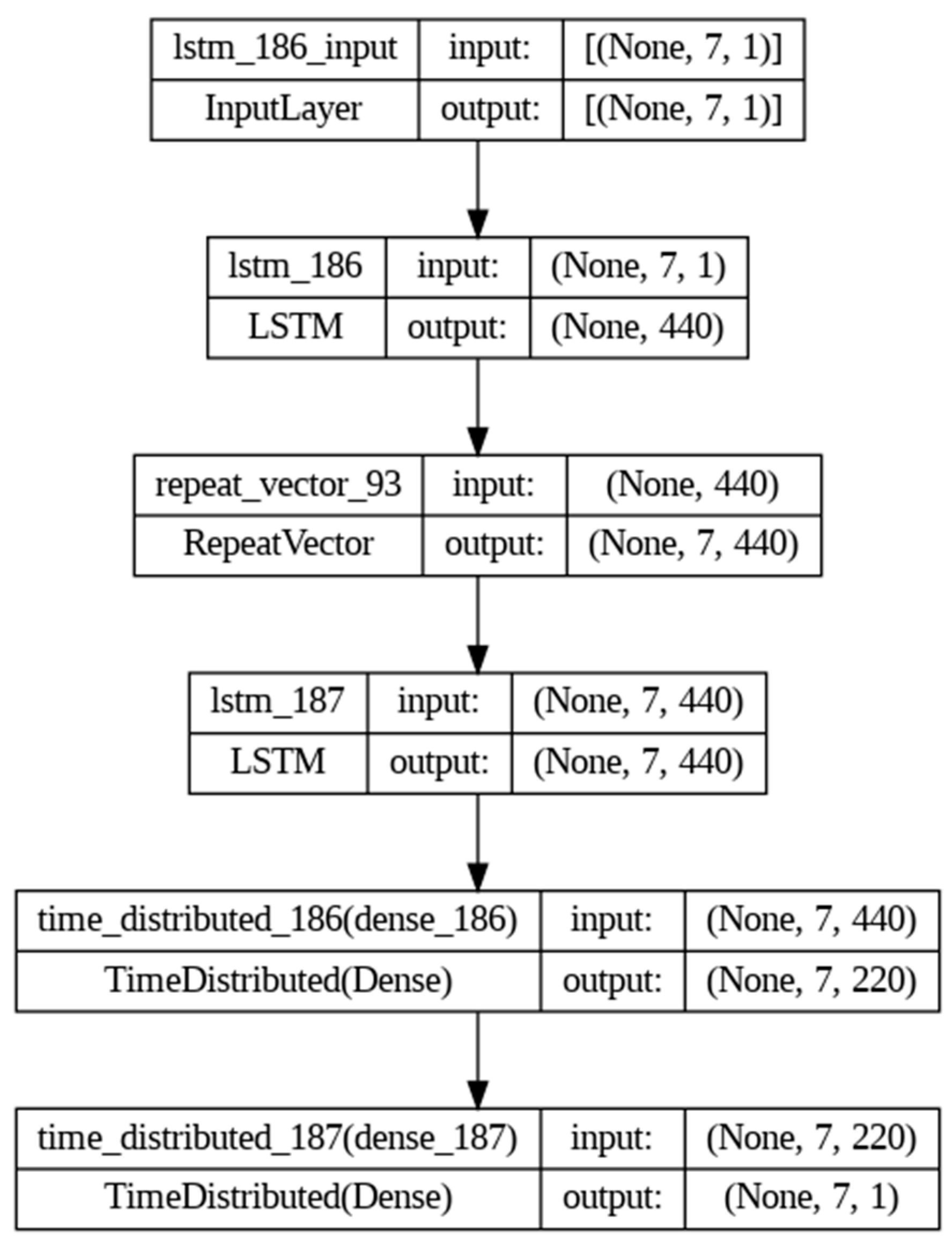
3.2. The Many-to-Many LSTM Model

LSTM models perform various time-series prediction tasks, including one-to-one, one-to-many, many-to-many, and many-to-one modes. Rao and Reimher [60] employed neural networks to develop a non-linear function-on-function regression model. The study pointed out that the proposed model is able to cope with many-to-many time-series data. Forecasting the next value based on the current data point, the one-to-one LSTM is the simplest model and is applicable to single-step prediction in time series [61]. The one-to-many LSTM model generates a series of future values from a single time point [62]. The many-to-many LSTM model includes two different types: the equal-length sequences model and the different-length sequences model. For the equal-length sequences model, the input and output sequences are of the same length, commonly used for synchronous transformations in time series. The different length sequences model is typically used in tasks like machine translation, where a sentence in one language is translated into another language with a potentially different number of words [63]. The many-to-one LSTM model has multiple inputs corresponding to a single output and is useful in tasks where predictions are based on a series of historical data points [64].

In this study, the many-to-many LSTM (MMLSTM) models were employed to forecast daily oriental lily prices. Figure 3 illustrates 28 MMLSTM models with various input and output data lengths used for predicting the daily prices of oriental lilies. The many-to-many model features an encoder–decoder structure, which consists of an encoder, an intermediate vector, and a decoder. Both the encoder and the decoder consist of one or more layers of LSTM structures [65]. The specific MMLSTM model used in this study has six layers. Figure 4 presents the six-layer MMLSTM model to forecast daily oriental lily prices. The MMLSTM model uses 7 days of daily oriental lily prices for modeling and forecasting the prices for the following 7 days. The Optuna was employed to determine the hyperparameters of the second layer, the fourth layer, and the fifth layer. The first layer is an input layer. The second layer acts as the initial layer of the sequence-to-sequence model and functions as the encoder in the prediction model. In this study, the model receives input data of historical prices with ranges of 7 days, 14 days, 21 days, and 28 days, resulting in four different modeling datasets. This layer processes these historical price sequences and only returns the output of the last time step. This setup allows the model to integrate the entire historical data sequence to predict the next time point. The third layer expands the single output from the previous LSTM layer into a repeated sequence of the same length as the target output sequence. The third layer provides the following LSTM layer with an input of equal length to the expected target sequence. By converting a single-point output into a multi-point sequence, the third layer ensures a valid correspondence between input and output during the sequence-to-sequence learning process. The fourth layer serves as the decoder with the ability to generate sequences step by step. This layer not only produces output at each time step but also uses the current output as the input for the next time step. This process continues until the complete sequence is generated. The fifth layer is a time-distributed layer. In this layer, a time-distributed wrapper is employed, allowing a fully connected layer to operate independently at each time step of the sequence. This configuration enables the independent processing of each part of the sequence while maintaining overall time-series learning. This mechanism enhances the model’s ability to capture overall trends and perform the forecasting task accurately. The final layer is a time-distributed dense layer. The time-distributed wrapper is used in this layer to apply a fully connected layer with one output neuron at each time step. This configuration enables the model to predict a value independently and continuously at each time step. The example of Figure 4 depicts the MMLSTM architecture used in this study. In the first layer, each sequence has seven time steps and each time step has one feature. The second layer processes the input data and outputs a feature vector with 440 units. The third layer receives the output from the second layer and repeats the function to match the length of the sequence with seven time steps with 440 units for each time step. The third layer prepares data for the decoder of the model. The fourth layer takes the repeated sequence data and outputs a feature vector with 440 units for each time step. The fifth layer applies a dense layer to each time step in the sequence and reduces the feature vector dimension to 220. The final layer further reduces the feature vector at each time step to a single output with seven time steps. Notably, the MMLSTM architecture in this study did not use forecasted values for predictions. Figure 5 presents an example of using 7 days of daily oriental lily prices for modeling and forecasting prices for the next 7 days.

3.3. The Determination of Hyperparameters by Optuna for MMLSTMOPT Models

The Optuna framework was employed in this study to select hyperparameters for the MMLSTMOPT models, as depicted in the flowchart shown in Figure 6. The arrows in this diagram are data flows. The optimizer, the number of neurons in the MMLSTM layers, the number of neurons in the fully connected layer, the loss function, the number of epochs, the batch size, and the learning rate are included for the hyperparameters optimized of the MMLSTMOPT models. The optimizers including Adam (Adaptive Moment Estimation), Adagrad (Adaptive Gradient Algorithm), RMSprop, and (Root Mean Square Propagation) are used to adjust the weights of models to minimize the loss function. This process involves continuously updating the model weights to approximate the optimal solution. Various optimizers employ distinct strategies to adjust weights, thereby influencing the model’s training speed, stability, and overall performance. The number of neurons in the MMLSTM layer significantly influences the model’s learning capacity. Increasing the number of neurons can enhance this capacity but also raises the risk of overfitting and increases computational costs. Conversely, reducing the number of neurons can help prevent overfitting and improve the model’s generalization ability, though it may introduce the risk of underfitting. In the fully connected layer, each neuron connects to all neurons in the previous layer, integrating learned features for prediction. Selecting the appropriate number of neurons is crucial for effective forecasting tasks. The loss function measures the difference between predicted and actual values. A smaller set of loss function values indicates a closer match between predicted and actual values, reflecting better model performance. The minimization of loss function values is performed using learning algorithms. Mean Squared Error (MSE) and Mean Absolute Error (MAE) were employed as loss functions, expressed in categorical terms. The number of epochs indicates a complete pass through the entire training dataset, with the model learning from the training samples during each epoch. Training the model over multiple epochs enables it to gradually learn the data patterns. However, excessive training can lead to overfitting. The batch size refers to the number of data samples processed during each training iteration. The selection of batch size affects learning efficiency, memory usage, and overall performance. The learning rate controls the step size while moving toward the minimum of the loss function. A high learning rate may cause the model to diverge and oscillate around the minimum loss. Conversely, a low learning rate can slow the learning process, increasing the time required to reach the minimum loss.

Table 2. (a). Hyperparameter types and searching ranges of the MMLSTMOPT model. (b). The hyperparameter setting of the MMLSTM model.

(a)
Hyperparameters	Types	Hyperparameters Ranges of the MMLSTM Model
Optimizer	Categorical data	[Adam, Adagrad, RMSprop]
The number of the first-layer MMLSTM neurons	Integer	[20, 40, …, 1180, 1200]
The number of the second-layer MMLSTM neurons	Integer	[20, 40, …, 1180, 1200]
The number of the fully connected-layer neurons	Integer	[20, 40, …, 1180, 1200]
The loss function	Categorical data	[MSE, MAE]
The number of epochs	Integer	[100, 150, …, 950, 1000]
The batch size	Integer	[16, 32, 64, 128, 256, 512]
The learning rate	Real number	[1 × 10−5, 8 × 10−1]
(b)
Hyperparameters		Hyperparameters Set for the MMLSTM Model
Optimizer		Adam
The number of the first-layer MMLSTM neurons		100
The number of the second-layer MMLSTM neurons		100
The number of the fully connected-layer neurons		60
The loss function		MAE
The number of epochs		300
The batch size		64
The learning rate		0.001

a lists the hyperparameter types and their search ranges for the MMLSTMOPT model, while Table 2b illustrates the hyperparameter settings for the MMLSTM model.

4. Numerical Results and Discussion

4.1. Numerical Results

The forecasting performance in this study is evaluated using several measurements, including mean squared error (MSE), mean absolute error (MAE), root mean squared error (RMSE), mean absolute percentage error (MAPE), and the coefficient of determination (R²) [66,67,68]. Equations (9) to (13) depict these measurements.

$$MSE={\displaystyle \frac{1}{n}}\underset{i=1}{\sum ^n}{\left(y_i-{\tilde{y}}_i\right)}^2$$

(9)

$$MAE={\displaystyle \frac{1}{n}}\underset{i=1}{\sum ^n}|y_i-{\tilde{y}}_i|$$

(10)

$$RMSE=\sqrt{{\displaystyle \frac{1}{n}}\underset{i=1}{\sum ^n}{\left(y_i-{\tilde{y}}_i\right)}^2}$$

(11)

$$MAPE={\displaystyle \frac{1}{n}}\underset{i=1}{\sum ^n}\left|{\displaystyle \frac{y_i-{\tilde{y}}_i}{y_i}}\right|\times 100\%$$

(12)

$$R^2=1-{\displaystyle \frac{\sum _{i=1}^n{(y_i-{\tilde{y}}_i)}^2}{\sum _{i=1}^n{(y_i-\overline{y})}^2}}$$

(13)

where $y_i$ represents the actual daily oriental lily price, ${\tilde{y}}_i$ is the predicted daily oriental lily price, n represents the number of samples, and $\overline{y}$ is the average of the actual daily oriental lily prices.

Table 3. The optimal hyperparameters of MMLSTMOPT forecasting models.

Models		Hyperparameters
Modeling Days	Forecasting Days	Optimizer	* 1st-Layer Neurons	* 2nd-Layer Neurons	* F-Layer Neurons	Loss Function	Epoch	Batch Size	Learning Rate
7	1	Adagrad	340	720	1120	MAE	500	128	0.5093
7	2	Adagrad	920	260	160	MAE	900	512	0.4453
7	3	Adagrad	20	1140	360	MAE	950	32	0.4616
7	4	Adagrad	20	140	520	MAE	1000	64	0.4910
7	5	Adagrad	20	20	40	MAE	1000	512	0.1977
7	6	Adagrad	840	760	20	MAE	950	512	0.2097
7	7	Adagrad	440	440	220	MAE	650	32	0.3802
14	1	Adagrad	20	860	140	MSE	700	512	0.0997
14	2	Adagrad	960	440	920	MAE	700	64	0.2849
14	3	Adagrad	820	20	180	MAE	800	128	0.4768
14	4	Adagrad	1040	920	640	MAE	950	32	0.3546
14	5	Adagrad	20	20	100	MAE	1000	64	0.4707
14	6	Adagrad	200	780	20	MSE	900	128	0.2532
14	7	Adagrad	20	620	680	MSE	900	64	0.1168
21	1	Adagrad	20	540	60	MSE	1000	128	0.4091
21	2	Adagrad	20	660	20	MAE	850	512	0.2345
21	3	Adagrad	20	180	1200	MAE	850	32	0.4991
21	4	Adagrad	520	880	20	MAE	1000	256	0.2879
21	5	Adagrad	280	120	60	MAE	1000	512	0.4004
21	6	Adagrad	80	20	300	MAE	950	32	0.4886
21	7	Adagrad	40	220	80	MAE	850	128	0.2753
28	1	Adagrad	60	340	80	MAE	1000	128	0.5358
28	2	Adagrad	420	720	160	MAE	1000	128	0.1456
28	3	Adagrad	640	380	120	MAE	950	32	0.4887
28	4	Adagrad	660	120	40	MAE	900	256	0.3457
28	5	Adagrad	20	340	840	MAE	600	16	0.3480
28	6	Adagrad	20	960	320	MAE	1000	256	0.4906
28	7	Adagrad	620	60	240	MAE	400	512	0.3801

* 1st-layer neurons = the number of neurons in the first LSTM layers, 2nd-layer neurons = the number of neurons in the second LSTM layers, F-layer neurons = the number of neurons in the fully connected layer.

presents the selected hyperparameters for the MMLSTMOPT models. These hyperparameters include the optimizer, the number of neurons in the first and second MMLSTMOPT layers, the number of neurons in the fully connected layer, the loss function, the number of epochs, the batch size, and the learning rate. Generally, each model utilized different combinations of these hyperparameters for the forecasting tasks.

Table 4. The importance of hyperparameters for MMLSTMOPT models.

Models		The Importance of Hyperparameters
Modeling Days	Forecasting Days	Learning Rate	Optimizer	Epoch	F-Layer Neurons	1st-Layer Neurons	2nd-Layer Neurons	Batch Size	Loss Function
7	1	0.2179	0.7126	0.0050	0.0071	0.0041	0.0133	0.0065	0.0334
7	2	0.3282	0.2519	0.0073	0.0048	0.0167	0.1906	0.0233	0.1772
7	3	0.1453	0.1687	0.0478	0.2252	0.0181	0.0727	0.0721	0.2500
7	4	0.1299	0.0273	0.0039	0.0679	0.0074	0.0098	0.2395	0.5143
7	5	0.6443	0.2756	0.0075	0.0262	0.0192	0.0070	0.0037	0.0165
7	6	0.3718	0.0472	0.0390	0.0602	0.4340	0.0055	0.0074	0.0350
7	7	0.3582	0.1082	0.0083	0.0272	0.0184	0.0260	0.0577	0.3960
14	1	0.5735	0.3408	0.0334	0.0067	0.0025	0.0179	0.0072	0.0178
14	2	0.6158	0.3368	0.0140	0.0163	0.0027	0.0074	0.0030	0.0041
14	3	0.8039	0.0817	0.0005	0.0412	0.0019	0.0167	0.0004	0.0538
14	4	0.1011	0.0307	0.0405	0.0127	0.0753	0.4158	0.0752	0.2486
14	5	0.4214	0.0725	0.0607	0.0308	0.1431	0.0181	0.0245	0.2289
14	6	0.8875	0.0556	0.0029	0.0006	0.0034	0.0013	0.0013	0.0475
14	7	0.6273	0.0997	0.0948	0.0521	0.0219	0.0083	0.0178	0.0782
21	1	0.0854	0.5558	0.0224	0.0242	0.1644	0.0788	0.0689	0.0001
21	2	0.5826	0.2142	0.0129	0.0765	0.0512	0.0469	0.0053	0.0104
21	3	0.1389	0.0417	0.0251	0.0715	0.3400	0.0969	0.0620	0.2240
21	4	0.4684	0.2145	0.1287	0.0050	0.0157	0.1079	0.0117	0.0479
21	5	0.1612	0.2534	0.3262	0.1636	0.0328	0.0124	0.0171	0.0333
21	6	0.1936	0.0381	0.1178	0.0323	0.0120	0.4974	0.0097	0.0990
21	7	0.4947	0.0496	0.0309	0.0028	0.0087	0.3620	0.0393	0.0119
28	1	0.2147	0.3889	0.0494	0.1336	0.0392	0.0293	0.1443	0.0006
28	2	0.5198	0.2372	0.0622	0.0060	0.1013	0.0059	0.0054	0.0622
28	3	0.5490	0.0444	0.0892	0.1137	0.0289	0.0586	0.0656	0.0507
28	4	0.2548	0.2517	0.0185	0.0233	0.2451	0.0078	0.0186	0.1801
28	5	0.4404	0.1163	0.1687	0.0492	0.0805	0.1098	0.0055	0.0296
28	6	0.3412	0.1094	0.0883	0.0210	0.1542	0.0852	0.0836	0.1172
28	7	0.4303	0.2320	0.0546	0.0319	0.1170	0.0061	0.0127	0.1155

shows the importance of each hyperparameter for the MMLSTMOPT models, highlighting that the learning rate is crucial for most models. Figure 7 visualizes the average importance of each hyperparameter and illustrates that the learning rate and the optimizer are two critical hyperparameters in this study.

Appendix A includes

Table A1. The performance of MMLSTMOPT models in terms of MSE.

Days		MMLSTMOPT Models
	Forecasting	1 Day	2 Days	3 Days	4 Days	5 Days	6 Days	7 Days	Average
Modeling
7 days		265.22	386.76	603.58	666.99	834.12	930.54	1119.13	686.62
14 days		271.65	482.66	569.20	822.44	759.93	825.22	1110.45	691.65
21 days		273.87	374.01	534.72	721.81	747.38	731.37	1056.37	634.22
28 days		268.82	464.83	558.35	601.81	958.67	851.45	1176.40	697.19

,

Table A2. The performance of MMLSTMOPT models in terms of MAE.

Days		MMLSTMOPT Models
	Forecasting	1 Day	2 Days	3 Days	4 Days	5 Days	6 Days	7 Days	Average
Modeling
7 days		11.87	14.33	17.72	18.78	20.96	23.49	24.32	18.78
14 days		11.97	16.20	17.65	21.10	20.31	22.89	24.31	19.21
21 days		12.03	13.91	16.91	19.54	19.69	19.72	23.40	17.89
28 days		12.00	16.08	17.28	18.33	22.86	20.99	24.10	18.81

,

Table A3. The performance of MMLSTMOPT models in terms of RMSE.

Days		MMLSTMOPT Models
	Forecasting	1 Day	2 Days	3 Days	4 Days	5 Days	6 Days	7 Days	Average
Modeling
7 days		16.29	19.67	24.57	25.83	28.88	30.50	33.45	25.60
14 days		16.48	21.97	23.86	28.68	27.57	28.73	33.32	25.80
21 days		16.55	19.34	23.12	26.87	27.34	27.04	32.50	24.68
28 days		16.40	21.56	23.63	24.53	30.96	29.18	34.30	25.79

and

Table A4. The performance of MMLSTMOPT models in terms of R².

Days		MMLSTMOPT Models
	Forecasting	1 Day	2 Days	3 Days	4 Days	5 Days	6 Days	7 Days	Average
Modeling
7 days		0.84	0.77	0.65	0.61	0.51	0.45	0.35	0.60
14 days		0.84	0.72	0.67	0.52	0.56	0.52	0.36	0.60
21 days		0.84	0.78	0.69	0.58	0.56	0.58	0.39	0.63
28 days		0.84	0.72	0.67	0.64	0.44	0.50	0.31	0.59

, which present the MSE, MAE, RMSE, and R² of MMLSTMOPT models using various modeling datasets and forecasting time windows. For these datasets, the MMLSTMOPT models consistently outperform the MMLSTM models in terms of the average values for five measurements. Additionally, using 21 days of modeling data yields more accurate results on average for both MMLSTM and MMLSTMOPT models compared to the other three modeling datasets. MAPE values, calculated using actual values as a denominator, are not influenced by the magnitude of the actual values, making them more objective for comparing forecasting performance.

Table 5. The performance of MMLSTMOPT models in terms of MAPE (%).

Days		MMLSTMOPT Models
	Forecasting	1 Day	2 Days	3 Days	4 Days	5 Days	6 Days	7 Days	Average
Modeling
7 days		8.55	10.38	12.70	13.29	14.83	16.56	16.58	13.27
14 days		8.56	11.39	12.82	14.74	14.51	16.68	16.77	13.64
21 days		8.64	10.13	11.83	13.88	13.57	14.71	16.11	12.70
28 days		8.69	11.53	12.49	13.69	16.19	14.94	16.75	13.47

shows that MMLSTMOPT models achieve superior performance over MMLSTM models according to MAPE values across corresponding datasets and forecasting time windows. This suggests that using Optuna to determine hyperparameters improves the forecasting accuracy of MMLSTM models. Figure 8 visualizes the data from Table 5. Figure 9 and Figure 10 illustrate the point-to-point comparisons of actual and predicted values for MMLSTM and MMLSTMOPT models across different forecasting time windows, using 21 days of modeling data.

The findings of this study are as follows. First, the determination of hyperparameters is an NP-Hard problem [69]. Therefore, using Optuna is an effective and efficient method for optimizing hyperparameters in MMLSTM models. Secondly, the Adagrad optimizer was consistently selected by Optuna for all forecasting models in this study, aligning with conclusions drawn by Anh et al. [70] and Kothona et al. [71]. Finally, using data of 21 days for modeling both MMLSTM and MMLSTMOPT models resulted in better average forecasting performance compared to other datasets across various forecasting time windows. It is noteworthy that the bulbs of oriental lilies typically take about 20 to 30 days to grow, with most fresh lilies sold in the market being harvested at the bud stage around 20 days.

The ARIMA (Autoregressive Integrated Moving Average) method [72] and the Prophet model [42] were employed to compare results obtained by MMLSTM models and MMLSTMOPT models. The data from 2016, 2017, 2018, and 2019 were used as the modeling dataset. The data from 2020 were employed to evaluate the performance of the ARIMA and Prophet models. Three parameters, p, d, and q, of the ARIMA model were selected to perform the forecast of daily oriental lily prices. The p, d, and q represent the number of autoregressive terms, the number of nonseasonal differences needed for stationarity, and the number of lagged forecast errors in the prediction equation, respectively. In this study, the first-order difference was applied to make the time series stationary. Then, the parameters (p, q) were evaluated based on the Bayesian Information Criterion (BIC). Finally, parameters, p, d, and q are 3, 1, and 1, correspondingly. The generation of the Prophet model does not require prior analysis of the stationarity of the time series [73,74].

Table 6. The performance of the ARIMA model and the Prophet model.

Model	MSE	MAE	RMSE	MAPE	R2
ARIMA (3, 1, 1)	1742.61	34.24	41.74	26.97%	−0.02
Prophet	2618.27	42.41	51.17	35.99%	−0.54

displays the performance of the ARIMA model and the Prophet model in predicting daily oriental lily prices.

4.2. A Hypothetical Example

The growth period of oriental lilies lasts about 3–4 months, and they can be planted in Taiwan from mid-September to mid-March of the following year. Presume a lily florist who harvests 1000 lilies every morning, sends them directly to the wholesale market before noon, and settles the income based on that day’s actual market price. In order to increase the sales amounts, the florist evaluated the potential profitability of introducing NTD 200,000 worth of refrigerating equipment for storing 7000 lilies, and given the growth period of the lilies,

Table 7. Strategy A and strategy B for selling oriental lilies.

No	Date	Actual Market Prices (NTD)	Strategy A		Strategy B
			Harvests (Pieces)	Sales A (NTD)	Average Predicted Prices of 1–7 Days (NTD)	Cumulative Quantity (Pieces)	Selling Quantity (Pieces)	Sales B (NTD)
1	2020/1/22	164	1000	164,000	181	1000	0	0
2	2020/1/23	218	1000	218,000	182	2000	0	0
3	2020/1/24	223	1000	223,000	185	3000	0	0
4	2020/1/25	207	1000	207,000	189	4000	4000	828,000
5	2020/1/26	190	1000	190,000	188	1000	1000	190,000
6	2020/1/27	174	1000	174,000	185	1000	1000	174,000
7	2020/1/28	157	1000	157,000	170	1000	1000	157,000
8	2020/1/29	141	1000	141,000	169	1000	1000	141,000
9	2020/1/30	124	1000	124,000	153	1000	1000	124,000
…
93	2020/4/23	116	1000	116,000	154	1000	1000	116,000
94	2020/4/24	108	1000	108,000	143	1000	1000	108,000
95	2020/4/25	76	1000	76,000	136	1000	1000	76,000
96	2020/4/26	76	1000	76,000	127	1000	1000	76,000
97	2020/4/27	76	1000	76,000	100	1000	1000	76,000
98	2020/4/28	83	1000	83,000	98	1000	1000	83,000
99	2020/4/29	81	1000	81,000	93	1000	0	0
100	2020/4/30	83	1000	83,000	94	2000	2000	166,000
Total 100 days			NTD 12,566,000			NTD 12,926,000

Note: The sales A = Actual market price × harvests; The sales B = Actual market price × sell quantity.

shows the two dummy strategies evaluated. Strategy A uses a risk-free approach in the absence of an accurate prediction method. This strategy involves harvesting 1000 lilies every morning as usual and sending them directly to the wholesale market before noon, with the income calculated based on that day’s market price. Over the course of 100 days, from 22 January 2020, to 30 April 2020, a total of 100,000 lilies were sold, generating a total income of NTD 12,566,000. Strategy B employs the MMLSTMOPT model provided by this study. The model utilizes the 21-day modeling prices to forecast the average prices from 1 day to 7 days. Lily flowers can be refrigerated for about 7 to 10 days, but considering the appearance of the flowers, the florist plans to refrigerate the flowers for no longer than 7 days. At most, oriental lilies are sent to the wholesale market on the 7th day and sold at the market price of that day. If the average 1–7 days forecasted price is the best within 7 days, the florist will sell the lilies. Over a span of 100 days, strategy B results in the sale of 100,000 lilies, generating a total income of NTD 12,926,000. Thus, strategy B leads to more income than strategy A. Strategy B can increase sales by NTD 360,000 compared to strategy A. After deducting the NTD 200,000 cost of the refrigerating equipment, the profit is NTD 160,000. Therefore, the presented MMLSTMOPT model is effective in improving the profits of oriental lily florists.

5. Conclusions

The fluctuation of wholesale prices for oriental lilies has significant implications for agricultural producers, distributors, and consumers. The ability to predict wholesale prices of oriental lilies can provide farmers with strategic insights for cultivation and sales planning. This study presents a feasible and promising MMLSTMOPT model for forecasting the daily prices of oriental lilies across various forecasting time windows, achieving satisfactory forecasting accuracy. The flexibility in forecasting time windows is beneficial for decision-makers in managing planting schedules, shipping times, and sales strategies to optimize profits. A hypothetical example was employed to demonstrate the merit of using the developed MMLSTMOPT model in increasing profit for florists. Furthermore, this study demonstrated that using Optuna to select hyperparameters for MMLSTM models can enhance forecasting accuracy. Actually, the MMLSTM can outperform the ARIMA model and the Prophet model in terms of all measurements.

The complexity of factors influencing oriental lilies’ wholesale prices encompasses major holidays, cultural festivals, economic conditions, flower quality, and climate. Instead of solely relying on time-series data, these factors can serve as independent variables to forecast the daily prices of oriental lilies. Utilizing other hyperparameter selection frameworks, such as SigOpt, Google Vizier, Keras Tuner, HyperOpt, and Scikit-Optimize, may present a viable direction for future research.

References

1. Sun, F.; Meng, X.; Zhang, Y.; Wang, Y.; Jiang, H.; Liu, P. Agricultural product price forecasting methods: A review. Agriculture 2023, 13, 1671. [Google Scholar] [CrossRef]
2. Wang, L.; Feng, J.; Sui, X.; Chu, X.; Mu, W. Agricultural product price forecasting methods: Research advances and trend. Br. Food J. 2020, 122, 2121–2138. [Google Scholar] [CrossRef]
3. Pinheiro, C.A.O.; Senna, V.d. Multivariate analysis and neural networks application to price forecasting in the Brazilian agricultural market. Ciência Rural 2017, 47, e20160077. [Google Scholar] [CrossRef]
4. Zhang, D.; Zang, G.; Li, J.; Ma, K.; Liu, H. Prediction of soybean price in China using qr-rbf neural network model. Comput. Electron. Agric. 2018, 154, 10–17. [Google Scholar] [CrossRef]
5. Fan, J.; Liu, H.; Hu, Y. Soybean future prices forecasting based on lstm deep learning. Prices Mon 2021, 2. [Google Scholar] [CrossRef]
6. Li, J.; Li, G.; Liu, M.; Zhu, X.; Wei, L. A novel text-based framework for forecasting agricultural futures using massive online news headlines. Int. J. Forecast. 2022, 38, 35–50. [Google Scholar] [CrossRef]
7. An, W.; Wang, L.; Zeng, Y.R. Text-based soybean futures price forecasting: A two-stage deep learning approach. J. Forecast. 2023, 42, 312–330. [Google Scholar] [CrossRef]
8. Cheung, L.; Wang, Y.; Lau, A.S.; Chan, R.M. Using a novel clustered 3d-cnn model for improving crop future price prediction. Knowl.-Based Syst. 2023, 260, 110133. [Google Scholar] [CrossRef]
9. Cao, S.; He, Y. Wavelet decomposition-based svm-arima price forecasting model for agricultural products. Stat. Decis. 2015, 92–95. [Google Scholar] [CrossRef]
10. Xu, K. Short-Term Price Forecast Model for Fresh Agricultrual Products Based on Price Decomposition. Ph.D. Thesis, Chinese Academy of Agricultural Sciences, Beijing, China, 2016. [Google Scholar]
11. Ye, L.; Qin, X.; Li, Y.; Liu, Y.; Liang, W. Vegetables price forecasting in hainan province based on linear and nonlinear combination model. In Proceedings of the 13th International Conference on Service Systems and Service Management (ICSSSM), Kunming, China, 24–26 June 2016; IEEE: Piscatawa, NJ, USA, 2016; pp. 1–5. [Google Scholar]
12. Xiong, T.; Li, C.; Bao, Y. Seasonal forecasting of agricultural commodity price using a hybrid stl and elm method: Evidence from the vegetable market in China. Neurocomputing 2018, 275, 2831–2844. [Google Scholar] [CrossRef]
13. Yin, H.; Jin, D.; Gu, Y.H.; Park, C.J.; Han, S.K.; Yoo, S.J. Stl-attlstm: Vegetable price forecasting using stl and attention mechanism-based lstm. Agriculture 2020, 10, 612. [Google Scholar] [CrossRef]
14. Li, Z.; Xu, S.; Cui, L.; Zhang, J. Prediction study based on dynamic chaotic neural network—Taking potato time-series prices as an example. Syst. Eng.-Theory Pract. 2015, 35, 2083–2091. [Google Scholar]
15. Li, Z.M.; Xu, S.W.; Cui, L.G.; Li, G.Q.; Dong, X.X.; Wu, J.Z. The short-term forecast model of pork price based on cnn-ga. Adv. Mater. Res. 2013, 628, 350–358. [Google Scholar] [CrossRef]
16. Niu, C. Integration Prediction Method Research of Agricultural Products Market Price. Master’s Thesis, Central China Normal University, Wuhan, China, 2016. [Google Scholar]
17. Li, Z.-M.; Cui, L.-G.; Xu, S.-W.; Weng, L.-y.; Dong, X.-x.; Li, G.-Q.; Yu, H.-P. Prediction model of weekly retail price for eggs based on chaotic neural network. J. Integr. Agric. 2013, 12, 2292–2299. [Google Scholar] [CrossRef]
18. Gao, Y.; An, S. Comparative study on the predictive effect of the price of eggs in China—Comparative analysis based on bp neural network model and egg futures predictive model. Price Theory Pr. 2021, 4, 441. [Google Scholar]
19. Wang, B.; Liu, P.; Chao, Z.; Junmei, W.; Chen, W.; Cao, N.; O’Hare, G.M.; Wen, F. Research on hybrid model of garlic short-term price forecasting based on big data. Comput. Mater. Contin. 2018, 57, 283–296. [Google Scholar] [CrossRef]
20. Guo, Y.; Tang, D.; Tang, W.; Yang, S.; Tang, Q.; Feng, Y.; Zhang, F. Agricultural price prediction based on combined forecasting model under spatial-temporal influencing factors. Sustainability 2022, 14, 10483. [Google Scholar] [CrossRef]
21. Xu, Y.; Wei, Y.; Li, X. Establishment of agricultural products, price prediction. Stat. Decis. 2017, 12, 75–77. [Google Scholar]
22. Yu, X.H. Acquisition Price Forecast of Yantai Apple Based on bp Neural Network. Master’s Thesis, Beijing Jiaotong University, Beijing, China, 2012. [Google Scholar]
23. Xie, J.Q. Research on Price Forecasting of Gannan Navel Based on bp Neural Network. Master’s Thesis, Huazhong Agricultural University, Wuhan, China, 2017. [Google Scholar]
24. Polyiam, K.; Boonrawd, P. A hybrid forecasting model of cassava price based on artificial neural network with support vector machine technique. In Proceedings of the 3rd International Conference on Information Management (ICIM), Chengdu, China, 21–23 April 2017; IEEE: Piscataway, NJ, USA, 2017; pp. 123–127. [Google Scholar]
25. Zhang, M.; Huang, X.; Yang, C. A sales forecasting model for the consumer goods with holiday effects. J. Risk Anal. Crisis Response 2020, 10, 69–76. [Google Scholar] [CrossRef]
26. Laibuni, N.; Waiyaki, N.; Ndirangu, L.; Omiti, J. Kenyan cut-flower and foliage exports: A cross country analysis. J. Dev. Agric. Econ. 2012, 4, 37–44. [Google Scholar]
27. Zhao, S.; Yue, C.; Meyer, M.H.; Hall, C.R. Factors affecting us consumer expenditures of fresh flowers and potted plants. HortTechnology 2016, 26, 484–492. [Google Scholar] [CrossRef]
28. Kathayat, B.; Dixit, A.K. Paddy price forecasting in india using arima model. J. Crop Weed 2021, 17, 48–55. [Google Scholar] [CrossRef]
29. Mahmoud Sayed Agbo, H. Forecasting agricultural price volatility of some export crops in egypt using arima/garch model. Rev. Econ. Political Sci. 2023, 8, 123–133. [Google Scholar] [CrossRef]
30. Zhao, H. Futures price prediction of agricultural products based on machine learning. Neural Comput. Appl. 2021, 33, 837–850. [Google Scholar] [CrossRef]
31. Yuan, C.Z.; Ling, S.K. Long short-Term Memory Model Based Agriculture Commodity Price Prediction Application. In Proceedings of the 2nd International Conference on Information Technology and Computer Communications, Online, 12–14 August 2020; pp. 43–49. [Google Scholar]
32. Purohit, S.K.; Panigrahi, S.; Sethy, P.K.; Behera, S.K. Time series forecasting of price of agricultural products using hybrid methods. Appl. Artif. Intell. 2021, 35, 1388–1406. [Google Scholar] [CrossRef]
33. Nassar, L.; Okwuchi, I.E.; Saad, M.; Karray, F.; Ponnambalam, K. Deep Learning Based Approach for Fresh Produce Market Price Prediction. In Proceedings of the International Joint Conference on Neural Networks (IJCNN), Glasgow, UK, 19–24 July 2020; IEEE: Piscataway, NJ, USA, 2020; pp. 1–7. [Google Scholar]
34. Harshith, N.; Kumari, P. Memory based neural network for cumin price forecasting in Gujarat, India. J. Agric. Food Res. 2024, 15, 101020. [Google Scholar] [CrossRef]
35. Zhang, T.; Tang, Z. Agricultural commodity futures prices prediction based on a new hybrid forecasting model combining quadratic decomposition technology and lstm model. Front. Sustain. Food Syst. 2024, 8, 1334098. [Google Scholar] [CrossRef]
36. Zhang, Q.; Yang, W.; Zhao, A.; Wang, X.; Wang, Z.; Zhang, L. Short-term forecasting of vegetable prices based on lstm model—Evidence from Beijing’s vegetable data. PLoS ONE 2024, 19, e0304881. [Google Scholar] [CrossRef]
37. Kang, J.; Xu, N.; Li, X. Banana price prediction based on chaotic particle swarm lstm. In Proceedings of the 2024 International Conference on Computer and Multimedia Technology, Sanming, China, 24–26 May 2024; pp. 540–546. [Google Scholar]
38. Rana, H.; Farooq, M.U.; Kazi, A.K.; Baig, M.A.; Akhtar, M.A. Prediction of agricultural commodity prices using big data framework. Eng. Technol. Appl. Sci. Res. 2024, 14, 12652–12658. [Google Scholar] [CrossRef]
39. Jaiswal, R.; Jha, G.K.; Kumar, R.R.; Choudhary, K. Deep long short-term memory based model for agricultural price forecasting. Neural Comput. Appl. 2022, 34, 4661–4676. [Google Scholar] [CrossRef]
40. Chen, C.-H. Using lstm Model with Optuna for Predicting Flower Wholesale Prices. Ph.D. Thesis, National Chi Nan University, Puli Township, Taiwan, 2024, (unpublished doctoral dissertation). [Google Scholar]
41. Akiba, T.; Sano, S.; Yanase, T.; Ohta, T.; Koyama, M. Optuna: A next-generation hyperparameter optimization framework. In Proceedings of the 25th ACM SIGKDD International Conference On Knowledge Discovery & Data Mining, Anchorage, AK, USA, 4–8 August 2019; pp. 2623–2631. [Google Scholar]
42. Hochreiter, S.; Schmidhuber, J. Long short-term memory. Neural Comput. 1997, 9, 1735–1780. [Google Scholar] [CrossRef] [PubMed]
43. Fang, W.; Chen, Y.; Xue, Q. Survey on research of rnn-based spatio-temporal sequence prediction algorithms. J. Big Data 2021, 3, 97. [Google Scholar] [CrossRef]
44. Alom, M.Z.; Taha, T.M.; Yakopcic, C.; Westberg, S.; Sidike, P.; Nasrin, M.S.; Hasan, M.; Van Essen, B.C.; Awwal, A.A.; Asari, V.K. A state-of-the-art survey on deep learning theory and architectures. Electronics 2019, 8, 292. [Google Scholar] [CrossRef]
45. Lindemann, B.; Müller, T.; Vietz, H.; Jazdi, N.; Weyrich, M. A survey on long short-term memory networks for time series prediction. Procedia CIRP 2021, 99, 650–655. [Google Scholar] [CrossRef]
46. Bergstra, J.; Bardenet, R.; Bengio, Y.; Kégl, B. Algorithms for hyper-parameter optimization. In Proceedings of the Advances in Neural Information Processing Systems 24 (NIPS 2011), Granada, Spain, 12–14 December 2011. [Google Scholar]
47. Niu, Q.; Wang, Z.; Li, H.; Zhao, J. A parameters optimization framework for pose estimation algorithm based on point cloud. J. Phys. Conf. Ser. 2024, 2746, 012039. [Google Scholar] [CrossRef]
48. Jeba, J.A. Case Study of Hyperparameter Optimization Framework Optuna on a Multi-Column Convolutional Neural Network. Master’s Thesis, University of Saskatchewan, Saskatoon, SK, Canada, 2021. [Google Scholar]
49. Chen, C.-H.; Lai, J.-P.; Chang, Y.-M.; Lai, C.-J.; Pai, P.-F. A study of optimization in deep neural networks for regression. Electronics 2023, 12, 3071. [Google Scholar] [CrossRef]
50. Shin, D.-H.; Chung, K.; Park, R.C. Prediction of traffic congestion based on lstm through correction of missing temporal and spatial data. IEEE Access 2020, 8, 150784–150796. [Google Scholar] [CrossRef]
51. Lu, X.; Yuan, L.; Li, R.; Xing, Z.; Yao, N.; Yu, Y. An improved bi-lstm-based missing value imputation approach for pregnancy examination data. Algorithms 2022, 16, 12. [Google Scholar] [CrossRef]
52. Yan, J.; Gao, Y.; Yu, Y.; Xu, H.; Xu, Z. A prediction model based on deep belief network and least squares svr applied to cross-section water quality. Water 2020, 12, 1929. [Google Scholar] [CrossRef]
53. Shao, B.; Song, D.; Bian, G.; Zhao, Y. Wind speed forecast based on the lstm neural network optimized by the firework algorithm. Adv. Mater. Sci. Eng. 2021, 2021, 4874757. [Google Scholar] [CrossRef]
54. Shao, B.; Song, D.; Bian, G.; Zhao, Y. A hybrid approach by ceemdan-improved pso-lstm model for network traffic prediction. Secur. Commun. Netw. 2022, 2022, 4975288. [Google Scholar] [CrossRef]
55. Liguori, A.; Markovic, R.; Ferrando, M.; Frisch, J.; Causone, F.; van Treeck, C. Augmenting energy time-series for data-efficient imputation of missing values. Appl. Energy 2023, 334, 120701. [Google Scholar] [CrossRef]
56. Yin, X.; Liu, Q.; Huang, X.; Pan, Y. Real-time prediction of rockburst intensity using an integrated cnn-adam-bo algorithm based on microseismic data and its engineering application. Tunn. Undergr. Space Technol. 2021, 117, 104133. [Google Scholar] [CrossRef]
57. Zhang, Y. Short-term power load forecasting based on sapso-cnn-lstm model considering autocorrelated errors. Math. Probl. Eng. 2022, 2022, 2871889. [Google Scholar] [CrossRef]
58. Zhao, A.; Mi, L.; Xue, X.; Xi, J.; Jiao, Y. Heating load prediction of residential district using hybrid model based on cnn. Energy Build. 2022, 266, 112122. [Google Scholar] [CrossRef]
59. Rao, A.R.; Reimherr, M. Modern non-linear function-on-function regression. Stat. Comput. 2023, 33, 130. [Google Scholar] [CrossRef]
60. Karijadi, I.; Chou, S.-Y.; Dewabharata, A. Wind power forecasting based on hybrid ceemdan-ewt deep learning method. Renew. Energy 2023, 218, 119357. [Google Scholar] [CrossRef]
61. He, Q.-Q.; Wu, C.; Si, Y.-W. Lstm with particle swam optimization for sales forecasting. Electron. Commer. Res. Appl. 2022, 51, 101118. [Google Scholar] [CrossRef]
62. Gupta, M.; Kumar, P. Robust neural language translation model formulation using seq2seq approach. Fusion Pract. Appl. 2021, 5, 61–67. [Google Scholar] [CrossRef]
63. Bhandari, H.N.; Rimal, B.; Pokhrel, N.R.; Rimal, R.; Dahal, K.R.; Khatri, R.K. Predicting stock market index using lstm. Mach. Learn. Appl. 2022, 9, 100320. [Google Scholar] [CrossRef]
64. Gong, G.; An, X.; Mahato, N.K.; Sun, S.; Chen, S.; Wen, Y. Research on short-term load prediction based on seq2seq model. Energies 2019, 12, 3199. [Google Scholar] [CrossRef]
65. Chicco, D.; Warrens, M.J.; Jurman, G. The coefficient of determination r-squared is more informative than smape, mae, mape, mse and rmse in regression analysis evaluation. Peerj Comput. Sci. 2021, 7, e623. [Google Scholar] [CrossRef] [PubMed]
66. Namoun, A.; Hussein, B.R.; Tufail, A.; Alrehaili, A.; Syed, T.A.; BenRhouma, O. An ensemble learning based classification approach for the prediction of household solid waste generation. Sensors 2022, 22, 3506. [Google Scholar] [CrossRef] [PubMed]
67. Govindarajan, P.; Venkatanathan, N. Towards real-time earthquake forecasting in Chile: Integrating intelligent technologies and machine learning. Comput. Electr. Eng. 2024, 117, 109285. [Google Scholar]
68. Dong, S.; Wang, P.; Abbas, K. A survey on deep learning and its applications. Comput. Sci. Rev. 2021, 40, 100379. [Google Scholar] [CrossRef]
69. Anh, D.T.; Thanh, D.V.; Le, H.M.; Sy, B.T.; Tanim, A.H.; Pham, Q.B.; Dang, T.D.; Mai, S.T.; Dang, N.M. Effect of gradient descent optimizers and dropout technique on deep learning lstm performance in rainfall-runoff modeling. Water Resour. Manag. 2023, 37, 639–657. [Google Scholar] [CrossRef]
70. Kothona, D.; Panapakidis, I.P.; Christoforidis, G.C. A novel hybrid ensemble lstm-ffnn forecasting model for very short-term and short-term pv generation forecasting. IET Renew. Power Gener. 2022, 16, 3–18. [Google Scholar] [CrossRef]
71. Box, G.E.; Jenkins, G.M.; Reinsel, G.C.; Ljung, G.M. Time Series Analysis: Forecasting and Control; John Wiley & Sons: New York, NY, USA, 2015. [Google Scholar]
72. Taylor, S.J.; Letham, B. Forecasting at scale. Am. Stat. 2018, 72, 37–45. [Google Scholar] [CrossRef]
73. Cheng, J.; Tiwari, S.; Khaled, D.; Mahendru, M.; Shahzad, U. Forecasting bitcoin prices using artificial intelligence: Combination of ml, sarima, and facebook prophet models. Technol. Forecast. Soc. Chang. 2024, 198, 122938. [Google Scholar] [CrossRef]
74. Sunki, A.; SatyaKumar, C.; Narayana, G.S.; Koppera, V.; Hakeem, M. Time series forecasting of stock market using arima, lstm and fb prophet. In Proceedings of the MATEC Web of Conferences, Kuala Lumpur, Malaysia, 6–8 November 2024; EDP Sciences: Les Ulis, France, 2024; p. 01163. [Google Scholar]
Figure 1. The LSTM unit.
Electronics 13 03646 g001
Figure 2. The proposed MMLSTMOPT model for predicting daily prices of oriental lilies.
Electronics 13 03646 g002
Figure 3. MMLSTM models with various input and output data lengths used for predicting prices of oriental lilies.
Electronics 13 03646 g003
Figure 4. The MMLSTM model using 7 days of daily oriental lily prices for modeling and forecasting prices of the next 7 days.
Electronics 13 03646 g004
Figure 5. An example of using 7 days of daily oriental lily prices for modeling and forecasting prices of the next 7 days.
Electronics 13 03646 g005
Figure 6. Using Optuna to select hyperparameters for MMLSTMOPT models.
Electronics 13 03646 g006
Figure 7. The average importance of hyperparameters of MMLSTMOPT models.
Electronics 13 03646 g007
Figure 8. MAPE values of MMLSTM models and MMLSTMOPT models using various modeling data and forecasting time windows.
Electronics 13 03646 g008
Figure 9. The actual and predicted daily oriental lily prices for different forecasting time windows by MMLSTM models with modeling data of 21 days.
Electronics 13 03646 g009
Figure 10. The actual and predicted daily oriental lily prices for different forecasting time windows by MMLSTMOPT models with modeling data of 21 days.
Electronics 13 03646 g010