

Denoising Diffusion Implicit Model for Camouflaged Object Detection


Abstract
1. Introduction
- We construct a camouflaged object-detection network, DMNet, based on the diffusion model to improve the accuracy of COD detection;
- We propose a progressive feature pyramid network-connection method and design an upsampling adaptive spatial feature-fusion module to achieve the gradual fusion of adjacent feature layers, thereby enhancing the expressive power of the features;
- We propose that PFM, LRM, and Diffhead, respectively, increase the receptive field, enhance the representation learning of low-level boundary detail information in camouflaged objects, and become more sensitive to spatial information, thereby enhancing detection accuracy.
- The constructed DMNet exhibits exceptional performance on the COD10K dataset, surpassing the classic algorithm in six evaluation metrics, thereby demonstrating its effectiveness in enhancing COD accuracy.

2. Related Work
2.1. Deep Learning-Based Object Detection
2.2. Deep Learning-Based Camouflaged Object Recognition
2.3. Diffusion Model
3. Methods
3.1. Mathematical Derivation
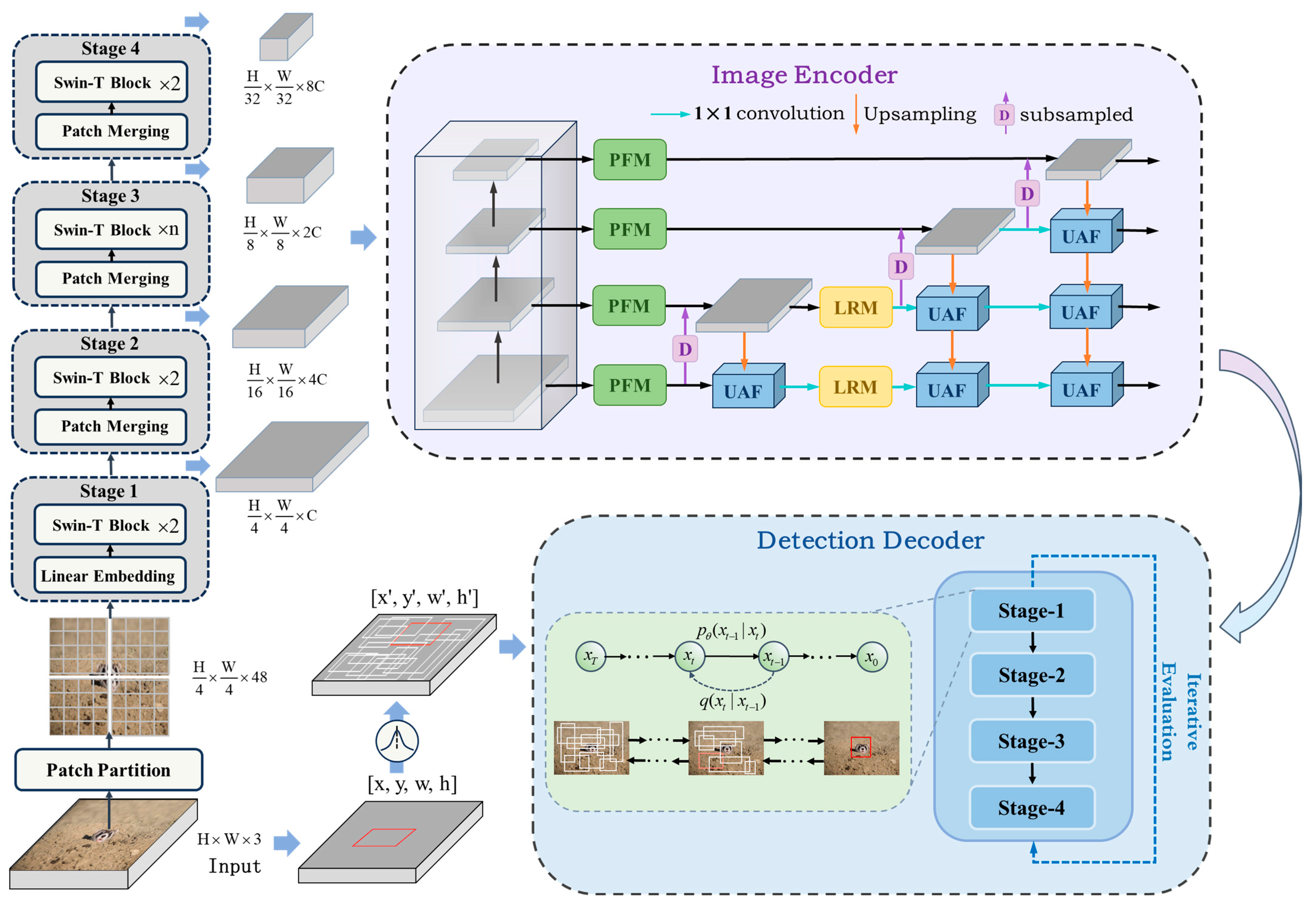
3.2. Proposed DMNet
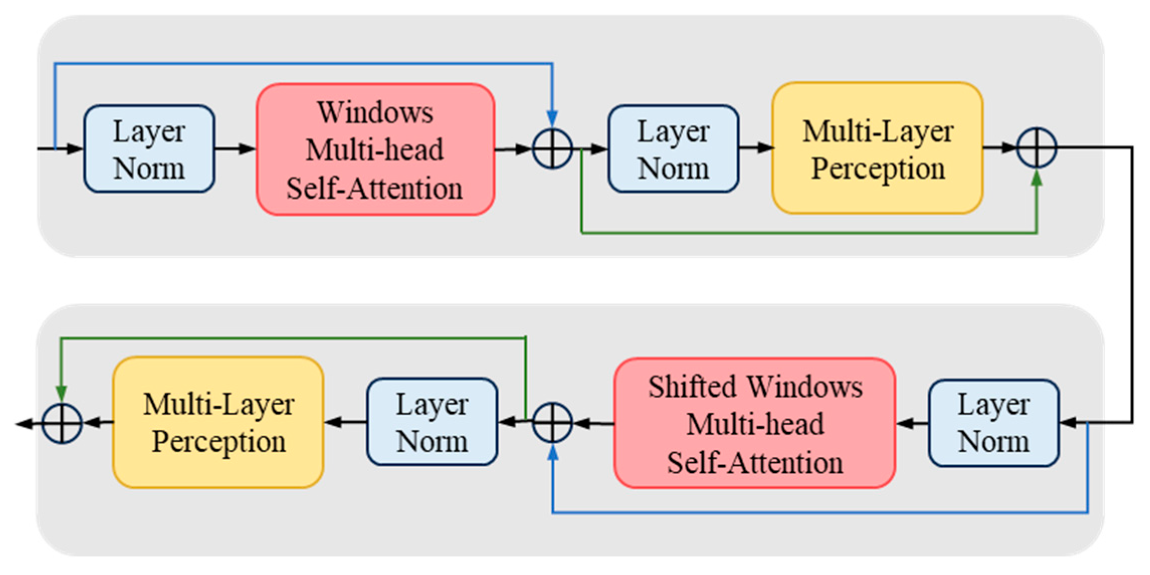
3.2.1. Feature Extraction Backbone
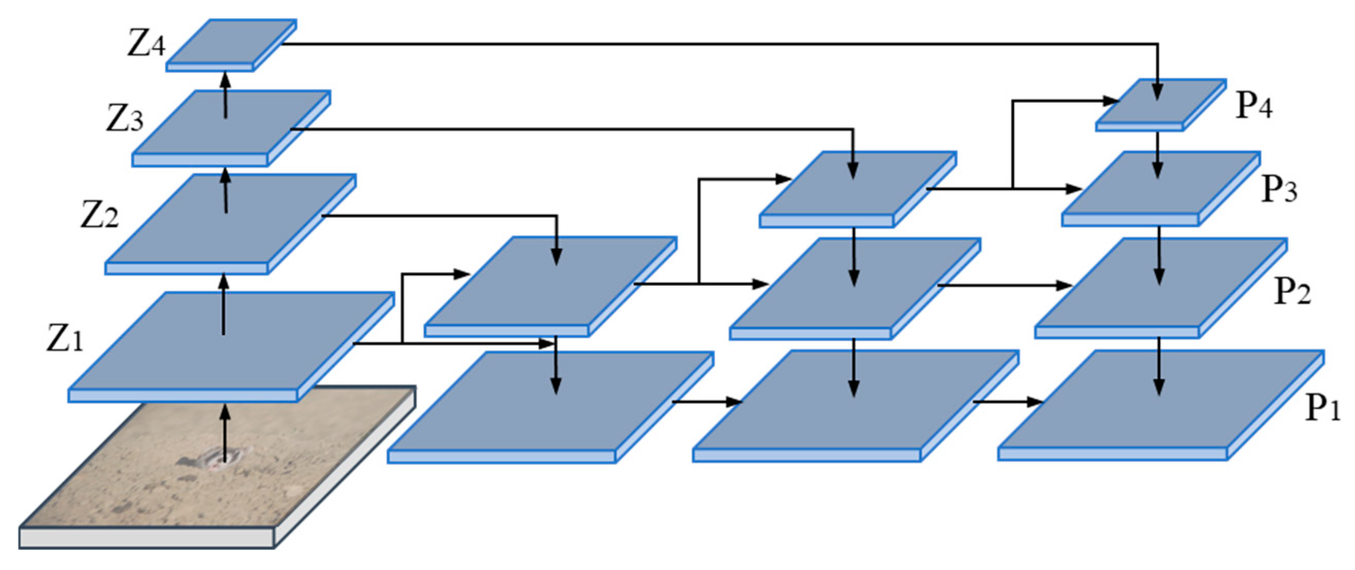
3.2.2. PFPN

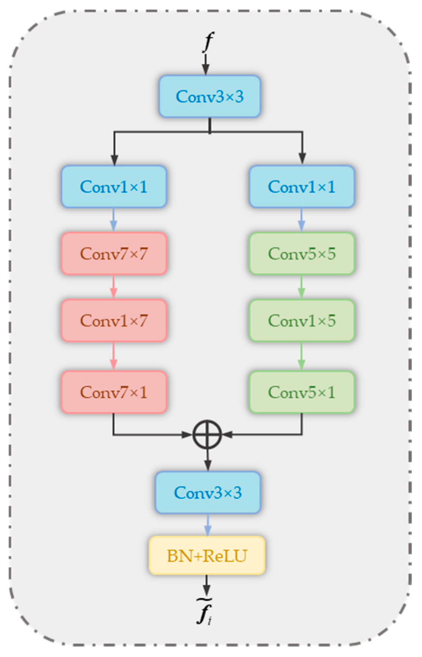
3.2.3. PFM
3.2.4. LRM

3.2.5. Detection Encoder

3.3. Training and Inference Strategies
3.3.1. Training Strategy
| Algorithm 1: Training Stage |
): = (B, N, 4) # B: batch # N: number of proposal boxes features = image_encoder (Images) ) for step, t in [T, …, 0]: eps = normal (mean = 0, std = 1) pb_crpt = sqrt((t)) pb + sqrt(1 − (t)) eps pb_pred = detection_decoder(pb_crpt, features, t) loss = pre_loss (pb_pred, GT_boxes) return loss |
3.3.2. Inference Strategy
| Algorithm 2: Inference Stage |
| Input: images, steps, T ddim_sampling (images, steps, T): # steps: number of sampling steps # T: time steps = normal (mean = 0, std = 1) times = reversed (linespace(−1, T, steps)) time_pairs = list (zip (times [: −1], times [1:])) :prediction boxes for t_now, t_next in zip(time_pairs): = detection_decoder (eps, features, t) , t_now, t_next) ) |
4. Results
4.1. Experimental Platform Configuration
4.2. Datasets and Evaluation Metrics
4.2.1. Dataset Settings
4.2.2. Evaluation Metrics
4.2.3. Training Settings
4.3. Loss Curves Experiments
4.4. Comparison Algorithms
4.5. Analysis of the Comparative Experimental Results
4.5.1. Quantitative Comparison
4.5.2. Qualitative Comparison
4.6. Ablation Experiments
4.7. Extended Experiments
5. Discussions
5.1. Advantages of DMNet
5.2. Limitations and Challenge
6. Conclusions
Author Contributions
Funding
Data Availability Statement
Conflicts of Interest
References
- Fan, D.P.; Ji, G.P.; Sun, G.; Cheng, M.M.; Shen, J.; Shao, L. Camouflaged object detection. In Proceedings of the 2020 IEEE/CVF conference on computer vision and pattern recognition (CVPR), Seattle, WA, USA, 13–19 June 2020; pp. 2774–2784. [Google Scholar]
- MacDonald, D.; Isenman, J.; Roman, J. Radar detection of hidden targets. In Proceedings of the IEEE 1997 National Aerospace and Electronics Conference (NAECON), Dayton, OH, USA, 14–17 July 1997; pp. 846–855. [Google Scholar]
- Gautam, A.K.; Preet, P.; Rawat, T.S.; Chowdhury, R.P.; Sinha, L.K. Detection of Camouflaged Targets in Hyperspectral Images; Springer: Singapore, 2020; pp. 155–161. [Google Scholar] [CrossRef]
- Shen, Y.; Lin, W.; Wang, Z.; Li, J.; Sun, X.; Wu, X.; Wang, S.; Huang, F. Rapid Detection of Camouflaged Artificial Target Based on Polarization Imaging and Deep Learning. IEEE Photonics J. 2021, 13, 1–9. [Google Scholar] [CrossRef]
- Felzenszwalb, P.F.; Girshick, R.B.; McAllester, D.A.; Ramanan, D. Object Detection with Discriminatively Trained Part Based Models. IEEE Trans. Pattern Anal. Mach Intell. 2010, 32, 1627–1645. [Google Scholar] [CrossRef] [PubMed]
- Redmon, J.; Divvala, S.K.; Girshick, R.B.; Farhadi, A. You Only Look Once: Unified; Real-Time Object Detection. In Proceedings of the 2016 IEEE Conference on Computer Vision and Pattern Recognition (CVPR), Las Vegas, NV, USA, 27–30 June 2016; pp. 779–788. [Google Scholar]
- Liu, W.; Anguelov, D.; Erhan, D.; Szegedy, C.; Reed, S.; Fu, C.Y.; Berg, A.C. SSD: Single Shot MultiBox Detector. In Proceedings of the Computer Vision–ECCV 2016, Amsterdam, The Netherlands, 11–14 October 2016; pp. 21–37. [Google Scholar]
- Tan, M.; Pang, R.; Le, Q.V. EfficientDet: Scalable and Efficient Object Detection. In Proceedings of the 2020 IEEE/CVF Conference on Computer Vision and Pattern Recognition (CVPR), Seattle, WA, USA, 13–19 June 2020; pp. 10778–10787. [Google Scholar]
- Sun, P.; Zhang, R.; Jiang, Y.; Kong, T.; Xu, C.; Zhan, W.; Tomizuka, M.; Li, L.; Yuan, Z.; Wang, C. Sparse R-CNN: End-to-End Object Detection with Learnable Proposals. In Proceedings of the 2021 IEEE/CVF Conference on Computer Vision and Pattern Recognition (CVPR), Nashville, TN, USA, 20–25 June 2021; pp. 14449–14458. [Google Scholar]
- Liu, Z.; Lin, Y.; Cao, Y.; Hu, H.; Wei, Y.; Zhang, Z.; Lin, S.; Guo, B. Swin Transformer: Hierarchical Vision Transformer using Shifted Windows. In Proceedings of the 2021 IEEE/CVF International Conference on Computer Vision (ICCV), Nashville, TN, USA, 20–25 June 2021; pp. 9992–10002. [Google Scholar]
- He, K.; Zhang, X.; Ren, S.; Sun, J. Spatial Pyramid Pooling in Deep Convolutional Networks for Visual Recognition. IEEE Trans. Pattern Anal. Mach Intell. 2014, 37, 1904–1916. [Google Scholar] [CrossRef] [PubMed]
- Wang, W.J.; Lu, Y.H.; Zheng, G.C.; Zhan, S.G.; Ye, X.Q.; Tan, Z.C.; Wang, J.D.; Wang, G.A.; Li, X. BEVSpread: Spread Voxel Pooling for Bird’s-Eye-View Representation in Vision-based Roadside 3D Object Detection. In Proceedings of the IEEE/CVF Conference on Computer Vision and Pattern Recognition (CVPR), Seattle, WA, USA, 17–21 June 2024; pp. 14718–14727. [Google Scholar]
- Tu, Y.; Zhang, B.; Liu, L.; Li, Y.; Chen, X.; Zhang, J.; Wang, Y.; Wang, C.; Zhao, C.R. Self-supervised Feature Adaptation for 3D Industrial Anomaly Detection. arXiv 2024, arXiv:2401.03145. [Google Scholar]
- la Fuente, R.P.-D.; Delclòs, X.; Peñalver, E.; Speranza, M.; Wierzchos, J.; Ascaso, C.; Engel, M.S. Early evolution and ecology of camouflage in insects. Proc. Natl. Acad. Sci. USA 2012, 109, 21414–21419. [Google Scholar] [CrossRef] [PubMed]
- Avrahami, O.; Lischinski, D.; Fried, O. Blended Diffusion for Text-driven Editing of Natural Images. arXiv 2022, arXiv:2111.14818. [Google Scholar]
- Wang, T.F.; Zhang, B.; Zhang, T.; Gu, S.Y.; Bao, J.M.; Baltrusaitis, T.; Shen, J.J.; Chen, D.; Wen, F.; Chen, Q.F.; et al. RODIN: A Generative Model for Sculpting 3D Digital Avatars Using Diffusion. In Proceedings of the 2023 IEEE/CVF Conference on Computer Vision and Pattern Recognition (CVPR), Vancouver, BC, Canada, 18–22 June 2023; pp. 4563–4573. [Google Scholar]
- Qian, H.; Huang, W.J.; Tu, S.K.; Xu, L. KGDiff: Towards explainable target-aware molecule generation with knowledge guidance. Brief Bioinform. 2023, 25, 435. [Google Scholar] [CrossRef] [PubMed]
- Esser, P.; Chiu, J.; Atighehchian, P.; Granskog, J.; Germanidis, A. Structure and Content-Guided Video Synthesis with Diffusion Models. In Proceedings of the 2023 IEEE/CVF International Conference on Computer Vision (ICCV), Paris, France, 2–6 October 2023; pp. 7312–7322. [Google Scholar]
- Chung, H.; Sim, B.; Ryu, D.; Ye, J.C. Improving Diffusion Models for Inverse Problems using Manifold Constraints. arXiv 2022, arXiv:2206.00941. [Google Scholar]
- Wu, J.; Fang, H.; Zhang, Y.; Yang, Y.; Xu, Y. MedSegDiff: Medical Image Segmentation with Diffusion Probabilistic Model. arXiv 2022, arXiv:2211.00611. [Google Scholar]
- Zhao, P.A.; Li, H.; Jin, R.Y.; Zhou, S.K. DiffULD: Diffusive Universal Lesion Detection. In Proceedings of the 26th International Conference on Vancouver, Vancouver, BC, Canada, 8–12 October 2023; pp. 94–105. [Google Scholar]
- Lv, W.; Huang, Y.; Zhang, N.; Lin, R.; Han, M.; Zeng, D. DiffMOT: A Real-time Diffusion-based Multiple Object Tracker with Non-linear Prediction. arXiv 2024, arXiv:2403.02075. [Google Scholar]
- Ding, X.H.; Guo, Y.C.; Ding, G.G.; Han, J.G. ACNet: Strengthening the Kernel Skeletons for Powerful CNN via Asymmetric Convolution Blocks. arXiv 2019, arXiv:1908.03930. [Google Scholar]
- Bolya, D.; Zhou, C.; Xiao, F.; Lee, Y.J. YOLACT: Real-Time Instance Segmentation. In Proceedings of the 2019 IEEE/CVF International Conference on Computer Vision (ICCV), Seoul, Republic of Korea, 27–28 October 2019; pp. 9156–9165. [Google Scholar]
- Cai, Z.; Vasconcelos, N. Cascade R-CNN: Delving Into High Quality Object Detection. In Proceedings of the 2018 IEEE/CVF Conference on Computer Vision and Pattern Recognition, Salt Lake City, UT, USA, 18–23 June 2018; pp. 6154–6162. [Google Scholar]
- Chen, H.; Sun, K.; Tian, Z.; Shen, C.; Huang, Y.; Yan, Y. BlendMask: Top-Down Meets Bottom-Up for Instance Segmentation. In Proceedings of the 2020 IEEE/CVF Conference on Computer Vision and Pattern Recognition (CVPR), Seattle, WA, USA, 13–19 June 2020; pp. 8570–8578. [Google Scholar]
- Zhang, S.; Chi, C.; Yao, Y.; Lei, Z.; Li, S. Bridging the Gap Between Anchor-Based and Anchor-Free Detection via Adaptive Training Sample Selection. In Proceedings of the 2020 IEEE/CVF Conference on Computer Vision and Pattern Recognition (CVPR), Seattle, WA, USA, 13–19 June 2020; pp. 9756–9765. [Google Scholar]
- Tian, Z.; Shen, C.; Chen, H. Conditional Convolutions for Instance Segmentation. In Proceedings of the Computer Vision–ECCV 2020, Glasgow, UK, 23–28 August 2020; pp. 282–298. [Google Scholar]
- Vu, T.; Kang, H.; Yoo, C.D. SCNet: Training Inference Sample Consistency for Instance Segmentation. Proc. AAAI Conf. Artif. Intell. 2021, 35, 2701–2709. [Google Scholar] [CrossRef]
- Feng, C.; Zhong, Y.; Gao, Y.; Scott, M.R.; Huang, W. TOOD: Task-aligned One-stage Object Detection. In Proceedings of the 2021 IEEE/CVF International Conference on Computer Vision (ICCV), Virtual, 11–17 October 2021; pp. 3490–3499. [Google Scholar]
- Zhang, H.; Wang, Y.; Dayoub, F.; Sunderhauf, N. VarifocalNet: An IoU-aware Dense Object Detector. In Proceedings of the 2021 IEEE/CVF Conference on Computer Vision and Pattern Recognition (CVPR), Nashville, TN, USA, 20–25 June 2021; pp. 8510–8519. [Google Scholar]
- Ke, L.; Danelljan, M.; Li, X.; Tai, Y.W.; Tang, C.K.; Yu, F. Mask Transfiner for High-Quality Instance Segmentation. In Proceedings of the 2022 IEEE/CVF Conference on Computer Vision and Pattern Recognition (CVPR), New Orleans, LA, USA, 19–20 June 2022. [Google Scholar]
- Duan, K.; Bai, S.; Xie, L.; Qi, H.; Huang, Q.; Tian, Q. CenterNet: Keypoint Triplets for Object Detection. In Proceedings of the 2019 IEEE/CVF International Conference on Computer Vision (ICCV), Seoul, Republic of Korea, 27–28 October 2019; pp. 6568–6577. [Google Scholar]
- Lee, Y.; Kim, J.; Willette, J.; Hwang, S.J. MPViT: Multi-Path Vision Transformer for Dense Prediction. In Proceedings of the 2022 IEEE/CVF Conference on Computer Vision and Pattern Recognition (CVPR), New Orleans, LA, USA, 19–20 June 2022; pp. 7277–7286. [Google Scholar]
- Zong, Z.F.; Song, G.L.; Liu, Y. DETRs with Collaborative Hybrid Assignments Training. In Proceedings of the IEEE/CVF International Conference on Computer Vision (ICCV), Paris, France, 2–6 October 2023; pp. 6725–6735. [Google Scholar]
- Zhang, H.; Li, F.; Liu, S.L.; Zhang, L.; Su, H.; Zhu, J.; Ni, L.M.; Shum, H.Y. DINO: DETR with Improved DeNoising Anchor Boxes for End-to-End Object Detection. arXiv 2022, arXiv:2203.03605. [Google Scholar]
- Jiang, X.H.; Cai, W.; Zhang, Z.L.; Jiang, B.; Yang, Z.Y.; Wang, X. Camouflaged object segmentation based on COSNet. Acta Arma. 2023, 44, 1456–1468. [Google Scholar]
- Lv, Y.; Zhang, J.; Dai, Y.; Li, A.; Liu, B.; Barnes, N. Simultaneously localize; segment and rank the camouflaged objects. In Proceedings of the 2021 IEEE/CVF Conference on Computer Vision and Pattern Recognition (CVPR), Nashville, TN, USA, 20–25 June 2021; pp. 11586–11596. [Google Scholar]


| Stage | AP50–95 | AP50 | AP75 | APS | APM | APL |
|---|---|---|---|---|---|---|
| 1 | 48.0 | 81.8 | 50.2 | 5.5 | 30.3 | 53.0 |
| 3 | 57.6 | 85.3 | 62.7 | 16.7 | 38.8 | 62.8 |
| 4 | 58.2 | 86.1 | 63.8 | 17.5 | 40.2 | 63.3 |
| 5 | 57.8 | 85.1 | 62.7 | 20.3 | 40.9 | 62.7 |
| 6 | 58.1 | 86.2 | 62.4 | 16.2 | 39.6 | 63.2 |
| Threshold | AP50–95 | AP50 | AP75 | APS | APM | APL |
|---|---|---|---|---|---|---|
| 0.30 | 56.3 | 83.7 | 61.6 | 16.4 | 39.2 | 61.2 |
| 0.35 | 56.6 | 84.8 | 61.2 | 17.1 | 39.3 | 61.5 |
| 0.40 | 57.1 | 85.3 | 61.9 | 14.8 | 39.0 | 62.2 |
| 0.50 | 51.0 | 80.8 | 54.1 | 18.5 | 34.4 | 55.7 |
| Names | Related Configurations |
|---|---|
| GPU | NVIDIA GeForce RTX 3090 |
| CPU | Xeon Gold 6148/128 G |
| GPU memory size | 24 G |
| Operating system | Win 10 |
| Computer platform | CUDA 12.2 |
| Deep learning framework | Pytorch |
| Iterations | AP50–95 | AP50 | AP75 | APS | APM | APL |
|---|---|---|---|---|---|---|
| 450,000 | 54.9 | 78.9 | 58.2 | 14.6 | 36.7 | 60.6 |
| 90,000 | 51.1 | 81.1 | 53.6 | 15.7 | 35.3 | 55.7 |
| 75,000 | 58.0 | 85.0 | 62.7 | 15.5 | 39.5 | 63.1 |
| 66,000 | 57.0 | 85.2 | 61.7 | 14.9 | 39.0 | 62.0 |
| 60,000 | 58.1 | 86.2 | 62.4 | 16.2 | 39.6 | 63.2 |
| 54,000 | 58.1 | 85.8 | 63.1 | 17.8 | 39.2 | 63.2 |
| 45,000 | 57.1 | 85.3 | 61.9 | 14.8 | 39.0 | 62.2 |
| Step | AP50–95 | AP50 | AP75 |
|---|---|---|---|
| 1 | 58.2 | 85.5 | 61.3 |
| 2 | 57.9 | 86.0 | 62.8 |
| 4 | 58.1 | 86.2 | 63.1 |
| 8 | 58.0 | 86.3 | 62.8 |
| Boxes | AP50–95 | AP50 | AP75 | Train-Duration |
|---|---|---|---|---|
| 200 | 50.9 | 79.6 | 54.1 | 8 h |
| 300 | 51.0 | 80.8 | 54.1 | 7.5 h |
| 500 | 50.5 | 81.0 | 52.9 | 12 h |
| 2000 | 50.4 | 81.1 | 54.0 | 23 h |
| Methods | Pub. Year | AP50–95 | AP50 | AP75 | APS | APM | APL |
|---|---|---|---|---|---|---|---|
| YOLACT [24] | ICCV2019 | 36.5 | 69.8 | 34.6 | 6.1 | 19.6 | 41.1 |
| Cascade RCNN [25] | TPAMI2019 | 46.3 | 73.5 | 48.4 | 8.4 | 27.9 | 51.4 |
| BlendMask [26] | CVPR2020 | 43.6 | 68.6 | 45.5 | 7.6 | 25.2 | 48.9 |
| ATSS [27] | ECCV2020 | 45.0 | 73.6 | 45.3 | 11.9 | 30.4 | 49.1 |
| CondInst [28] | ECCV2020 | 42.8 | 69.4 | 44.6 | 5.8 | 24.7 | 47.9 |
| SparseRCNN [9] | CVPR2021 | 46.5 | 74.9 | 47.9 | 12.4 | 34.3 | 50.4 |
| SCNet [29] | AAAI2021 | 47.1 | 75.5 | 48.2 | 13.8 | 29.0 | 52.0 |
| Swin-RCNN [10] | ICCV2021 | 50.2 | 79.8 | 54.6 | 11.3 | 31.9 | 55.3 |
| Tood [30] | ICCV2021 | 47.9 | 73.9 | 49.0 | 12.0 | 32.0 | 52.4 |
| VFNet [31] | CVPR2021 | 46.6 | 73.9 | 48.0 | 7.9 | 31.2 | 51.1 |
| MaskTrans [32] | CVPR2022 | 46.3 | 70.0 | 48.8 | 3.5 | 27.7 | 51.4 |
| Centernet [33] | Arxiv2022 | 42.3 | 72.3 | 42.2 | 11.0 | 24.7 | 47.3 |
| MPVIT-RCNN [34] | CVPR2022 | 57.8 | 82.3 | 63.3 | 17.2 | 38.1 | 62.9 |
| CO-DETR [35] | ECCV2023 | 44.5 | 63.5 | 32.3 | 8.3 | 20.9 | 37.4 |
| DINO [36] | ICLR2023 | 37.1 | 62.1 | 30.6 | 10.5 | 19.6 | 30.0 |
| DiffCOD | ours | 58.2 | 86.1 | 63.8 | 17.5 | 40.2 | 63.3 |
| Baseline | PFPN | PFM | LRM | DiffHead | AP50–95 | AP50 | AP75 | APS | APM | APL |
|---|---|---|---|---|---|---|---|---|---|---|
| 51.8 | 80.8 | 54.1 | 13.7 | 31.8 | 57.2 | |||||
| 57.5 | 83.4 | 62.1 | 10.5 | 39.5 | 61.6 | |||||
| 58.1 | 84.6 | 61.9 | 16.0 | 39.3 | 63.3 | |||||
| 58.1 | 84.2 | 62.4 | 16.2 | 39.6 | 62.4 | |||||
| 58.2 | 86.1 | 63.8 | 17.5 | 40.2 | 63.3 |
Disclaimer/Publisher’s Note: The statements, opinions and data contained in all publications are solely those of the individual author(s) and contributor(s) and not of MDPI and/or the editor(s). MDPI and/or the editor(s) disclaim responsibility for any injury to people or property resulting from any ideas, methods, instructions or products referred to in the content. |
© 2024 by the authors. Licensee MDPI, Basel, Switzerland. This article is an open access article distributed under the terms and conditions of the Creative Commons Attribution (CC BY) license (https://creativecommons.org/licenses/by/4.0/).
Share and Cite
Cai, W.; Gao, W.; Jiang, X.; Wang, X.; Di, X. Denoising Diffusion Implicit Model for Camouflaged Object Detection. Electronics 2024, 13, 3690. https://doi.org/10.3390/electronics13183690
Cai W, Gao W, Jiang X, Wang X, Di X. Denoising Diffusion Implicit Model for Camouflaged Object Detection. Electronics. 2024; 13(18):3690. https://doi.org/10.3390/electronics13183690
Chicago/Turabian StyleCai, Wei, Weijie Gao, Xinhao Jiang, Xin Wang, and Xingyu Di. 2024. "Denoising Diffusion Implicit Model for Camouflaged Object Detection" Electronics 13, no. 18: 3690. https://doi.org/10.3390/electronics13183690
APA StyleCai, W., Gao, W., Jiang, X., Wang, X., & Di, X. (2024). Denoising Diffusion Implicit Model for Camouflaged Object Detection. Electronics, 13(18), 3690. https://doi.org/10.3390/electronics13183690