
Real-Time Wild Horse Crossing Event Detection Using Roadside LiDAR


Abstract
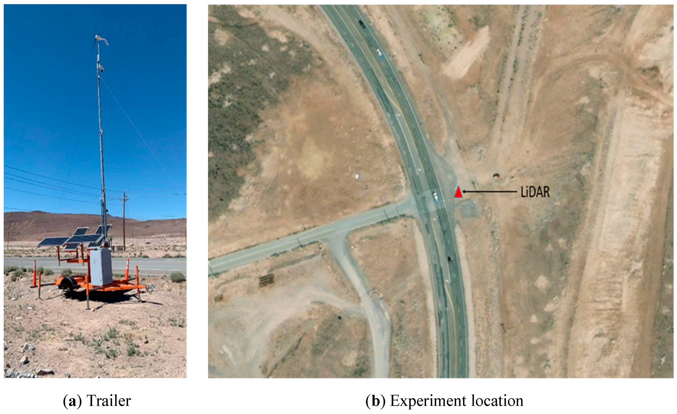
1. Introduction
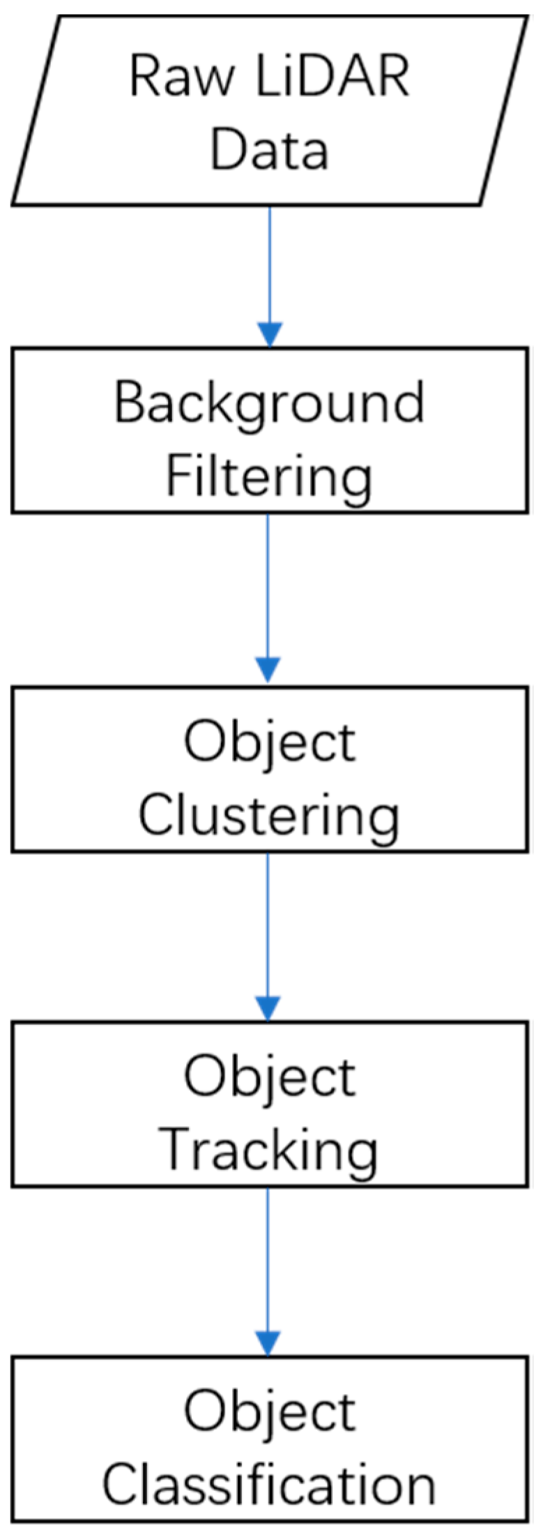
2. Methods
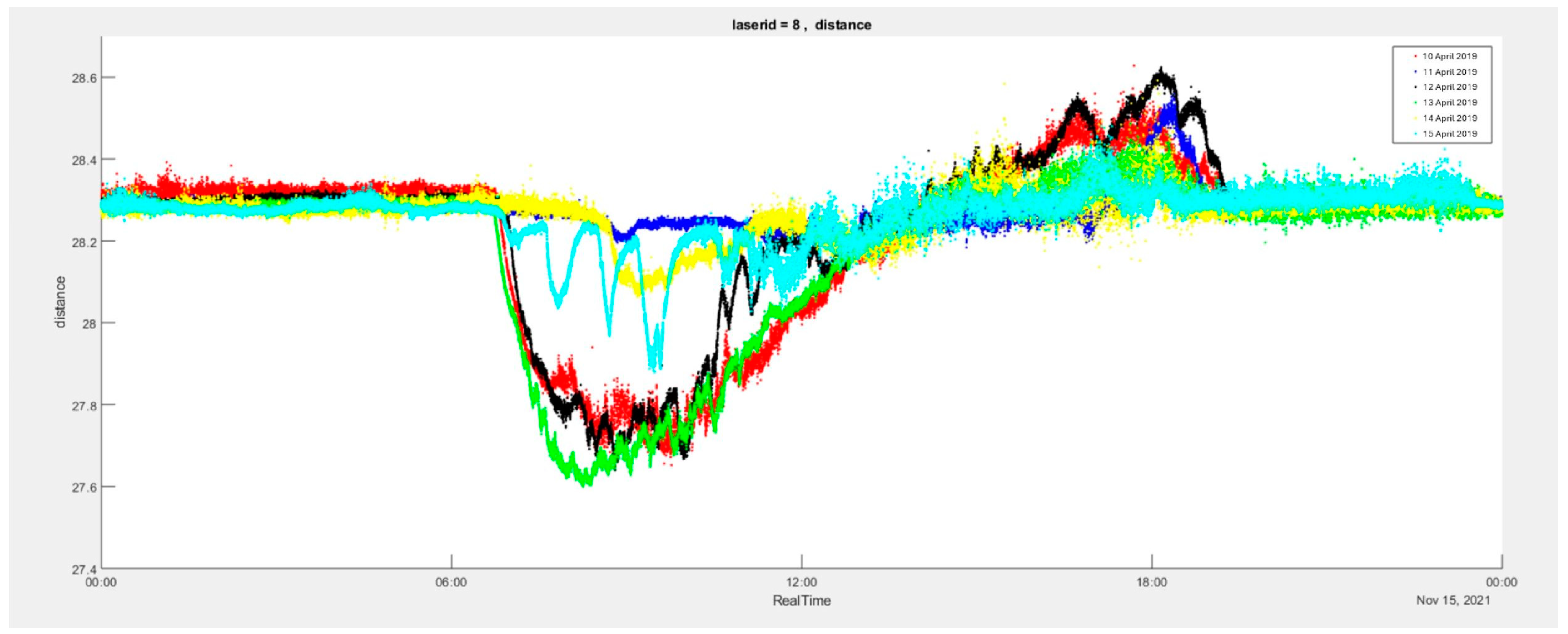
2.1. Background Filtering
2.2. Object Clustering
2.3. Object Tracking
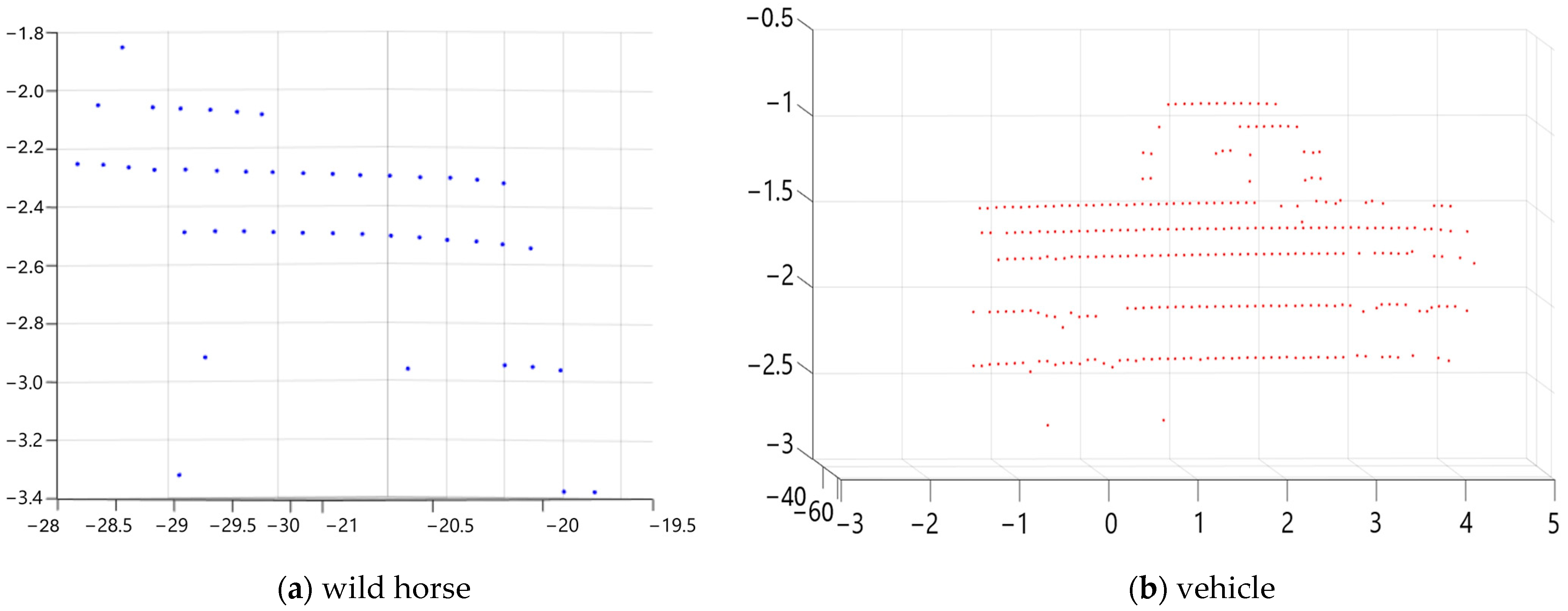
2.4. Object Classification
2.5. Classifier
2.6. Wild Horse Detection
3. Results
3.1. Parameter Setting
3.2. Model Evaluation
4. Conclusions
Author Contributions
Funding
Data Availability Statement
Conflicts of Interest
References
- Cramer, P.; McGinty, C. Prioritization of Wild Horse-Vehicle Conflict in Nevada; No. 604-16-803; Nevada Department of Transportation: Las Vegas, NV, USA, 2018.
- Huijser, M.P.; Kociolek, A.V.; McGowen, P.T.; Ament, R.; Hardy, A.; Clevenger, A.P.; Western Transportation Institute. Wildlife-Vehicle Collision and Crossing Mitigation Measures: A Toolbox for the Montana Department of Transportation; Montana Department of Transportation: Helena, MT, USA, 2007. [CrossRef]
- Benten, A.; Hothorn, T.; Vor, T.; Ammer, C. Wild horse warning reflectors do not mitigate wild horse–vehicle collisions on roads. Accid. Anal. Prev. 2018, 120, 64–73. [Google Scholar] [CrossRef] [PubMed]
- Ross, J.; Serpico, D.; Lewis, R. Assessment of Driver Yield Rates Pre-and Post-RRFB Installation, Bend, Oregon; No. FHWA-OR-RD 12-05; Transportation Research Section: Salem, OR, USA, 2011. [Google Scholar]
- Lu, X.; Lu, X. An efficient network for multi-scale and overlapped wild horse detection. Signal Image Video Process. 2023, 17, 343–351. [Google Scholar] [CrossRef]
- Nguyen, H.; Maclagan, S.J.; Nguyen, T.D.; Nguyen, T.; Flemons, P.; Andrews, K.; Ritchie, E.G.; Phung, D. Animal recognition and identification with deep convolutional neural networks for automated wild horse monitoring. In Proceedings of the 2017 IEEE International Conference on Data Science & Advanced Analytics, Tokyo, Japan, 19–21 October 2017. [Google Scholar]
- Feng, W.; Ju, W.; Li, A.; Bao, W.; Zhang, J. High-efficiency progressive transmission and automatic recognition of wild horse monitoring images with WISNs. IEEE Access 2019, 7, 161412–161423. [Google Scholar] [CrossRef]
- Rashed, H.; Ramzy, M.; Vaquero, V.; El Sallab, A.; Sistu, G.; Yogamani, S. Fusemodnet: Real-time camera and lidar based moving object detection for robust low-light autonomous driving. In Proceedings of the IEEE/CVF International Conference on Computer Vision Workshops, Seoul, Republic of Korea, 27–28 October 2019. [Google Scholar]
- Christiansen, P.; Steen, K.A.; Jørgensen, R.N.; Karstoft, H. Automated detection and recognition of wild horse using thermal cameras. Sensors 2014, 14, 13778–13793. [Google Scholar] [CrossRef] [PubMed]
- Viani, F.; Robol, F.; Giarola, E.; Benedetti, G.; De Vigili, S.; Massa, A. Advances in wild horse road-crossing early-alert system: New architecture and experimental validation. In Proceedings of the 8th European Conference on Antennas and Propagation (EuCAP 2014), The Hague, The Netherlands, 6–11 April 2014. [Google Scholar]
- Urbano, F.; Cagnacci, F. (Eds.) Spatial Database for GPS Wildlife Tracking Data: A Practical Guide to Creating a Data Management System with PostgreSQL/PostGIS and R, 2014th ed.; Springer: Cham, Switzerland; Berlin/Heidelberg, Germany, 2014. [Google Scholar]
- Ryota, R. Harmful Wild horse Detection System Utilizing Deep Learning for Radio Wave Sensing on Multiple Frequency Bands. In Proceedings of the 2019 International Conference on Artificial Intelligence in Information and Communication (ICAIIC), Okinawa, Japan, 11–13 February 2019. [Google Scholar]
- ALang, A.H.; Vora, S.; Caesar, H.; Zhou, L.; Yang, J.; Beijbom, O. PointPillars: Fast Encoders for Object Detection From Point Clouds. In Proceedings of the 2019 IEEE/CVF Conference on Computer Vision and Pattern Recognition (CVPR), Long Beach, CA, USA, 15–20 June 2019; pp. 12689–12697. [Google Scholar] [CrossRef]
- Zhou, Y.; Tuzel, O. VoxelNet: End-to-End Learning for Point Cloud Based 3D Object Detection. In Proceedings of the 2018 IEEE/CVF Conference on Computer Vision and Pattern Recognition (CVPR), Salt Lake City, UT, USA, 18–23 June 2018; pp. 4490–4499. [Google Scholar]
- Shi, S.; Wang, X.; Li, H. PointRCNN: 3D Object Proposal Generation and Detection From Point Cloud. In Proceedings of the 2019 IEEE/CVF Conference on Computer Vision and Pattern Recognition (CVPR), Long Beach, CA, USA, 15–20 June 2019; pp. 770–779. [Google Scholar]
- Zhang, C.; Chen, J.; Li, J.; Peng, Y.; Mao, Z. Large language models for human–robot interaction: A review. Biomim. Intell. Robot. 2023, 3, 100131. [Google Scholar] [CrossRef]
- Arfaoui, A. Unmanned aerial vehicle: Review of onboard sensors, application fields, open problems and research issues. Int. J. Image Process 2017, 11, 12–24. [Google Scholar]
- Guan, F.; Xu, H.; Tian, Y. Evaluation of Roadside LiDAR-Based and Vision-Based Multi-Model All-Traffic Trajectory Data. Sensors 2023, 23, 537. [Google Scholar] [CrossRef] [PubMed]
- Wu, J.; Xu, H.; Zheng, Y.; Zhang, Y.; Lv, B.; Tian, Z. Automatic Vehicle Classification using Roadside LiDAR Data. Transp. Res. Rec. J. Transp. Res. Board 2019, 2673, 153–164. [Google Scholar] [CrossRef]
- Lv, B.; Xu, H.; Wu, J.; Tian, Y.; Zhang, Y.; Zheng, Y.; Yuan, C.; Tian, S. LiDAR-Enhanced Connected Infrastructures Sensing and Broadcasting High-Resolution Traffic Information Serving Smart Cities. IEEE Access 2019, 7, 79895–79907. [Google Scholar] [CrossRef]
- Wu, J.; Xu, H.; Zheng, Y.; Tian, Z. A novel method of vehicle-pedestrian near-collision identification with roadside LiDAR data. Accid. Anal. Prev. 2018, 121, 238–249. [Google Scholar] [CrossRef] [PubMed]
- Zhang, Z.; Zheng, J.; Wang, X.; Fan, X. Background filtering and vehicle detection with roadside lidar based on point association. In Proceedings of the 2018 37th Chinese Control Conference (CCC), Wuhan, China, 25–27 July 2018. [Google Scholar]
- Wu, J.; Xu, H.; Zheng, J. Automatic background filtering and lane identification with roadside LiDAR data. In Proceedings of the 2017 IEEE 20th International Conference on Intelligent Transportation Systems (ITSC), Yokohama, Japan, 16–19 October 2017. [Google Scholar]
- Zhang, T.; Jin, P.J. Roadside LiDAR Vehicle detection and tracking using range and intensity background subtraction. J. Adv. Transp. 2022, 2022, 2771085. [Google Scholar] [CrossRef]
- Bäcklund, H.; Hedblom, A.; Neijman, N. A density-based spatial clustering of application with noise. Data Min. 2011, 33, 11–30. [Google Scholar]
- Qi, Y.; Yao, H.; Sun, X.; Sun, X.; Zhang, Y.; Huang, Q. Structure-aware multi-object discovery for weakly supervised tracking. In Proceedings of the 2014 IEEE International Conference on Image Processing (ICIP), Paris, France, 27–30 October 2014; pp. 466–470. [Google Scholar] [CrossRef]
- Ge, C.; Song, Y.; Ma, C.; Qi, Y.; Luo, P. Rethinking Attentive Object Detection via Neural Attention Learning. IEEE Trans. Image Process. 2023, 33, 1726–1739. [Google Scholar] [CrossRef] [PubMed]
- Yang, Y.; Li, G.; Qi, Y.; Huang, Q. Release the Power of Online-Training for Robust Visual Tracking. In Proceedings of the AAAI Conference on Artificial Intelligence, New York, NY, USA, 7–12 February 2020; Volume 34, pp. 12645–12652. [Google Scholar] [CrossRef]
- Qi, Y.; Qin, L.; Zhang, S.; Huang, Q.; Yao, H. Robust visual tracking via scale-and-state-awareness. Neurocomputing 2018, 329, 75–85. [Google Scholar] [CrossRef]
- Zhao, J.; Xu, H.; Wu, D.; Liu, H. An artificial neural network to identify pedestrians and vehicles from roadside 360-degree LiDAR data. In Proceedings of the 97th Annual Transportation Research Board Meeting, Washington, DC, USA, 11–17 January 2018. [Google Scholar]
- Lee, H.; Coifman, B. Side-fire lidar-based vehicle classification. Transp. Res. Rec. J. Transp. Res. Board 2012, 2308, 173–183. [Google Scholar] [CrossRef]


| Average Error Rate | Last Day Error Rate | |
|---|---|---|
| Error Type 1 | 3.2% | 1.7% |
| Error Type 2 | 2.0% | 1.8% |
| DT | |||
| Real | Wild horse | Others | |
| Predict | |||
| Wild horse | 4741 | 231 | |
| Others | 172 | 4260 | |
| NB | |||
| Real | Wild horse | Others | |
| Predict | |||
| Wild horse | 4633 | 389 | |
| Others | 280 | 4102 | |
| KNN | |||
| Real | Wild horse | Others | |
| Predict | |||
| Wild horse | 3857 | 753 | |
| Others | 1056 | 3738 | |
| SVM | |||
| Real | Wild horse | Others | |
| Predict | |||
| Wild horse | 4898 | 256 | |
| Others | 15 | 4235 | |
| Recall | Precision | |
|---|---|---|
| PointPillars [13] | 90.2% | 82.3% |
| Our method | 99.6% | 95.0% |
| Detected Time | Detected Frame | Start Position | End Position |
|---|---|---|---|
| 30 April 2022 3:00 | 8773–10,610 | (75.9, −54.7) | (35.7, 40.7) |
| 30 April 2022 7:00 | 4941–5226 | (−21.1, −56.9) | (−25.9, −15.7) |
| 25 April 2022 11:00 | 1665–2749 | (70.4, −77.6) | (84.2, −77.3) |
| 25 April 2022 18:30 | 15,728–17,999 | (−35.4, −24.9) | (−54.1, −64.0) |
| 25 April 2022 7:00 | 2–1310 | (17.2, 36.2) | (34.0, 39.0) |
| 25 April 2022 7:30 | 2–937 | (70.7, 12.0) | (91.9, −50.7) |
Disclaimer/Publisher’s Note: The statements, opinions and data contained in all publications are solely those of the individual author(s) and contributor(s) and not of MDPI and/or the editor(s). MDPI and/or the editor(s) disclaim responsibility for any injury to people or property resulting from any ideas, methods, instructions or products referred to in the content. |
© 2024 by the authors. Licensee MDPI, Basel, Switzerland. This article is an open access article distributed under the terms and conditions of the Creative Commons Attribution (CC BY) license (https://creativecommons.org/licenses/by/4.0/).
Share and Cite
Wang, Z.; Xu, H.; Guan, F.; Chen, Z. Real-Time Wild Horse Crossing Event Detection Using Roadside LiDAR. Electronics 2024, 13, 3796. https://doi.org/10.3390/electronics13193796
Wang Z, Xu H, Guan F, Chen Z. Real-Time Wild Horse Crossing Event Detection Using Roadside LiDAR. Electronics. 2024; 13(19):3796. https://doi.org/10.3390/electronics13193796
Chicago/Turabian StyleWang, Ziru, Hao Xu, Fei Guan, and Zhihui Chen. 2024. "Real-Time Wild Horse Crossing Event Detection Using Roadside LiDAR" Electronics 13, no. 19: 3796. https://doi.org/10.3390/electronics13193796
APA StyleWang, Z., Xu, H., Guan, F., & Chen, Z. (2024). Real-Time Wild Horse Crossing Event Detection Using Roadside LiDAR. Electronics, 13(19), 3796. https://doi.org/10.3390/electronics13193796