Robust Adaptive Sliding Mode Control Using Stochastic Gradient Descent for Robot Arm Manipulator Trajectory Tracking

Abstract

This paper presents an innovative control strategy for robot arm manipulators, utilizing an adaptive sliding mode control with stochastic gradient descent (ASMCSGD). The ASMCSGD controller significant improvements in robustness, chattering elimination, and fast, precise trajectory tracking. Its performance is systematically compared with super twisting algorithm (STA) and conventional sliding mode control (SMC) controllers, all optimized using the grey wolf optimizer (GWO). Simulation results show that the ASMCSGD controller achieves root mean squared errors (RMSE) of $0.12758$ for ${\theta }_1$ and $0.13387$ for ${\theta }_2$. In comparison, the STA controller yields RMSE values of $0.1953$ for ${\theta }_1$ and $0.1953$ for ${\theta }_2$, while the SMC controller results in RMSE values of $0.24505$ for ${\theta }_1$ and $0.29112$ for ${\theta }_2$. Additionally, the ASMCSGD simplifies implementation, eliminates unwanted oscillations, and achieves superior tracking performance. These findings underscore the ASMCSGD’s effectiveness in enhancing trajectory tracking and reducing chattering, making it a promising approach for robust control in practical applications of robot arm manipulators.

1. Introduction

Recently, robot manipulators have been used to replace human efforts in hazardous [1] or repetitive tasks such as welding [2], painting [3], deburring [4], material handling [5], and many other assembly operations [6]. The size and complexity of these manipulators depend on their intended use and the work envelope of the manipulator. Depending on the reference frames of the workpiece, tasks of a predetermined nature can be selected, comprising the control of the end-effector, e.g., in Cartesian axes for correcting task positioning and orientation in space or the joint axes for performing path following of trajectories. With the necessity of increasing the number of movements that the manipulator can do to develop more complicated tasks, multiple robot configurations or more than one robot arm configuration is being increasingly used, and the development works have been carried out, mainly focusing on the control and path planning aspects [7].

Many control techniques have been developed to address the challenges posed by these increasingly complex manipulator configurations. Trajectory tracking control, in particular, has seen significant advancements by applying various methodologies. Traditional approaches like proportional-integral-derivative (PID) control remain widely used due to their simplicity and effectiveness in a range of scenarios [8,9,10]. However, as tasks grow in complexity, more sophisticated techniques such as sliding mode control (SMC) have gained traction, offering robustness against nonlinearities and external disturbances [11,12,13].

To further enhance control performance, fuzzy logic controllers (FLC) have been employed, providing a way to handle the uncertainties and imprecision inherent in real-world robotic systems [14,15,16]. These controllers excel in scenarios where conventional control methods might struggle. Additionally, neural networks (NNs) have been integrated into control systems to provide adaptive capabilities, enabling robotic arms to learn and adjust their behavior in real-time [17]. This approach is particularly effective when combined with SMC or FLC, forming hybrid control strategies that capitalize on the strengths of each method [18,19,20]. In more recent developments, these advanced control techniques have been used in conjunction with trajectory tracking algorithms, ensuring that the robotic arms can precisely follow complex paths even in dynamic and unpredictable environments. The integration of adaptive learning algorithms, such as SGD, within these control frameworks further optimizes performance, allowing the system to improve and adapt to the changing conditions [21] continually.

However, these techniques have been applied in numerous studies and applications; for instance, Majed et al. [22] highlighted the widespread use of PID controllers across various levels of industrial automation, ranging from small-scale industries to advanced technological applications. In their study, they focused on designing a position controller for a robot arm by optimizing PID parameters using a genetic algorithm (GA). They modeled the robot arm as a third-order system and compared two PID tuning methods: one utilizing genetic algorithms and the other based on the Ziegler–Nichols (ZN) method. Their findings demonstrated that the PID parameters optimized through the GA outperformed those tuned by the ZN method, indicating that the proposed approach could be effectively extended to higher-order systems as well. Bingol et al. [23] proposed that the Scorbot ER-V Plus robot arm is modeled in the SolidWorks environment, and the 3D solid model is converted into SimMechanics format. The robot’s electric motor is controlled using a PID controller with a low-pass filter (LPF). The controller parameters are optimized using a sinusoidal reference signal and external disturbances that account for total uncertainties, including parameter variations and load torque. Inverse kinematics are applied to determine the joint angles from the specified trajectory, and these angles are used to achieve the desired trajectory. The optimized controller demonstrates good and robust control performance. As Zhao et al. [24] proposed, to address the challenges of strong coupling and nonlinearity in the robot arm control system, a fuzzy PID controller optimized by GA. This approach effectively controls nonlinear systems by leveraging an FLC strategy, which enhances the system’s dynamic response speed and adaptive capability. The GA is employed to optimize and self-tune the PID control parameters, using the overall performance index as the fitness function. This optimization compensates for the low precision typically associated with FLC. In the context of robot arm control, the fuzzy PID controller, with parameters optimized by the GA, demonstrates fast response and minimal overshoot. Moreover, the system shows a certain degree of adaptability in the face of external disturbances and parameter variations. Simulation results confirm the effectiveness and practicality of this algorithm, suggesting its applicability to other control systems and processes.

The use of SMC as a robust control strategy for robotic systems is due to its effectiveness in handling nonlinearities, uncertainties, and external disturbances. The SMC forces the system’s state trajectory to reach and stay on a predefined sliding surface, ensuring that the robot arm achieves the desired motion with high accuracy and robustness. Numerous research studies have applied this type of control to enhance the performance of robotic systems. For instance, Pan et al. [25] proposed that compliant actuators are vital for safe human-robot interaction. They developed a compact series elastic actuator (SEA) that provides high force control fidelity and low output impedance. Their study focused on controlling a robot arm driven by this SEA. The control problem is addressed as a singularly perturbed system with slow rigid robot dynamics and fast SEA dynamics. A second-order sliding mode control (SO-SMC) law is used to achieve precise tracking with minimal chattering, ensuring semi-global exponential stability for the rigid robot dynamics. A derivative-type control law is employed for the global exponential stability of the SEA dynamics. This work represents the first use of continuous SMC in robots with compliant actuators, with experimental results demonstrating high-accuracy tracking performance. Zakia et al. [26] proposed an SMC for their study; they explored a hybrid control scheme combining SMC with traditional PID control for a 2-DoF planar manipulator. Since PID control does not require precise system modeling, they designed the sliding mode surface using the PID component parameters of the manipulator. The PID control adjusts the system errors within the closed loop, while the SMC ensures rapid convergence to the sliding mode surface. This hybrid approach leverages the strengths of both control schemes, resulting in enhanced system stability. Eltayeb et al. [27] proposed an adaptive sliding mode control (ASMC) strategy for a multi-input, multi-output (MIMO) robotic arm nonlinear manipulator system. Their controller, designed using the Lyapunov theorem, aims to achieve robust trajectory tracking while addressing system uncertainties and mitigating the chattering issue commonly associated with traditional sliding mode control. Their results indicated that the proposed ASMC controller maintains robust performance in trajectory tracking despite parameter uncertainties and significantly reduces chattering. Zhang et al. [28] introduced a torque tracking control method utilizing a dual surface sliding mode controller (DSSMC) to enhance performance for a 2-DoF robotic arm. Unlike traditional approaches where desired torques are fixed or sinusoidal, their method calculates the torques automatically based on the Lagrange equations. The robotic arm, which comprises an upper arm and a back arm, is driven by two electrohydraulic servo systems (EHSS). The DSSMC approach employs two sliding surfaces and variable structure control laws to achieve precise torque tracking. Compared with conventional PID controllers and standard SMCs, the DSSMC significantly reduces torque tracking overshoot and greatly improves tracking accuracy.

On the other hand, FLCs and NNs offer distinct advantages for robotic arm control over conventional controllers. The FLC handles complex and nonlinear dynamics using heuristic rules, providing flexibility and robustness against uncertainties and disturbances. Hence, NNs, through their learning and adaptive capabilities, excel in modeling intricate relationships and optimizing control strategies based on real-world data, making them well-suited for high-dimensional and sophisticated control tasks. Both methods reduce dependence on precise system modeling, enhancing adaptability, accuracy, and overall control performance in dynamic environments, thus offering significant improvements over PID and SMC approaches. For example, in Jouila et al. [29] proposed a robust adaptive control method for a 2-DoF robotic manipulator that enhances tracking performance despite dynamic uncertainties and disturbances. Their approach uses a non-singular fast time sliding mode (NFTSM) controller combined with a wavelet neural network (WNN) to estimate uncertainties and disturbances. This method includes a compensation term to reduce the effects of approximation errors and disturbances, improving tracking accuracy and reducing chattering. Controller parameters are tuned online using an adaptive learning algorithm, with control laws based on the Lyapunov stability theorem. Simulations demonstrate that this approach significantly improves performance compared with other advanced control strategies. Bi [9] proposed a control algorithm that utilizes symmetry principles to enhance fault diagnosis and optimize performance for robot arms. The approach incorporates an optimized fuzzy PID algorithm, which adjusts the PID gains based on error rates. The focus is on designing a control system for a 2-DoF manipulator, a complex MIMO nonlinear system. The study begins by establishing the mathematical model of the 2-DoF articulated manipulator, defining the relationship between the input driving force vector and the output rotation angle vector. Trajectory planning algorithms are then developed using gradient model control to determine the end-effector’s path according to specific task requirements. Experimental results demonstrate the effectiveness of this control approach in terms of speed response and small error tracking.

Hybrid controllers, which combine conventional control methods with advanced techniques, offer significant advantages in controlling complex systems like robotic arms. These controllers leverage the strengths of different approaches, such as the stability and simplicity of classical controllers and the adaptability and robustness of more advanced methods. By integrating these techniques, hybrid controllers can better handle nonlinearity, uncertainties, and dynamic changes in the system. This combination allows for enhanced precision, improved response to disturbances, and greater overall control performance, making them a powerful tool for achieving reliable and efficient operation in a wide range of applications. For instance, Efe [11] proposed a novel approach to enhance the robustness of fuzzy SMC by incorporating an adaptive neuro-fuzzy inference system (ANFIS) architecture. This method introduces fractional-order integration during the parameter tuning phase, ensuring that the control system is directed toward the sliding regime in the traditional sense. Compared with the classical integer-order approach, the proposed scheme demonstrates superior tracking performance, along with heightened robustness and insensitivity to disturbances. These benefits are substantiated through simulations using the dynamic model of a 2-DoF direct-drive robot arm. Their study highlights that the system’s response is significantly improved when fractional-order integration is applied in the parameter adaptation stage, compared with the classical integer-order integration method. Bikova et al. [15] proposed a rajectory-tracking algorithm for a 2-DoF robotic arm using FLC, each designed for a specific joint. Unlike conventional methods, this approach uses position, velocity, and acceleration as inputs. The study emphasizes its potential application in medical robotics, particularly for heart surgery. Simulation results in MATLAB/Simulink show that the algorithm performs effectively across various input signals, with a focus on sinusoidal tracking, demonstrating robust performance. Mohan et al. [30] proposed a versatile 2-DoF fractional order fuzzy PI-D (2-DoF FOFPI-D) controller designed for a class of nonlinear systems. This control scheme is derived from a basic 2-DoF fractional order PID controller in the discrete domain, incorporating expert intelligence through a formula-based fuzzy design methodology. The controller structure includes a fractional order fuzzy PI (FOFPI) and a fractional order derivative filter, providing flexibility in design and a self-tuning control feature. The proposed approach is compared with its integer-order counterpart and a 2-DoF PI-D controller for a coupled nonlinear 2-link robotic arm in a real-world operating environment. The controller parameters are optimally tuned using a multi-objective, non-dominated sorting genetic algorithm (II), aimed at minimizing variations in control effort and error index. Extensive simulation studies evaluate the controller’s performance in trajectory tracking, handling model uncertainties, cogging disturbances, sensor noise, and disturbance rejection. The results demonstrate that the 2-DoF FOFPI-D controller outperforms the other controllers under various operating conditions.

1.1. Contributions

This paper investigates the comparative performance of an adaptive sliding mode control using stochastic gradient descent (ASMCSGD) against traditional SMC and STA controllers. The ASMCSGD controller offers the advantage of adapting the SMC gain using gradient descent, which simplifies implementation, eliminates unwanted oscillations, and achieves high and fast performance tracking. Additionally, it ensures high robustness under noisy conditions. The controller’s parameters are tuned in real-time to adapt to changes in system dynamics, uncertainties, or disturbances, maintaining optimal performance and robustness in dynamic and uncertain environments.

1.2. Structure Overview

The remainder of this paper is structured as follows: Section 2 offers an in-depth discussion of the dynamic modeling of a 2-DoF robotic manipulator. Section 3 explains the principles and implementation of the control strategies. Section 4 presents the simulation results. Finally, the paper concludes with a summary of the contributions and a conclusion in the final section.

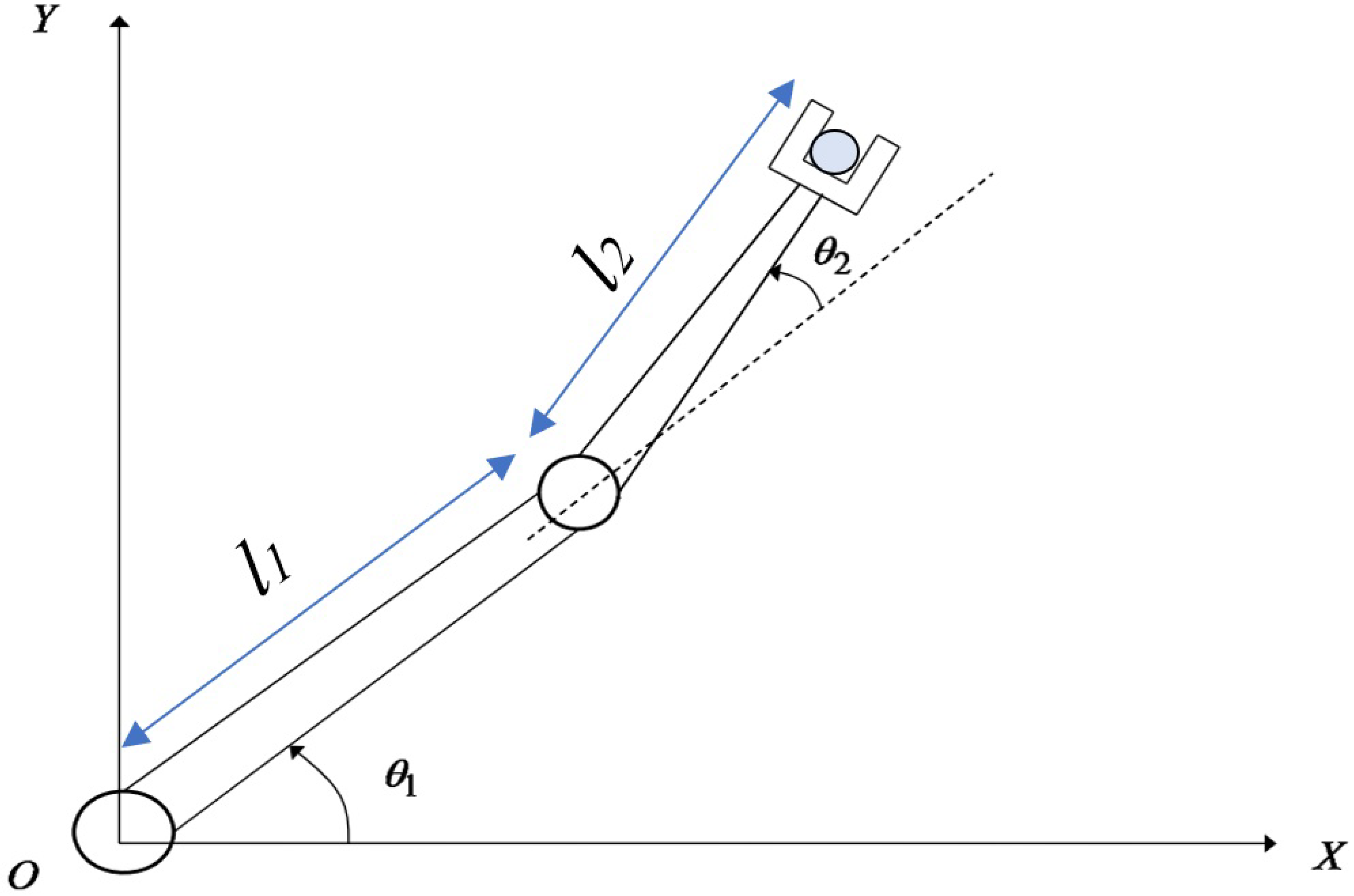
2. Dynamic Modeling of a 2-DoF Robot Arm Manipulator

As shown in Figure 1, a two-degrees-of-freedom (2-DoF) robot arm consists of two rigid links with $l_1$ and $l_2$ lengths. The 2-DoF can have different configurations, depending on the lengths of the links. For example, a two-link may have its second link endpoint moving on a circle when the lengths of the links $l_1$ and $l_2$ are equal. If $l_2$ is greater than $l_1$, the second link endpoint will trace an ellipse. In another case, when $l_1$ = $l_2$, a two-link robot is equivalent to the parallelogram linkage, and its second endpoint traces a straight line path [31]. Thus, for a 2-DoF planar robot, its endpoint path can be predicted when its dimensions are known. The dynamic model for the 2-DoF robot arm manipulator can be presented by the following equation [32,33]:

$$I\left(q\right)\ddot{q}+C(q,\dot{q})\dot{q}+G\left(q\right)=\tau$$

(1)

In this context, q, $\dot{q}$ and $\ddot{q}\in {\mathbb{R}}^2$ represent the vectors of joint angles, joint velocities, and joint accelerations, respectively. The inertia matrix is denoted by $I\left(q\right)\in {\mathbb{R}}^{2\times 2}$, while $C(q,\dot{q})\in {\mathbb{R}}^2$ represents the Coriolis and centrifugal matrix and $G\left(q\right)\in {\mathbb{R}}^2$ is the gravitational vector. The vector of joint torques is given by $\tau \in {\mathbb{R}}^2$. The specific forms of the matrices $I\left(q\right)$, $C(q,\dot{q})$ and $G\left(q\right)$ are provided in Appendix A. Accordingly, the equation can be rearranged as follows [34]:

$$\ddot{q}=-I^{-1}C(q,\dot{q})\dot{q}-I^{-1}\left(q\right)G\left(q\right)+I^{-1}\left(q\right)\tau$$

(2)

The dynamic equation governing the motion of the 2-DoF robot manipulator can be expressed in a compact form as follows:

$$\ddot{q}=-\gamma \dot{q}-\beta G\left(q\right)+\beta u\left(t\right)$$

(3)

In this context, $\gamma =I^{-1}C(q,\dot{q})$, $\beta =I^{-1}\left(q\right)$, and $u\left(t\right)=\tau$ denote the control vector. To account for variations in system parameters, parameter uncertainties are introduced, resulting in the following modified equation [35]:

$$\ddot{q}=-(\gamma +\delta \gamma )\dot{q}-(\beta +\delta \beta )G\left(q\right)+(\beta +\delta \beta )u\left(t\right)$$

(4)

where $\delta \gamma$ and $\delta \beta$ represent the uncertainties in the parameters. This equation can be further rewritten as

$$\ddot{q}=-\gamma \dot{q}-\beta G\left(q\right)+\beta u\left(t\right)+d\left(t\right)$$

(5)

where $d\left(t\right)=-\delta \gamma \dot{q}-\delta \beta G\left(q\right)+\delta \beta u\left(t\right)$. Following the definition of the disturbance term $d\left(t\right)$, the tracking error is expressed as follows:

$$e\left(t\right)=q\left(t\right)-q_d\left(t\right)$$

(6)

where $q\left(t\right)$ denotes the actual system state and $q_d\left(t\right)$ represents the desired trajectory. The error $e\left(t\right)$ characterizes the deviation of the system state from the reference trajectory.

3. Control Design

This section presents the implementation of an adaptive sliding mode control using stochastic gradient descent (ASMCSGD) for a 2-DoF robotic arm, as illustrated in Figure 2. The ASMCSGD controller operates within a proportional-derivative (PD) surface, which is utilized for the entire set of proposed controllers. The PD surface is selected to minimize steady-state error, while the derivative term enhances transient response, resulting in improved overall tracking performance. The ASMCSGD approach introduces adaptive gains that can be adjusted via stochastic gradient descent (SGD) and a learning rate, $\mu$. The use of SGD aims to refine and adapt the SMC, thereby enhancing its effectiveness and reducing the chattering. Moreover, this approach allows the controller parameter to be tuned in real-time to adapt to changes in system dynamics, uncertainties, or disturbances, maintaining optimal performance and robustness. The SGD is preferred over other methods due to its efficiency and quicker convergence in real-time applications. In addition, SGD updates parameters incrementally based on immediate feedback, which results in improved tracking precision, reduced oscillations, and enhanced robustness under noisy conditions.

3.1. Sliding Mode Control

The sliding mode control (SMC) guarantees that the states will converge to the origin within a finite time, offering enhanced tracking performance and faster convergence. The general surface can be described as follows [36]:

$$s_c=K_{p}e+K_d\dot{e}$$

(7)

where $K_p$ is a $2\times 2$ diagonal matrix representing positive proportional gains and $K_d$ is a $2\times 2$ diagonal matrix representing positive derivative gains, both of which must be selected for the 2-DoF robotic manipulator. The SMC method aims to drive the tracking error toward the sliding surface and then maintain it on this surface until it reaches its origin. In order to ensure that the error decreases asymptotically, the sliding surface must be stable, meaning ${lim}_{t\to \infty }e\left(t\right)=0$. Taking the time derivative of the general sliding surface and using Equations (5) and (6) yields

$$\begin{array}{c}{\dot{s}}_c=K_p\dot{e}+K_d\ddot{e}\hfill \\ =K_p\dot{e}+K_d\left[-\gamma \dot{q}-\beta G\left(q\right)+\beta u-{\ddot{q}}_d+d\left(t\right)\right]\hfill \end{array}$$

(8)

In order to achieve the condition where $\dot{s}=0$, the standard equivalent control is calculated as follows:

$$u_{seq}={\left(K_d\beta \right)}^{-1}\left[-K_p\dot{e}+K_d\gamma \dot{q}+K_d\beta G+K_d{\ddot{q}}_d\right]$$

(9)

However, this equivalent control might not guarantee optimal performance, particularly in the presence of unexpected disturbances such as parameter changes or external load variations. To ensure the system meets the reaching condition, an additional control component, known as the switching or reaching control, denoted as $u_{s1}$ for the first controller (SMC), is required. The switching control law $u_{s1}$ is defined as

$$u_{s1}=-k_s·\mathrm{sign}\left(s_c\right)$$

(10)

where $k_s$ is a positive constant. The complete SMC law is then given by

$$u_1=u_{seq}+u_{s1}$$

(11)

To ensure that the tracking position error progresses smoothly from the reaching phase to the sliding phase, a Lyapunov stability criterion is introduced as follows [37]:

$$V\left(s_c\right)={\displaystyle \frac{1}{2}}{s}_c^T{s}_c$$

(12)

Taking the time derivative of the Lyapunov function results in

$$\dot{V}\left(s_c\right)={\displaystyle \frac{d}{dt}}\left({\displaystyle \frac{1}{2}}{s}_c^T{s}_c\right)=s_c^T\dot{s_c}$$

(13)

Substituting Equations (8)–(11) into Equation (13) gives

$$\begin{array}{ccc}\hfill \dot{V}\left(s_c\right)=s_c^T\dot{s_c}& =& s_c^T\left[K_p\dot{e}+K_d\ddot{e}\right]\hfill \\ & =& s_c^T\left[K_p\dot{e}+K_d(\ddot{q}-{\ddot{q}}_d)\right]\hfill \\ & =& s^T\left[K_p\dot{e}+K_d(-\gamma \dot{q}-\beta G)\right]\hfill \\ & +& s_c^T\left[K_d\beta (u_{seq}+u_{s1})-K_d{\ddot{q}}_d+K_{d}d\left(t\right)\right]\hfill \\ & =& s_c^T\left[K_p\dot{e}-K_d\gamma \dot{q}-K_d\beta G\right]\hfill \\ & +& s_c^T\left[K_d\beta u_{seq}+K_d\beta u_{s1}-K_d{\ddot{q}}_d+K_{d}d\left(t\right)\right]\hfill \end{array}$$

(14)

Given that $u_{seq}$ cancels the corresponding terms in $\dot{s_c}$, simplifying Equation (14) results in

$$\dot{V}\left(s_c\right)=s_c^T\dot{s_c}=s_c^T\left(-K_d\beta ·k_s·\mathrm{sign}\left(s_c\right)+K_{d}d\left(t\right)\right)$$

(15)

Since $s_c^T·\mathrm{sign}\left(s_c\right)=\left|s_c\right|$, this reduces to

$$\dot{V}\left(s_c\right)=-K_d\beta ·k_s·\left|s_c\right|+s_c^T{K}_{d}d\left(t\right)$$

(16)

As $K_d$, $\beta$ and $k_s$ are positive, $\dot{V}\left(s_c\right)$ remains negative as $s_c$ approaches zero if $k_s$ is greater than d(t)/$\beta$. Therefore, according to Equation (7), the error converges to zero, confirming the controller’s stability.

3.2. Super Twisting Control

The super twisting algorithm (STA) combined with a PD sliding surface is an advanced control technique that enhances robustness and reduces chattering in SMC [38]. The STA is ensures that the sliding variable $s_c$ converges to zero in finite time, providing robustness against uncertainties and disturbances. In order to implement the STA, the general second control form is defined as follows [39]:

$$u_2=u_{seq}+u_{s2}$$

(17)

where the equivalent control $u_{seq}$ is taken by the same for the previous SMC which is defined in Equation (9). The STA control law is given by [40]

$$u_{s2}=-{\lambda }_1·sign\left(s_c\right)·{\left|s_c\right|}^{0.5}-{\lambda }_2·\int sign\left(s_c\right)dt$$

(18)

where ${\lambda }_1$ and ${\lambda }_2$ are positive constants. Using Equations (7), (9), (17), and (18) and substituting into Equation (8) yields

$$\begin{array}{cc}\dot{s_c}\hfill & =K_p\dot{e}+K_d\left[-\gamma \dot{q}-\beta G\left(q\right)+\beta \left(u_{seq}+u_{s2}\right)+d\left(t\right)-{\ddot{q}}_d\right]\hfill \\ \hfill & =-K_d\beta \left({\lambda }_1·\mathrm{sign}\left(s_c\right){\left|s_c\right|}^{0.5}+{\lambda }_2·\int \mathrm{sign}\left(s_c\right)dt\right)\hfill \\ \hfill & =-K_d\beta {\lambda }_1·\mathrm{sign}\left(s_c\right){\left|s_c\right|}^{0.5}-K_d\beta {\lambda }_2·\int \mathrm{sign}\left(s_c\right)dt\hfill \end{array}$$

(19)

By definition, $K_d\beta {\lambda }_1=K_1$ and $K_d\beta {\lambda }_2=K_2$, where $K_1$ and $K_2$ are positive constants. Now let $\xi$$=-K_2·\int \mathrm{sign}\left(s_c\right)$; therefore, Equation (19) can be expressed as follows:

$${\dot{s}}_c=-K_1·\mathrm{sign}\left(s_c\right)·{\left|s_c\right|}^{0.5}+\xi$$

(20)

$$\dot{\xi }=-K_2·\mathrm{sign}\left(s_c\right)$$

(21)

Finite-time convergence and robustness of the STA have been established through geometric approaches and the homogeneity properties of the algorithm, as discussed by Moreno and Osorio [41]. It is clear that $s_c=0$ and $\dot{s_c}=0$ are achieved when the variables s and $\delta$ converge to zero within a finite time $t_s$ [41]. Consequently, the SMC is attained after $t_s=t$. The reduction in chattering is as described by Equation (20). To validate this, it is necessary to demonstrate the convergence of the variables s and $\xi$ to zero. Moreno and Osorio [41] provided proof of this convergence. The relevant results from their work are summarized in the following theorem:

Theorem 1.

The following statements are equivalent:

• The origin $x=0$ of Equations (20) and (21) is finite-time stable.
• The matrix $A=\left[\begin{array}{cc}-{\displaystyle \frac{1}{2}}{K}_1& {\displaystyle \frac{1}{2}}\\ -K_2& 0\end{array}\right]$ is Hurwitz, meaning all its eigenvalues have negative real parts.
• The constant gains $K_1$ and $K_2$ are positive, i.e., $K_1>0$ and $K_2>0$.
• For every symmetric and positive definite matrix $Q=Q^T>0$, the Algebraic Lyapunov Equation (ALE) $A^{T}P+PA=-Q$ has a unique symmetric and positive definite solution $P=P^T>0$.

In this scenario, the function $V\left(x\right)$, defined as $V\left(x\right)={\xi }^{T}P\xi$, acts as a global, strict Lyapunov function for the system. This is true for any $P=P^T>0$ that satisfies the ALE with a given positive definite matrix $Q=Q^T>0$ [41]. Consequently, by choosing $K_1$ and $K_2$ in the control law of Equation (18) to be positive, sliding surface can be achieved. If the sliding surfaces is designed to match the original SMC, then once the sliding mode is reached, the system performance will be equivalent to that under SMC [42].

3.3. Adaptive Sliding Mode Using Stochastic Gradient Descent

The SGD is an optimization algorithm used to minimize a function by iteratively moving in the direction of the steepest descent (Figure 3), which is the negative gradient of the function [43]. The primary goal of SGD is to find the minimum value of a cost function or loss function, which quantifies the error between the predicted and actual values in a such model [43]. Hence, within the SMC, SGD is utilized to adaptively tune the controller gain. By incorporating SGD, the controller gain is dynamically adjusted based on real-time feedback, enhancing the system performance and robustness.

In order to implement the SMC using the SGD algorithm, an adaptive control signal $u_{ad}$ should be deduced. Hence, the complete adaptive control law using adaptive SMC is formulated as follows:

$$u_{ad}=u_{seq}+u_{s3}$$

(22)

where the equivalent control is defined in (9), while the conventional switching control is provided as follows:

$$u_{s3}=-k_{ad}\left(t\right)·\mathrm{sign}\left(s_c\right)$$

(23)

where $k_{ad}\left(t\right)$ represents the adaptive gain associated with the ASMCSGD controller. To define the adaptive gain, the objective function is expressed as follows [43]:

$${\mathcal{L}}_{gr}={\displaystyle \frac{1}{2}}{\left(e_{gr}\right)}^2={\displaystyle \frac{1}{2}}{(u_{ref}-u_{ad})}^2$$

(24)

where $e_{gr}$ represents the gradient error. The following equation describes the parameter update for the SMC controller using the SGD method [44]:

$${\dot{k}}_{ad}\left(t\right)=-\mu .{\displaystyle \frac{\delta {\mathcal{L}}_{gr}}{\delta k_{ad}\left(t\right)}}$$

(25)

where $\mu \in (0,1)$ is the adaptive rate [44]. Equation (25) can be expressed by the following formula:

$${\displaystyle \frac{\delta {\mathcal{L}}_{gr}}{\delta k_{ad}\left(t\right)}}={\displaystyle \frac{\delta {\mathcal{L}}_{gr}}{\delta u_{ad}}}.{\displaystyle \frac{\delta u_{ad}}{\delta k_{ad}\left(t\right)}}$$

(26)

Using Equations (22) and (24), the derivative terms of Equation (26) can be expressed as follows:

$$\left\{\begin{array}{c}{\displaystyle \frac{\delta {\mathcal{L}}_{gr}}{\delta u_{ad}}}=u_{ad}-u_{ref}\hfill \\ {\displaystyle \frac{\delta u_{ad}}{\delta k_{ad}\left(t\right)}}=-\mathrm{sign}\left(s_c\right)\hfill \end{array}\right.$$

(27)

Therefore, by substituting formulas of Equation (27) into Equation (25), then the adaptive gain $k_{ad}\left(t\right)$ can be expressed as follows:

$$k_{ad}\left(t\right)=-\mu \int \left[(u_{ad}-u_{ref})\left(\mathrm{sign}\left(s_c\right)\right)\right]dt$$

(28)

where $u_{ref}$ is the reference control input that represents the desired ideal control signal for the system. The complete adaptive control is defined by Equation (29).

$$u_{ad}={\left(K_d\beta \right)}^{-1}\left[-K_p\dot{e}+K_d\gamma \dot{q}+K_d\beta G+K_d{\ddot{q}}_d-K_{d}d\left(t\right)\right]-k_{ad}\left(t\right)·\mathrm{sign}\left(s_c\right)$$

(29)

To establish the stability of the ASMCSGD, a Lyapunov function is proposed for the system dynamics as follows:

$$V\left(s_c\right)={\displaystyle \frac{1}{2}}{s}_c^T{s}_c$$

(30)

By taking the time derivative, the Lyapunov function results in

$$\dot{V}\left(s_c\right)={\displaystyle \frac{d}{dt}}\left({\displaystyle \frac{1}{2}}{s}_c^T{s}_c\right)=s_c^T\dot{s_c}$$

(31)

In order to demonstrate the proposed ASMCSGD controller stability, the system dynamics are considered. Therefore, by applying Equations (8), (9), (22), (23) and (25) yield:

$$\begin{array}{ccc}\hfill \dot{V}\left(s_c\right)=s_c^T\dot{s_c}& =& s_c^T\left[K_p\dot{e}+K_d\ddot{e}\right]\hfill \\ & =& s_c^T\left[K_p\dot{e}+K_d(\ddot{q}-{\ddot{q}}_d)\right]\hfill \\ & =& s_c^T\left[K_p\dot{e}+K_d(-\gamma \dot{q}-\beta G)\right]\hfill \\ & +& s_c^T\left[K_d\beta (u_{seq}+u_{s3})-K_d{\ddot{q}}_d+K_{d}d\left(t\right)\right]\hfill \\ & =& s_c^T\left[K_p\dot{e}-K_d\gamma \dot{q}-K_d\beta G\right]\hfill \\ & +& s_c^T\left[K_d\beta u_{seq}+K_d\beta u_{s3}-K_d{\ddot{q}}_d+K_{d}d\left(t\right)\right]\hfill \\ & =& s_c^T\left(-K_d\beta ·k_{ad}\left(t\right)·\mathrm{sign}\left(s_c\right)+K_{d}d\left(t\right)\right)\hfill \\ & =& -K_d\beta ·k_{ad}\left(t\right)·\left|s_c\right|+s_c^T{K}_{d}d\left(t\right)\hfill \end{array}$$

(32)

Taking into account that $K_p$, $K_d$, and $\beta$ are positive and assuming that $k_{ad}$ is greater than d(t)/$\beta$. Then, according to the Lyapunov theory, the proposed control scheme is stable. In order to enhance the proposed controllers’ gains, a GWO is used, which is described in the next section.

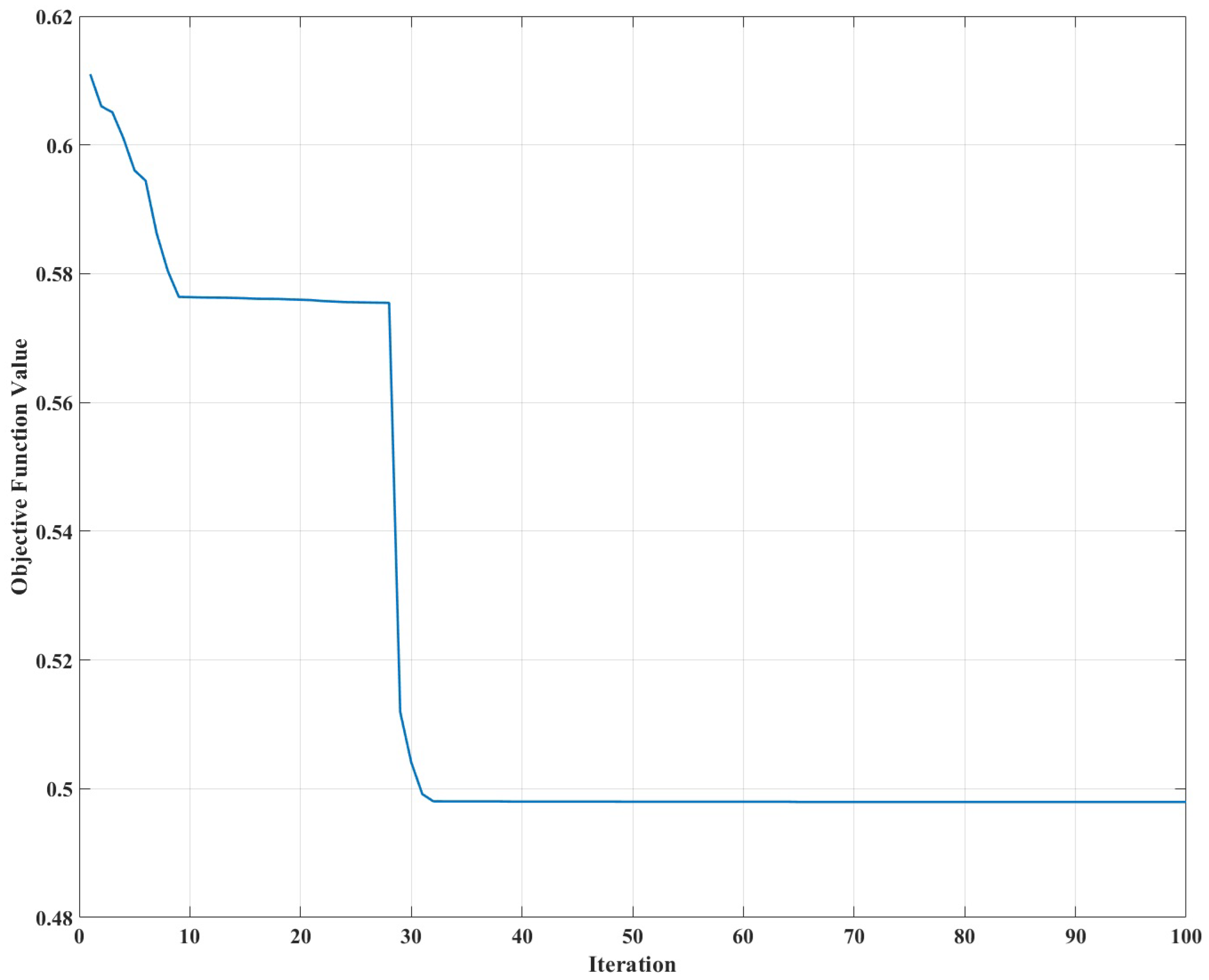
4. The Grey Wolf Optimizer

The grey wolf optimizer (GWO) is a metaheuristic optimization technique inspired by the leadership and hunting behaviors of grey wolves. Introduced by Mirjalili et al. [45]. in 2014, this algorithm has gained recognition for its simplicity and effectiveness across various optimization challenges. In GWO, wolves are divided into four categories: $\alpha$, $\beta$, $\delta$, and $\omega$, with $\alpha$ denoting the best solution, followed by $\beta$, $\delta$, and $\omega$, which represent the remaining search agents. The algorithm emulates the wolves’ hunting process through three key phases [45].

4.1. Encircling the Prey

The behavior of encircling the prey is represented by the following equations [46]:

$$\mathbf{D}=\left|\mathbf{C}·{\mathbf{X}}_p\left(t\right)-\mathbf{X}\left(t\right)\right|$$

(33)

$$\mathbf{X}(t+1)={\mathbf{X}}_p\left(t\right)-\mathbf{A}·\mathbf{D}$$

(34)

where the following is true:

• $\mathbf{D}$ denotes the distance vector between the current position of the wolf and the prey.
• ${\mathbf{X}}_p$ represents the position vector of the prey.
• $\mathbf{X}$ indicates the position vector of the grey wolf.
• t refers to the current iteration.
• $\mathbf{A}$ and $\mathbf{C}$ are coefficient vectors computed as follows:

$$\mathbf{A}=2\mathbf{a}·{\mathbf{r}}_1-\mathbf{a}$$

(35)

$$\mathbf{C}=2·{\mathbf{r}}_2$$

(36)

In these equations, $\mathbf{a}$ decreases linearly from 2 to 0 throughout the iterations, while ${\mathbf{r}}_1$ and ${\mathbf{r}}_2$ are random vectors within the range $[0,1]$.

4.2. Hunting

Following the encircling phase, the wolves move to the hunting phase, guided by the alpha ($\alpha$), beta ($\beta$) and delta ($\delta$) wolves, who lead the pack. The distance vectors from each wolf to these leaders are calculated as follows [46,47]:

$${\mathbf{D}}_{\alpha }=\left|{\mathbf{C}}_1·{\mathbf{X}}_{\alpha }-\mathbf{X}\right|,$$

(37)

$${\mathbf{D}}_{\beta }=\left|{\mathbf{C}}_2·{\mathbf{X}}_{\beta }-\mathbf{X}\right|,$$

(38)

$${\mathbf{D}}_{\delta }=\left|{\mathbf{C}}_3·{\mathbf{X}}_{\delta }-\mathbf{X}\right|,$$

(39)

where ${\mathbf{X}}_{\alpha }$, ${\mathbf{X}}_{\beta }$ and ${\mathbf{X}}_{\delta }$ denote the positions of the alpha, beta and delta wolves, respectively. The coefficient matrices ${\mathbf{C}}_1$, ${\mathbf{C}}_2$ and ${\mathbf{C}}_3$ adjust the influence of each leader. Each wolf updates its position using the positions and distances from these leaders:

$${\mathbf{X}}_1={\mathbf{X}}_{\alpha }-{\mathbf{A}}_1·{\mathbf{D}}_{\alpha },$$

(40)

$${\mathbf{X}}_2={\mathbf{X}}_{\beta }-{\mathbf{A}}_2·{\mathbf{D}}_{\beta },$$

(41)

$${\mathbf{X}}_3={\mathbf{X}}_{\delta }-{\mathbf{A}}_3·{\mathbf{D}}_{\delta },$$

(42)

and then averages these updated positions to determine its new position:

$$\mathbf{X}(t+1)={\displaystyle \frac{{\mathbf{X}}_1+{\mathbf{X}}_2+{\mathbf{X}}_3}{3}}.$$

(43)

4.3. Attacking the Prey

In the final phase, referred to as the attack on prey, the wolves focus on converging towards the optimal solution identified by the alpha, beta, and delta leaders. During this phase, the exploration capability, denoted by the parameter $\mathbf{a}$, is progressively reduced with each iteration. This reduction shifts the focus from exploring new regions to intensively searching around the best solutions discovered so far. By decreasing $\mathbf{a}$, the algorithm enhances the exploitation phase, allowing for finer tuning and better optimization in the vicinity of the most promising solutions identified by the pack leaders. The flowchart of the GWO optimization method is illustrated in Figure 4.

In this paper, the GWO plays a crucial role in optimizing the performance of the ASMCSGD controller. While ASMCSGD adapts control gains and the learning rate in real-time, determining optimal parameters is vital for improving tracking accuracy and minimizing chattering. The GWO is employed in order to automate this optimization process, ensuring that control gains and the learning rate are fine-tuned for optimal performance. By leveraging GWO’s exploration and exploitation capabilities, the ASMCSGD controller benefits from globally optimized parameters, which enhance robustness, stability, and tracking performance.

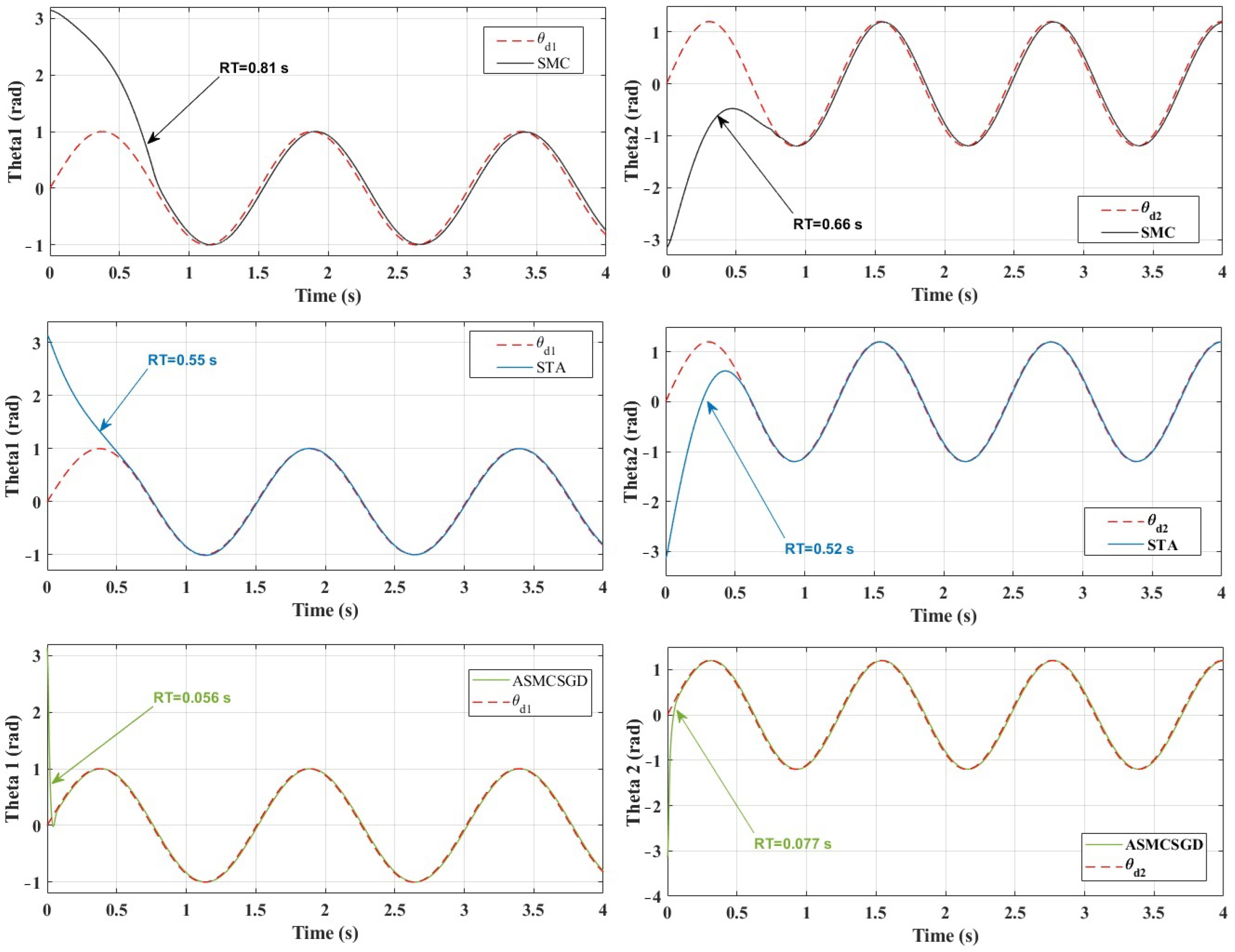
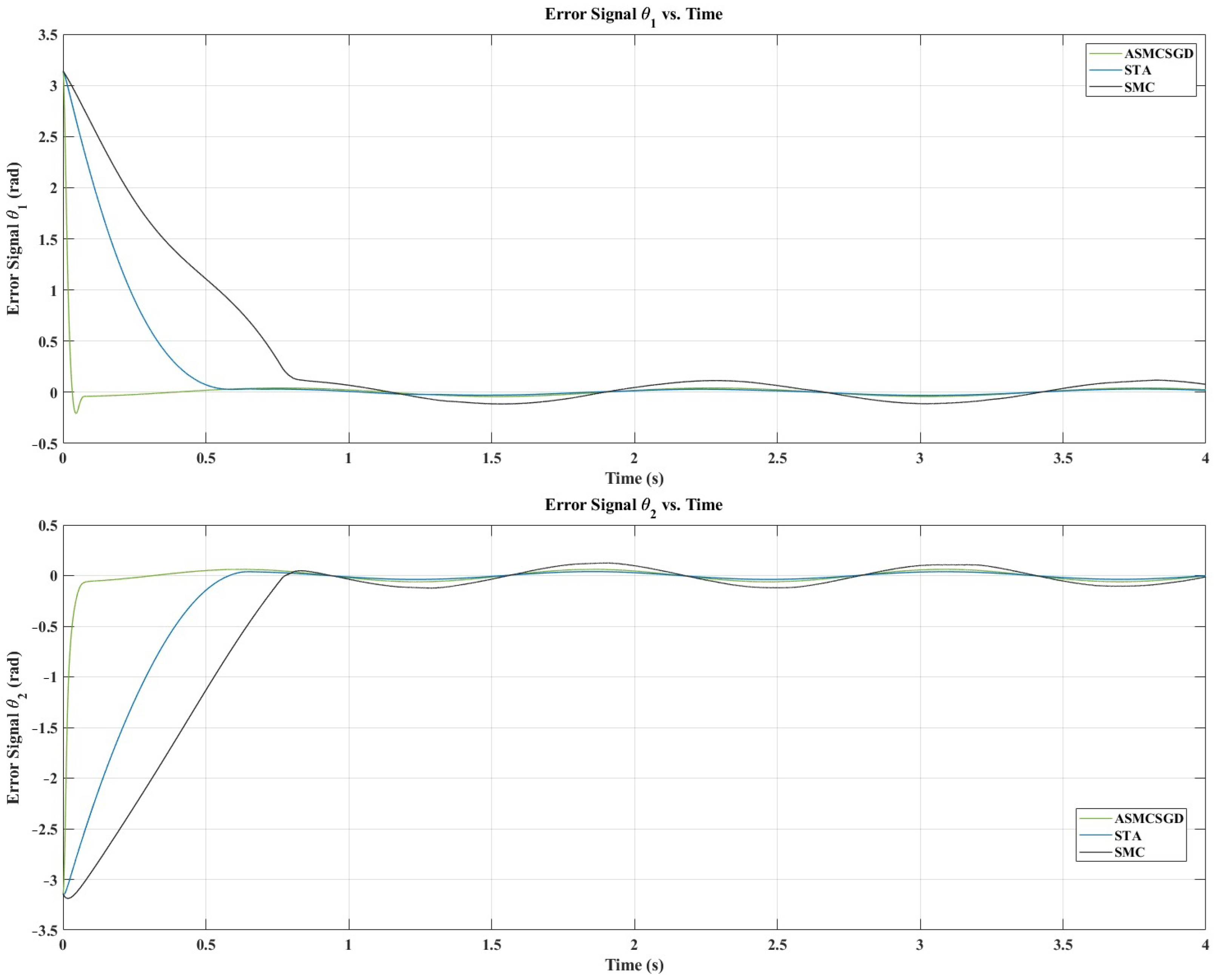
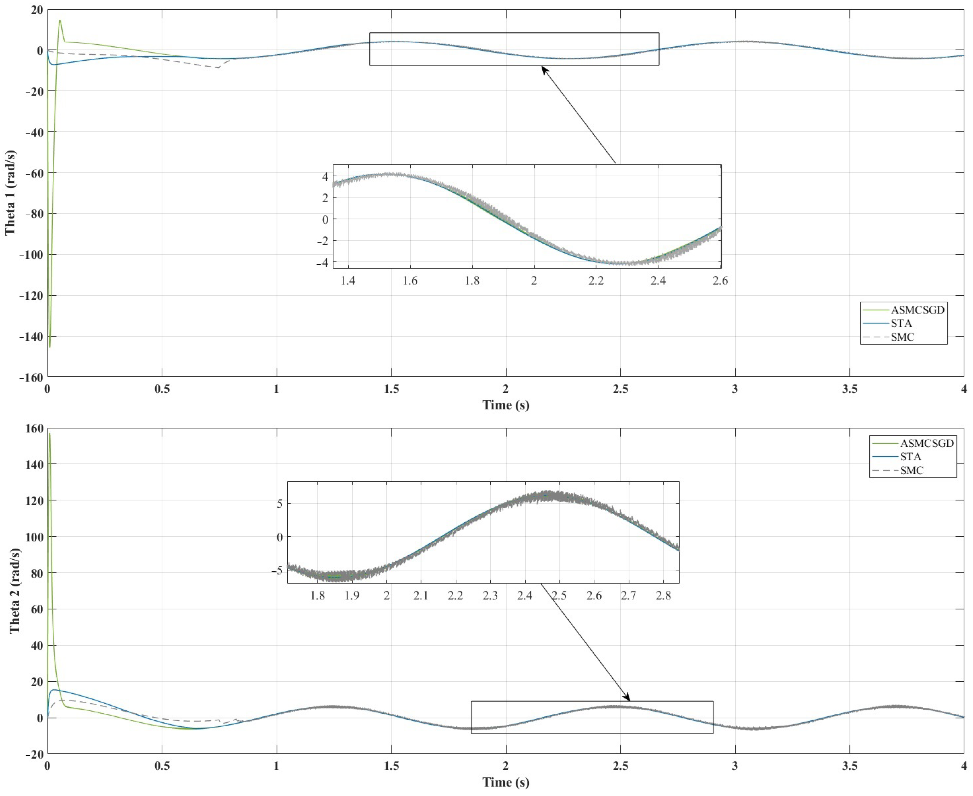
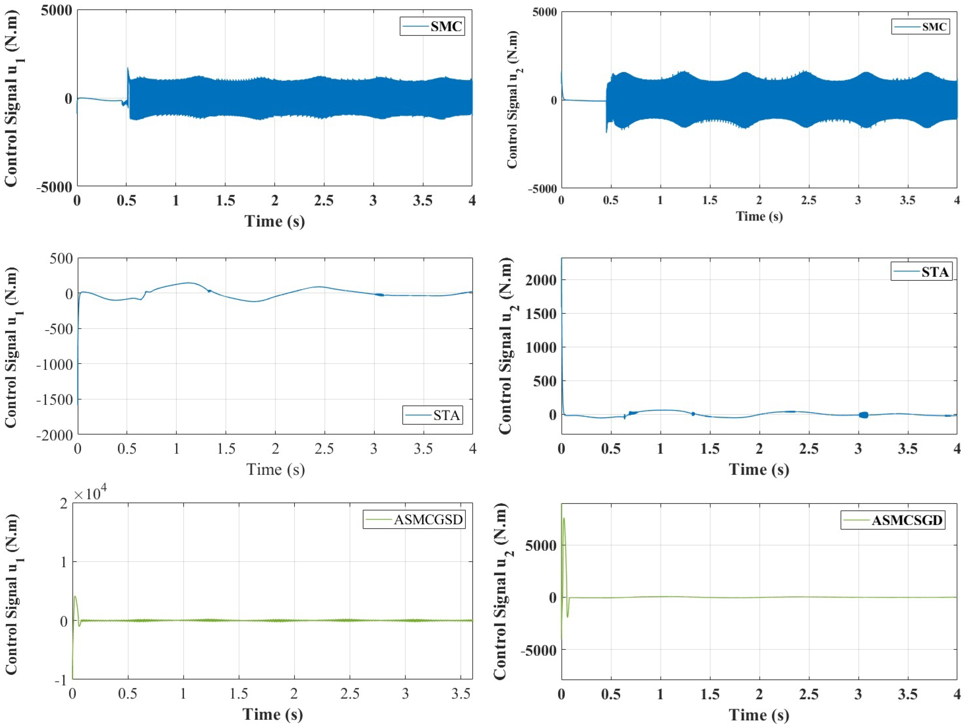
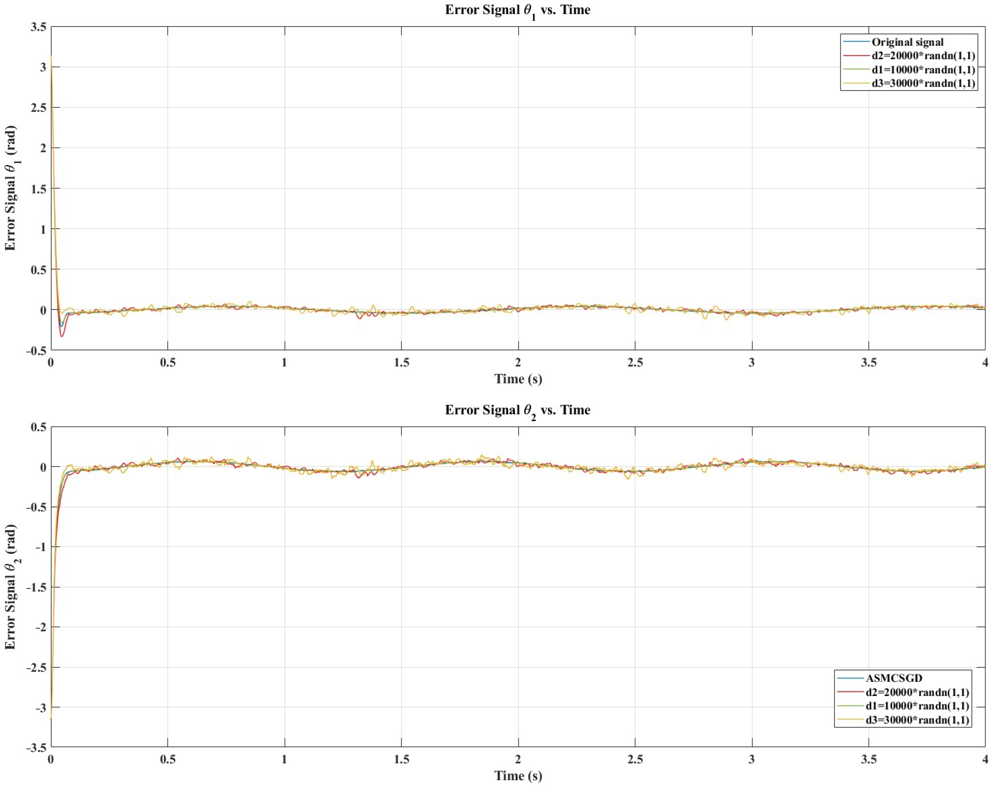
5. Results and Discussion

Table 1. Controllers upper and lower bounds.

Control Strategy		${\mathit{K}}_{\mathit{p}}$	${\mathit{K}}_{\mathit{d}}$	${\mathit{k}}_{\mathit{s}}$	${\mathit{\lambda }}_{\mathbf{1}}$	${\mathit{\lambda }}_{\mathbf{2}}$	$\mathit{\mu }$
ASMCSGD	Min	0	0	-	-	1	0
	Max	8000	200	-	-	2	1
STA	Min	0	0	0	0	-	-
	Max	8000	60	200	200	-	-
SMC	Min	0	0	-	-	-	-
	Max	8000	60	-	-	-	-

presents the upper and lower bounds for the parameters of the typical ASMCSGD, STA, and SMC controllers. The GWO is employed to tune and optimize the coefficients of the proposed controller $[K_p,K_d,K_s,{\lambda }_1,{\lambda }_2,\mu ]$ by minimizing the objective functions. The optimization process uses a population size of 20 wolves and is run for a maximum of 100 iterations. Both the population size and the number of iterations were chosen based on the trial-and-error method, balancing computational efficiency and optimization performance [48]. The objective function is defined based on the motion trajectory error of the joints and is outlined as follows [18]:

$$O=\sqrt{{\int }_0^{\infty }{\left|e_1\left(t\right)\right|}^{2}dt}+\sqrt{{\int }_0^{\infty }{\left|e_2\left(t\right)\right|}^{2}dt}$$

(44)

where $e_1\left(t\right)=q_1\left(t\right)-q_{d1}\left(t\right)$ and $e_2\left(t\right)=q_2\left(t\right)-q_{d2}\left(t\right)$.

The specified motion trajectories are given as follows:

$$\begin{array}{cc}\hfill {\theta }_{d1}\left(t\right)& =sin\left(4.17t\right)\hfill \\ \hfill {\theta }_{d2}\left(t\right)& =1.2sin\left(5.11t\right)\hfill \end{array}$$

where the initial values for the system are set as follows:

$$q_1\left(0\right)=\pi ,q_2\left(0\right)=-\pi ,{\dot{q}}_1\left(0\right)=0\mathrm{and}{\dot{q}}_2\left(0\right)=0$$

After optimizing the ASMCSGD, STA, and SMC controllers using GWO, the resulting controller parameters are listed in

Table 2. Controllers obtained gains.

Controller	${\mathit{K}}_{\mathit{p}}$	${\mathit{K}}_{\mathit{d}}$	${\mathit{k}}_{\mathit{s}}$	${\mathit{\lambda }}_{\mathbf{1}}$	${\mathit{\lambda }}_{\mathbf{2}}$	$\mathit{\mu }$
ASMCSGD	8000	100	-	-	-	$0.0101$
STA	8000	$49.4$	-	10	$7.8$	-
SMC	2078	$53.2$	200	-	-	-

.

Table 3. The RMSE for different control strategies.

Controller	RMSE for ${\mathit{\theta }}_{\mathbf{1}}$	RMSE for ${\mathit{\theta }}_2$
ASMCSGD	$0.12758$	$0.13387$
STA	$0.1813$	$0.1953$
SMC	$0.24505$	$0.29112$

shows that the tracking performance of the robotic arm improves slightly with the ASMCSGD compared with the conventional controllers across the desired trajectories. Specifically, ASMCSGD exhibits notably lower trajectory errors and a smaller root mean square error (RMSE) compared with other controllers. As it can be observed in Table 3, the ASMCSGD controller achieves an RMSE of $0.12758$ for ${\theta }_1$ and $0.13387$ for ${\theta }_2$. The STA controller shows RMSE values of $0.1813$ for ${\theta }_1$ and $0.1953$ for ${\theta }_2$, while the SMC controller records the highest RMSE values of $0.24505$ for ${\theta }_1$ and $0.29112$ for ${\theta }_2$, indicating reduced tracking accuracy. These results highlight the superior performance of the ASMCSGD in trajectory tracking for robotic arms. The performance assessment is based on the RMSE, calculated using the following formula [49]:

$$RMSE=\sqrt{{\displaystyle \frac{1}{n}}\sum _{i=1}^n{\left(X\left(i\right)-X_r\left(i\right)\right)}^2}$$

(45)

where $X\left(i\right)$ and $X_r\left(i\right)$ represent the actual and reference values at the i-th data point, respectively, and n denotes the total number of data points.

Figure 5 illustrates the convergence rate of the ASMCSGD-GWO across iterations, demonstrating efficient convergence and stability within a reasonable number of iterations. This underscores the robustness and effectiveness of the optimization process in determining the optimal control parameters for the controllers.

Figure 6 illustrates the position tracking control of $q_1$ and $q_2$ using ASMCSGD, STA, and SMC. It is evident from the figure that ASMCSGD achieves a quicker and more efficient alignment with the reference trajectory, with a response time of 0.056 s for ${\theta }_1$ and 0.77 s for ${\theta }_2$, compared with the STA method, which has response times of 0.55 s for ${\theta }_1$ and 0.52 s for ${\theta }_2$, and the SMC method, which has response times of $0.81s$ for ${\theta }_1$ and $0.66s$ for ${\theta }_2$. This demonstrates the superior performance of the ASMCSGD controller in achieving faster trajectory tracking. The 2-DoF robot manipulator, when controlled by ASMCSGD, reaches the desired trajectory more swiftly and accurately than with the other controllers, though STA and SMC also demonstrate satisfactory responses and good performance. Figure 7 depicts the position tracking error of $q_1$ and $q_2$ under ASMCSGD, STA, and SMC. As shown in Figure 7, ASMCSGD results in the smallest tracking error, followed by STA and then SMC. The velocity of joints 1 and 2 is shown in Figure 8 under applied controllers. According to Figure 8, the fastest controller is ASMCSGD, which makes the 2-DoF robot manipulator settle immediately to the set point in comparison to the other STA and SMC. In addition, the ASMCSGD and STA controllers exhibit minimal chattering, with velocity fluctuations nearly vanishing. This contrasts with the SMC controllers, where noticeable chattering is present. Specifically, the chattering amplitude for STA is observed at some points, while for ASMCSGD, it is almost negligible. Figure 9 illustrates the control output signals for the ASMCSGD, STA, and SMC controllers, highlighting noticeable differences in their performance. The SMC controller shows significant oscillations in its control signal, starting around $0.5$ seconds and continuing for the rest of the simulation. These oscillations indicate less stable control performance, which could lead to undesirable effects in real-world applications. The STA controller, while more stable than the SMC, still experiences occasional oscillations in the control signal. These brief instabilities, though less severe than those in the SMC, suggest potential moments of instability. This smoothness highlights the controller’s stability and precision, reinforcing its superiority. The ASMCSGD’s ability to maintain a consistent control signal without oscillations reflects its enhanced robustness and effectiveness in handling high-precision tasks, as also evidenced by the RMSE values and reduced velocity chattering in the results. In addition, random noise was applied to test the robustness of the proposed control method, as depicted in Figure 10. Various levels of noise were tested, ranging from $1\times \mathrm{randn}(1,1)$ to 10,000 × randn(1,1). Notably, noise levels from $1\times \mathrm{randn}(1,1)$ to 10,000 × randn(1,1) had minimal impact on the error signal, which remained largely unaffected. However, when the noise was increased beyond 10,000 × randn(1,1), the error signal began to exhibit significant interference, revealing the controller’s sensitivity to higher disturbance levels. This highlights the importance of robustness to noise in practical applications of the ASMCSGD scheme, where effectively managing such disturbances is crucial for maintaining accurate trajectory tracking and overall performance in dynamic environments. Introducing noise in the testing phase is crucial as it simulates real-world conditions, allowing for the assessment of the controller’s robustness, reliability, and ability to reduce chattering and maintain stability under unexpected disturbances.

6. Conclusions

This study presents a novel adaptive sliding mode control with stochastic gradient descent (ASMCSGD) approach for 2-DoF robot arm manipulators, demonstrating superior robustness, reduced chattering, and precise trajectory tracking compared with conventional SMC and STA controllers. The ASMCSGD controller achieves small root mean squared errors (RMSE) of $0.12758$ for ${\theta }_1$ and $0.13387$ for ${\theta }_2$, outperforming the SMC controller with RMSE values of $0.24505$ for ${\theta }_1$ and $0.29112$ for ${\theta }_2$ and the STA controller with RMSE values of $0.1813$ for ${\theta }_1$ and $0.1953$ for ${\theta }_2$. The ASMCSGD controller effectively manages varying disturbances and noise levels, maintaining robust performance in challenging conditions. This research underscores the ASMCSGD controller’s effectiveness in enhancing trajectory tracking and reducing chattering, making it a promising approach for robust control in various robotic applications.

In addition, the use of SGD for parameter adaptation in the ASMCSGD controller provides significant advantages over other optimization techniques, such as nature-inspired optimization algorithms. The SGD offers faster convergence and is highly effective in handling uncertainties and noisy environments. This efficiency is crucial for real-time applications, where rapid and reliable parameter updates are essential. Compared with nature-inspired optimization algorithms, which can be computationally intensive and slower to converge, SGD’s quick adaptability makes it particularly well-suited for dynamic and uncertain conditions. This practical advantage further enhances the ASMCSGD controller’s appeal for industrial automation and real-world robotic applications.

Furthermore, the ASMCSGD controller offers significant practical implications for the industry, particularly in terms of cost, scalability, and ease of integration. Its software-based architecture can be integrated into existing hardware setups without requiring expensive modifications, offering a cost-effective solution for industrial automation. The controller’s ability to adapt to a wide range of dynamic systems makes it highly scalable and suitable for various sectors, such as manufacturing, robotics, and autonomous systems. These features highlight the commercial potential and long-term impact of the proposed solution, demonstrating its viability for real-world applications.

References

1. Lamon, E.; Leonori, M.; Kim, W.; Ajoudani, A. Towards an intelligent collaborative robotic system for mixed case palletizing. In Proceedings of the 2020 IEEE International Conference on Robotics and Automation (ICRA), Paris, France, 31 May 2020–31 August 2020; pp. 9128–9134. [Google Scholar]
2. Sathish Kumar, A.; Naveen, S.; Vijayakumar, R.; Suresh, V.; Asary, A.R.; Madhu, S.; Palani, K. An intelligent fuzzy-particle swarm optimization supervisory-based control of robot manipulator for industrial welding applications. Sci. Rep. 2023, 13, 8253. [Google Scholar] [CrossRef] [PubMed]
3. Shanmugasundar, G.; Sapkota, G.; Čep, R.; Kalita, K. Application of MEREC in multi-criteria selection of optimal spray-painting robot. Processes 2022, 10, 1172. [Google Scholar] [CrossRef]
4. Bottin, M.; Cocuzza, S.; Massaro, M. Variable stiffness mechanism for the reduction of cutting forces in robotic deburring. Appl. Sci. 2021, 11, 2883. [Google Scholar] [CrossRef]
5. Blatnický, M.; Dižo, J.; Gerlici, J.; Sága, M.; Lack, T.; Kuba, E. Design of a robotic manipulator for handling products of automotive industry. Int. J. Adv. Robot. Syst. 2020, 17, 1729881420906290. [Google Scholar] [CrossRef]
6. Li, R.; Qiao, H. A survey of methods and strategies for high-precision robotic grasping and assembly tasks—Some new trend. IEEE/ASME Trans. Mechatron. 2019, 24, 2718–2732. [Google Scholar] [CrossRef]
7. Spong, M.W.; Hutchinson, S.; Vidyasagar, M. Robot modeling and control. IEEE/ASME Trans. Mechatron. 2019, 24, 2718–2732. [Google Scholar]
8. Ghosh, A.; Krishnan, T.R.; Tejaswy, P.; Mandal, A.; Pradhan, J.K.; Ranasingh, S. Design and implementation of a 2-DoF PID compensation for magnetic levitation systems. ISA Trans. 2014, 53, 1216–1222. [Google Scholar] [CrossRef]
9. Bi, M. Control of robot arm motion using trapezoid fuzzy two-degree-of-freedom PID algorithm. Symmetry 2020, 12, 665. [Google Scholar] [CrossRef]
10. Zhao, X.; Lin, Z.; Fu, B.; He, L.; Fang, N. Research on automatic generation control with wind power participation based on predictive optimal 2-degree-of-freedom PID strategy for multi-area interconnected power system. Energies 2018, 11, 3325. [Google Scholar] [CrossRef]
11. Efe, M.Ö. Fractional fuzzy adaptive sliding-mode control of a 2-DoF direct-drive robot arm. IEEE Trans. Syst. Man Cybern. Part Cybern. 2018, 38, 1561–1570. [Google Scholar] [CrossRef]
12. Tuan, H.M.; Sanfilippo, F.; Hao, N.V. A novel adaptive sliding mode controller for a 2-DoF elastic robotic arm. Robotics 2022, 11, 47. [Google Scholar] [CrossRef]
13. Patel, K.; Mehta, A. Discrete-time event-triggered higher order sliding mode control for consensus of 2-DoF robotic arms. Eur. J. Control 2020, 56, 231–241. [Google Scholar] [CrossRef]
14. El-Khatib, M.F.; Maged, S.A. Low level position control for 4-DoF arm robot using fuzzy logic controller and 2-DoF PID controller. In Proceedings of the 2021 International Mobile, Intelligent, and Ubiquitous Computing Conference (MIUCC), Cairo, Egypt, 26–27 May 2021; pp. 258–262. [Google Scholar]
15. Bikova, M.; Latkoska, V.O.; Hristov, B.; Stavrov, D. Path planning using fuzzy logic control of a 2-DoF robotic arm. In Proceedings of the 2022 IEEE 17th International Conference on Control & Automation (ICCA), Naples, Italy, 27–30 June 2022; pp. 998–1003. [Google Scholar]
16. Mohammed, A.A.; El-Nagar, A.M.; Elsheikh, E.A.; El-Bardini, M. Embedded adaptive 2-DoF PID controller for robot manipulator using a supervisory fuzzy logic system. Menoufia J. Electron. Eng. Res. 2022, 31, 55–62. [Google Scholar] [CrossRef]
17. Al-Darraji, I.; Piromalis, D.; Kakei, A.A.; Khan, F.Q.; Stojmenovic, M.; Tsaramirsis, G.; Papageorgas, P.G. Adaptive robust controller design-based RBF neural network for aerial robot arm model. Electronics 2021, 10, 831. [Google Scholar] [CrossRef]
18. Rahmani, M.; Komijani, H.; Rahman, M.H. New sliding mode control of 2-DoF robot manipulator based on extended grey wolf optimizer. Int. J. Control. Autom. Syst. 2020, 18, 1572–1580. [Google Scholar] [CrossRef]
19. Ren, B.; Wang, Y.; Chen, J. Trajectory-tracking-based adaptive neural network sliding mode controller for robot manipulators. J. Comput. Inf. Sci. Eng. 2020, 20, 031009. [Google Scholar] [CrossRef]
20. Thi, H.L.; Dang, V.T.; Nguyen, N.T.; Le, D.T.; Nguyen, T.L. A neural network-based fast terminal sliding mode controller for dual-arm robots. In International Conference on Engineering Research and Applications; Springer: Cham, Switzerland, 2022; pp. 42–52. [Google Scholar]
21. Cai, B.; Zhang, Y. Different-level redundancy-resolution and its equivalent relationship analysis for robot manipulators using gradient-descent and Zhang’s neural-dynamic methods. IEEE Trans. Ind. Electron. 2011, 59, 3146–3155. [Google Scholar] [CrossRef]
22. Youns, M.D.; Attya, S.M.; Abdulla, A.I. Position control of robot arm using genetic algorithm based PID controller. Al-Rafidain Eng. Mosul Iraq 2013, 21, 19–30. [Google Scholar]
23. Bingol, M.C.; Akpolat, Z.H.; Koca, G.O. Robust control of a robot arm using an optimized PID controller. In Mechatronics 2017: Recent Technological and Scientific Advances; Springer: Berlin/Heidelberg, Germany, 2018; pp. 484–492. [Google Scholar]
24. Zhao, J.; Han, L.; Wang, L.; Yu, Z. The fuzzy PID control optimized by genetic algorithm for trajectory tracking of robot arm. In Proceedings of the 2016 12th World Congress on Intelligent Control and Automation (WCICA), Guilin, China, 12–15 June 2016; pp. 556–559. [Google Scholar]
25. Pan, Y.; Li, X.; Wang, H.; Yu, H. Continuous sliding mode control of compliant robot arms: A singularly perturbed approach. Mechatronics 2018, 52, 127–134. [Google Scholar] [CrossRef]
26. Zakia, U.; Moallem, M.; Menon, C. PID-SMC controller for a 2-DoF planar robot. In Proceedings of the 2019 International Conference on Electrical, Computer and Communication Engineering (ECCE), Cox’s Bazar, Bangladesh, 7–9 February 2019; pp. 1–5. [Google Scholar]
27. Eltayeb, A.; Rahmat, M.F.; Eltoum, M.M.; MH, S.I.; Basri, M.A.M. Adaptive sliding mode control design for the 2-DoF robot arm manipulators. In Proceedings of the 2019 International Conference on Computer, Control, Electrical, and Electronics Engineering (ICCCEEE), Khartoum, Sudan, 21–23 September 2019; pp. 1–5. [Google Scholar]
28. Zhang, J.; Yu, L.; Tang, J.; Ding, L. Dual Surface Sliding Mode Controller of Torque Tracking for 2-DoF Robotic Arm Driven by Electrohydraulic Servo System. Eng. Lett. 2018, 26. [Google Scholar]
29. Jouila, A.; Nouri, K. An adaptive robust nonsingular fast terminal sliding mode controller based on wavelet neural network for a 2-DoF robotic arm. J. Frankl. Inst. 2020, 357, 13259–13282. [Google Scholar] [CrossRef]
30. Mohan, V.; Chhabra, H.; Rani, A.; Singh, V. An expert 2DOF fractional order fuzzy PID controller for nonlinear systems. Neural Comput. Appl. 2019, 31, 4253–4270. [Google Scholar] [CrossRef]
31. Howard, I.S.; Ingram, J.N.; Wolpert, D.M. A modular planar robotic manipulandum with end-point torque control. J. Neurosci. Methods 2009, 181, 199–211. [Google Scholar] [CrossRef] [PubMed]
32. Sachan, S.; Swarnkar, P. Intelligent fractional order sliding mode based control for surgical robot manipulator. Electronics 2023, 12, 729. [Google Scholar] [CrossRef]
33. Song, Z.; Bao, D.; Wang, W.; Zhao, W. Adaptive Dynamic Boundary Sliding Mode Control for Robotic Manipulators under Varying Disturbances. Electronics 2024, 13, 900. [Google Scholar] [CrossRef]
34. Sinha, S.; Nethi, A.; Jetta, M. Multiplicative Gaussian Noise Removal using Partial Differential Equations and Activation Functions: A Robust and Stable Approach. In Proceedings of the 7th International Conference on Algorithms, Computing and Systems, Larissa, Greece, 19–21 October 2023; pp. 161–170. [Google Scholar]
35. Guo, K.; Shi, P.; Wang, P.; He, C.; Zhang, H. Non-singular terminal sliding mode controller with nonlinear disturbance observer for robotic manipulator. Electronics 2023, 12, 849. [Google Scholar] [CrossRef]
36. Song, Y.; Liu, Z.; Ouyang, H.; Wang, H.; Lu, X. Sliding Mode Control with PD Sliding Surface for High-Speed Railway Pantograph-Catenary Contact Force under Strong Stochastic Wind Field. Pshock Vib. 2017, 2017, 4895321. [Google Scholar] [CrossRef]
37. Dang, S.T.; Dinh, X.M.; Kim, T.D.; Xuan, H.L.; Ha, M.H. Adaptive backstepping hierarchical sliding mode control for 3-wheeled mobile robots based on RBF neural networks. Electronics 2023, 12, 2345. [Google Scholar] [CrossRef]
38. Zhao, M.; Qian, H.; Zhang, Y. Predefined-Time Adaptive Fast Terminal Sliding Mode Control of Aerial Manipulation Based on a Nonlinear Disturbance Observer. Electronics 2024, 13, 2746. [Google Scholar] [CrossRef]
39. Levant, A. Sliding order and sliding accuracy in sliding mode control. Int. J. Control 1993, 58, 1247–1263. [Google Scholar] [CrossRef]
40. Sehab, R.; Akrad, A.; Saadi, Y. Super-twisting sliding mode control to improve performances and robustness of a switched reluctance machine for an electric vehicle drivetrain application. Energies 2023, 16, 3212. [Google Scholar] [CrossRef]
41. Moreno, J.A.; Osorio, M. Strict Lyapunov functions for the super-twisting algorithm. IEEE Trans. Autom. Control 2012, 57, 1035–1040. [Google Scholar] [CrossRef]
42. Rahmani, M. Control of a caterpillar robot manipulator using hybrid control. Microsyst. Technol. 2019, 25, 2841–2854. [Google Scholar] [CrossRef]
43. Silaa, M.Y.; Bencherif, A.; Barambones, O. A novel robust adaptive sliding mode control using stochastic gradient descent for PEMFC power system. Int. J. Hydrogen Energy 2023, 48, 17277–17292. [Google Scholar] [CrossRef]
44. Silaa, M.Y.; Barambones, O.; Bencherif, A. A novel adaptive PID controller design for a PEM fuel cell using stochastic gradient descent with momentum enhanced by whale optimizer. Electronics 2022, 11, 2610. [Google Scholar] [CrossRef]
45. Mirjalili, S.; Mirjalili, S.M.; Lewis, A. Grey wolf optimizer. Adv. Eng. Softw. 2014, 69, 46–61. [Google Scholar] [CrossRef]
46. Silaa, M.Y.; Barambones, O.; Derbeli, M.; Napole, C.; Bencherif, A. Fractional order PID design for a proton exchange membrane fuel cell system using an extended grey wolf optimizer. Processes 2022, 10, 450. [Google Scholar] [CrossRef]
47. Silaa, M.Y.; Barambones, O.; Bencherif, A.; Rahmani, A. A New MPPT-Based Extended Grey Wolf Optimizer for Stand-Alone PV System: A Performance Evaluation versus Four Smart MPPT Techniques in Diverse Scenarios. Inventions 2023, 8, 142. [Google Scholar] [CrossRef]
48. Rao, S.S. Engineering Optimization: Theory and Practice; John Wiley & Sons: Hoboken, NJ, USA, 2019. [Google Scholar]
49. Silaa, M.Y.; Bencherif, A.; Barambones, O. Indirect Adaptive Control Using Neural Network and Discrete Extended Kalman Filter for Wheeled Mobile Robot. Actuators 2024, 13, 51. [Google Scholar] [CrossRef]
Figure 1. The 2 DoF rigid-link robot manipulator.
Electronics 13 03903 g001
Figure 2. Block diagram of the proposed control method.
Electronics 13 03903 g002
Figure 3. The SGD technique.
Electronics 13 03903 g003
Figure 4. The GWO flowchart [46].
Electronics 13 03903 g004
Figure 5. The convergence rate for ASMCSGD-GWO under iterations.
Electronics 13 03903 g005
Figure 6. Position tracking joints under ASMCSGD, STA, and SMC controllers.
Electronics 13 03903 g006
Figure 7. Position tracking error joints under ASMCSGD, STA, and SMC controllers.
Electronics 13 03903 g007
Figure 8. Velocity joints under ASMCSGD, STA, and SMC controllers.
Electronics 13 03903 g008
Figure 9. Control signals for the under ASMCSGD, STA, and SMC controllers.
Electronics 13 03903 g009
Figure 10. Position tracking error of joints of the proposed controller under random noises application.
Electronics 13 03903 g010