Diffusion Model for Camouflaged Object Segmentation with Frequency Domain

Abstract

The task of camouflaged object segmentation (COS) is a challenging endeavor that entails the identification of objects that closely blend in with their surrounding background. Furthermore, the camouflaged object’s obscure form and its subtle differentiation from the background present significant challenges during the feature extraction phase of the network. In order to extract more comprehensive information, thereby improving the accuracy of COS, we propose a diffusion model for a COS network that utilizes frequency domain information as auxiliary input, and we name it FreDiff. Firstly, we proposed a frequency auxiliary module (FAM) to extract frequency domain features. Then, we designed a Global Fusion Module (GFM) to make FreDiff pay attention to the global features. Finally, we proposed an Upsample Enhancement Module (UEM) to enhance the detailed information of the features and perform upsampling before inputting them into the diffusion model. Additionally, taking into account the specific characteristics of COS, we develop the specialized training strategy for FreDiff. We compared FreDiff with 17 COS models on the four challenging COS datasets. Experimental results showed that FreDiff outperforms or is consistent with other state-of-the-art methods under five evaluation metrics.

1. Introduction

Camouflage involves an object altering its color, texture, shape, and behavior to reduce the likelihood of detection, thus achieving self-protection or misleading the enemy in both natural and artificial environments. In nature, many animals possess exceptional camouflage abilities, mimicking the colors or textures of their surroundings to conceal themselves [1]. For example, antelopes utilize their spiral-shaped horns, which resemble the vines of shrubs, to evade predators and approach prey. In the military domain, camouflaging objects plays a crucial role, with military facilities, equipment, and personnel often requiring camouflage to blend into their surroundings, thus decreasing the likelihood of being detected by the enemy [2]. The task of camouflaged object segmentation (COS) aims to segment camouflaged objects from complex scenes where they are highly integrated with the environment. COS finds extensive downstream applications, such as in medical segmentation [3], industrial quality inspection [4], agricultural pest detection [5], and remote sensing [6].

In recent years, with the development of deep learning, researchers have pushed the performance of COS algorithms to new heights. For instance, most existing COS models adopt a multi-stage learning approach [7,8,9,10], where they first make a coarse prediction of the overall region and then refine the preliminary results obtained from the previous stage using various methods to arrive at the final prediction. It is also feasible to combine auxiliary tasks with the COS task. Similar to COS, Salient Object Segmentation (SOS) [11] requires extracting object attributes, but one focuses on extracting salient objects while the other focuses on extracting camouflaged objects. Although COS and SOS differ in terms of the distinguishability between the target and the background as well as their application scenarios, the similarities and complementarities between SOS and COS can be leveraged to enhance each other’s performance. Li et al. proposed UJSC [12], which combines SOS and COS tasks by treating simple samples from the camouflaged dataset as difficult samples in the SOS task, utilizing the contradictory information between them to enhance their respective segmentation capabilities. CamDiff employs a diffusion model to synthesize salient objects in camouflaged images, thereby increasing image diversity and improving the model’s robustness and segmentation performance [13]. Some studies attempt to utilize depth information [14] and boundary information [15] to reduce background interference and determine object contours, thereby guiding the model to precisely locate camouflaged objects.

Most COS methods are primarily built upon general semantic segmentation, employing a single network to specifically extract object features and subsequently utilizing a decoder to directly obtain the predicted segmentation mask. However, this paradigm tends to overlook global information and confuse the subtle boundary features between camouflaged objects and their environments, resulting in unsatisfactory segmentation predictions. Furthermore, these methods heavily rely on pre-annotated ground truth (GT) masks, which may lead to the model becoming overly sensitive and dependent on detailed features, thereby causing a high false alarm rate in segmentation. In recent years, guided diffusion models have developed rapidly, which guide the generation process of diffusion models by adding auxiliary information such as text, physics, boundaries, and other conditions [16,17,18].

Addressing the aforementioned challenges, we propose a frequency-guided camouflaged object segmentation network based on a diffusion model, termed FreDiff. Specifically, this approach leverages the frequency information of images to extract more comprehensive details, thereby tackling the issue where similar features are easily confounded in existing frameworks. By leveraging a diffusion model, the task of image segmentation is transformed into an image generation task. Through continuous iterative refinement and denoising of the prediction maps, the high false alarm rate problem inherent in COS models is alleviated. Figure 1 elucidates the distinctions between the COS network grounded on the diffusion model and conventional COS networks.

Specifically, we design the frequency auxiliary module (FAM) and simultaneously input the image into both the object segmentation network and the frequency feature extraction module. Subsequently, we design the Global Fusion Module (GFM) to focus on global information during feature extraction, thereby enhancing the understanding of object relationships within the images. Furthermore, we propose the Upsample Enhancement Module (UEM) that focuses on detailed information such as object boundaries and textures, aiming to reduce the probability of missed detections. Lastly, we optimize the noise schedule of the diffusion model specifically for the characteristics of the COS task, improving the overall segmentation performance of the model by accelerating the noise injection process during training. To summarize, the main contributions of this paper are as follows:

• We construct a diffusion model for the COS network with the frequency domain, FreDiff. We propose FAM to extract frequency domain information from images and achieve feature alignment through the feature fusion module, thereby obtaining more comprehensive information about camouflaged objects.
• We design GFM and UEM, which allow FreDiff to focus on global features and boundary detail features, respectively, thereby enhancing its understanding of image information and refining edge details.
• We propose a noise schedule for the diffusion model tailored for COS, which improves the model’s segmentation performance and training efficiency by increasing the speed of noise addition during the training stage.

The rest of this paper is structured as follows: In Section 2, we introduce the related work. Section 3 describes the network structure of FreDiff in detail, as well as its mathematical derivation process, training, and inference strategies. Section 4 gives the discussions of experimental results. Finally, we summarize the research content in Section 5.

2. Related Work

2.1. Camouflaged Object Segementation

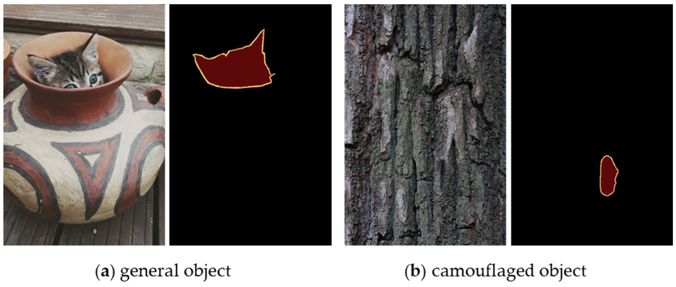
COS is a task aimed at mimicking the visual system of predators to segment objects hidden in the environment. Compared with other segmentation tasks, COS is a category-agnostic task, where a camouflaged object refers to all pixel points in the camouflaged area of an image. This task involves predicting the probability of each pixel in an image under the supervision of a binary mask, requiring the COS algorithm to assign labels to each pixel point. A label value of 0 indicates that the pixel does not belong to a camouflaged object, while a label value of 1 indicates that the pixel fully belongs to a camouflaged object [19]. This is used to determine whether each pixel belongs to a camouflaged object. Figure 2 shows the difference between camouflaged objects and ordinary objects, with camouflaged objects being more difficult to recognize compared to ordinary objects.

In recent years, with the rapid development of deep learning technology, the demand for recognizing camouflaged objects has increased significantly, leading to growing attention on the task of COS. In 2019, Le et al. proposed the Anabranch Network (ANet) architecture as a basic framework for COS [20]. In 2020, Fan et al. introduced the COS task and developed a simple yet effective Search Identification Network (SINet) [1]. In 2021, Lv et al. proposed the first ranking-based network, Rank-Net, for simultaneously locating, segmenting, and identifying camouflaged objects, and released the NC4K dataset [21]. In 2022, Zhang et al. proposed the first camouflaged object segmentation network that introduces depth prior information, which can reduce the ambiguity of RGB features in complex scenes and mitigate camouflage effects, making it more sensitive to capturing the true boundaries of camouflaged objects [22]. In 2023, He et al. proposed the first end-to-end weakly supervised COS framework and released the first dataset with scribble annotations for weakly supervised COS [23]. In 2024, Pang et al. proposed ZoomNext, which introduces a unified collaborative pyramid network that mimics the zoom-in and zoom-out behavior of human observers when viewing blurred images and videos [24]. Through continuous development, COS has become an important task in the field of computer vision, spawning novel and diverse research ideas that enhance the ability to extract features of camouflaged objects.

2.2. Diffusion Model

The diffusion model, originating from non-equilibrium thermodynamic theory, is a probabilistic generative model. The core idea of the diffusion model is to generate high-quality data by gradually adding noise to the data and learning to reverse this process. The working principle of the diffusion model is divided into two main stages: the forward diffusion process and the reverse diffusion process. In the forward diffusion process, the model gradually adds Gaussian noise to the data, forming a Markov chain, until the data in the image are completely covered by noise. In the reverse diffusion process, a neural network is trained to learn how to gradually denoise from noisy data and recover the original data. The diffusion model has received widespread attention for its powerful generative capabilities and ability to retain details, enabling it to demonstrate outstanding performance in various fields such as image generation, image restoration, audio generation, and style transfer. Since the introduction of the denoising diffusion probabilistic model (DDPM) in 2020 by Ho et al. [25], DDPM was the first application of the denoising diffusion probabilistic model to image generation tasks, which laid the foundation for the use of diffusion models in the field of image generation. In 2022, Wu et al. proposed MedSegDiff, the first network based on the diffusion probabilistic model (DPM) for general medical image segmentation tasks [26]. In 2023, Chen et al. introduced a diffusion model for COS named Camodiffusion, which provides a new perspective and solves many existing problems in COS tasks [27]. In the same year, by modeling the object detection task as a denoising diffusion process from noise boxes to object boxes, DiffusionDet successfully introduced the advantages of generative models into object detection [28].

2.3. Frequency-Guided Segmentation

Frequency representation, as a new paradigm for learning differences between categories, can uncover information overlooked by human vision. By utilizing more frequency information, the differences between categories can be enhanced, making the boundaries between each category clearer and thereby improving the effectiveness of semantic segmentation. In COS tasks, it is often necessary to retain and enhance the edge information of camouflaged objects, which is mostly located in the higher frequency range. Frequency information reveals the frequency distribution of the image, helping to determine the target information in the image.

In the past few years, frequency-aided techniques have been widely used in object segmentation tasks, but their application in COS-related tasks has been relatively limited. In 2020, Xu et al. proposed using the spatial frequency domain instead of RGB images as input to CNNs for extracting feature vectors [29]. This method can significantly reduce data transmission and improve model accuracy to some extent. In 2022, Zhong et al. proposed a method that utilizes frequency domain information to assist RGB information in the detection of camouflaged objects [30]. In 2023, Cong et al. adopted a two-stage model, including a frequency-guided coarse localization stage and a detail-preserving fine localization stage, to achieve the precise detection of camouflaged objects [31]. Also in 2023, Dong et al. proposed a headless lightweight semantic segmentation-specific architecture, AFFormer, which learns local descriptive representations of clustering prototypes from a frequency perspective [32]. This paper extracts frequency feature information and inputs it into a diffusion model to assist the model in generating high-quality segmentation results.

3. Methods

As illustrated in Figure 3, we propose a denoising diffusion probabilistic model for COS network FreDiff, which is an image generation model rooted in Markov chains. This process encompasses a forward training stage and a reverse sampling stage.

3.1. Mathematical Derivation

3.1.1. Forward Process

Given an initial data distribution, $z_0 ~ q(z)$, the forward diffusion process gradually adds random noise to the original input image $mas{k}_0$, where the noise follows a Gaussian distribution $\mathcal{N}(0,\mathsf{I})$. The image $mas{k}_t$ obtained at each step is only related to the noisy result $mas{k}_{t-1}$ of the previous step. This noising process continues for T steps, generating a series of noisy images, $mas{k}_1,mas{k}_2,\cdots mas{k}_T$, ultimately resulting in an image that tends to be pure noise.

In the process of adding noise to transform image data from $mas{k}_{t-1}$ to $mas{k}_t$, the variance of the noise is determined by a fixed value ${\beta }_T$ within the interval (0, 1), while the mean is determined by both this fixed value ${\beta }_T$ and the current image data $mas{k}_{t-1}$. The aforementioned noise addition process can be expressed mathematically as follows:

$$q(mas{k}_t|mas{k}_{t-1})=\mathcal{N}(mas{k}_t;\sqrt{1-{\beta }_t}mas{k}_{t-1},{\beta }_t\mathsf{I})$$

(1)

$$q(mas{k}_{1:T}|mas{k}_0)={\Pi }_{t=1}^{T}q(mas{k}_t|mas{k}_{t-1}),$$

(2)

where $t\in [1,T]$, $mas{k}_t$ represents the image at step t, and I represents a variance matrix that has the same dimensions as the input image.

It is not necessary to iteratively obtain $mas{k}_t$ from $mas{k}_0,mas{k}_1,\cdots$ step by step. Instead, the latent variable $mas{k}_t$ can be directly derived from $mas{k}_0$ and a fixed value sequence, ${\left\{{\beta }_T\in (0,1)\right\}}_{t=1}^T$. The formula is as follows:

$$q(mas{k}_t|mas{k}_0)=\mathcal{N}(mas{k}_t;\sqrt{{\overline{\alpha }}_t}mas{k}_0,(1-{\overline{\alpha }}_t)\mathsf{I})$$

(3)

In the formula, ${\alpha }_t:=1-{\beta }_t$ and ${\overline{\alpha }}_t:={\Pi }_{n=0}^t{\alpha }_n$.

3.1.2. Backward Process

The reverse process is a process of continuously removing noise, which reverses the direction of the aforementioned process. Given a noisy image $mas{k}_T$, it gradually denoises and restores it until the original image $mas{k}_0$ is finally recovered. Reversing the direction of the aforementioned process, we sample from $q(mas{k}_{t-1}|mas{k}_t)$ and reconstruct a real original sample within a random Gaussian distribution $\mathcal{N}(0,\mathsf{I})$, meaning that we obtain a real image from a completely chaotic noisy image. Therefore, it is necessary to learn a model, $p_{\theta }$, to approximate this conditional probability, so as to run the reverse diffusion process. The formula is as follows:

$$p_{\theta }(mas{k}_{0:T})=p(mas{k}_T){\Pi }_{t=1}^T{p}_{\theta }(mas{k}_{t-1}|mas{k}_t),$$

(4)

$$p_{\theta }(mas{k}_{t-1}|mas{k}_t)=N(mas{k}_{t-1};{\mu }_{\theta }(mas{k}_t,t),{\sum }_{\theta }(mas{k}_t,t)),$$

(5)

In the formula, the specific expressions of ${\mu }_{\theta }(mas{k}_t,t)$ and ${\sum }_{\theta }(mas{k}_t,t)$ can be represented by Formulas (6) and (7):

$${\mu }_{\theta }(mask,t)={\displaystyle \frac{1}{\sqrt{{\alpha }_t}}}(mas{k}_t-{\displaystyle \frac{{\beta }_t}{\sqrt{1-\overline{{\alpha }_t}}}}{\epsilon }_{\theta }(mas{k}_t,t)),$$

(6)

$${\sum }_{\theta }(mas{k}_t,t)=\widetilde{{\beta }_t}={\displaystyle \frac{(1-\overline{{\alpha }_{t-1}}){\beta }_t}{1-\overline{{\alpha }_t}}}\approx {\beta }_t.$$

(7)

where ${\mu }_{\theta }(mas{k}_t,t)$ denotes the mean, ${\sum }_{\theta }(mas{k}_t,t)$ denotes the variance, and $\theta$ represents the model parameters.

The reverse process can be summarized as follows: given $mas{k}_t$, first predict the Gaussian noise ${\epsilon }_{\theta }(mas{k}_t,t)$, then calculate the mean ${\mu }_{\theta }(mask,t)$ and variance ${\sum }_{\theta }(mas{k}_t,t)$ of $p_{\theta }(mas{k}_{t-1}|mas{k}_t)$, and finally iteratively derive $mas{k}_0$ through further steps.

3.2. FreDiff Architecture Design

The FreDiff we propose is depicted in Figure 4a. Firstly, the image is simultaneously input into the feature extraction backbone and FAM. Then, the extracted features are fused by FF and input into the GFM to make the model focus on global information. After that, it is input into the UEM to enhance the detail information. Next, the feature information and the mask image are input into the diffusion model together. Finally, the predicted mask is generated through iterative refinement.

3.2.1. Backbone

The backbone is capable of transforming data into more advanced and abstract feature representations, capturing important information within the data. Therefore, the backbone plays a crucial role in enhancing the performance of the entire model. This paper selects the PVTv2 backbone for experimentation [33]. The backbone structure is shown in Figure 4b. Specifically, given an input image of size $H\times W\times C$, it is divided into blocks of size $F\in {\mathbb{R}}^{{\displaystyle \frac{HW}{S^2}}}$. Convolution is applied with a stride of S, a kernel size of 2S − 1, and padding of S − 1. Then, the unfolded blocks are fed into a linear layer to obtain embedded blocks of scale $F\in {\mathbb{R}}^{{\displaystyle \frac{HW}{S^2}}\times C\prime }$. Finally, the embedded blocks, along with positional embedding information, are sent to the Transformer Encoder, whose output is reshaped to a size of $F\in {\mathbb{R}}^{{\displaystyle \frac{H}{S}}\times {\displaystyle \frac{W}{S}}\times C\prime }$. PVTv2 introduces a linear complexity attention layer named Linear Spatial Reduction Attention (Linear SRA), which significantly reduces the computational complexity of the model when processing high-resolution images. Variants such as B1, B2, etc., in PVTv2 represent different model versions of scales and configurations. They adapt to different computational resources and task requirements by adjusting hyperparameters. FreDiff selects PVTv2-B3 for the experiment.

3.2.2. FAM

Camouflaged objects are adept at utilizing colors and textures that are highly similar to their backgrounds to deceive the visual system. However, frequency information has the ability to uncover subtle differences between camouflaged objects and their backgrounds that are hard to detect in the spatial domain. For this purpose, we propose the frequency auxiliary module (FAM), which aims to extract frequency information from images and use it as auxiliary information for segmenting camouflaged objects.

The specific frequency auxiliary module is shown in Figure 5. Firstly, the input image is processed using the YCbCr color space, which can fully utilize its characteristics of separating luminance and chrominance, improve compression efficiency, and more accurately reflect the detailed features of the image while maintaining image quality. Then, the block processing and discrete cosine transform (DCT) are performed to obtain spectral information. The spectral information is integrated and output, which can be divided into high-frequency and low-frequency components. The high-frequency information $f_h$ enhances the detailed features such as edges and textures of the objects in the image, while the low-frequency information $f_{\mathrm{l}}$ forms the overall framework of the image. These two components are separately input into two multi-head self-attention modules, and their outputs are concatenated and reshaped to restore the original shape. Subsequently, multi-head self-attention is used to harmonize all frequency band information, and finally, frequency feature information $x_f$ is obtained through upsampling operations. The formulas for the progress are as follows:

$$f_h^{\prime }=\mathcal{M}(f_h)\oplus \mathit{up}(\mathcal{M}(f_{l\to h}),2),$$

(8)

$$f_l^{\prime }=\mathcal{M}(f_l)\oplus \mathit{down}(\mathcal{M}(f_{h\to l}),2),$$

(9)

$$x_f=\mathit{Re}(\mathcal{M}(\mathit{Re}(\mathit{Concat}(f_l^{\prime },f_h^{\prime })))),$$

(10)

where “up” represents the upsampling operation, “down” represents the downsampling operation, $\mathit{Re}$ represents the reshape operation, and $\mathcal{M}$ denotes processing by the multi-head self-attention mechanism.

To ensure the integrity of extracted features, we designed feature fusion (FF) to align frequency features with extraction from the backbone features, facilitating better integration into the network. Firstly, frequency features undergo frequency domain adjustment learning through an adaptive filter, which effectively eliminates noise components. Subsequently, features from the spatial and frequency domains are concatenated, and their common features are processed through a two-dimensional convolution with a kernel size of 3 and a sigmoid function to obtain $x_{\mathit{con}}$. The feature information from the two domains is separately merged with $x_{\mathit{con}}$, and finally, an addition operation is performed to obtain the ultimate fused features f. The formulas for the progress are as follows:

$$x_{\mathit{con}}=(\sigma (\mathit{Conv}(\mathit{Concat}(x_f,x\prime )))),$$

(11)

$$f=(x_{\mathit{con}}\otimes x_f)+(x_{\mathit{con}}\otimes x\prime ).$$

(12)

3.2.3. GFM

Global features can capture the overall shape, contour, and position distribution of the target in the image, helping the model to identify camouflaged objects holistically and reducing the misidentification of the background or other non-target objects as camouflaged objects, thereby improving the accuracy of segmentation. Therefore, we propose GFM, which performs feature enhancement learning in the spatial domain.

As shown in Figure 6, GFM captures further spatial information from shallow local detail features using 3 × 3 convolutions to obtain initial enhanced features. Next, multi-scale convolution processing is performed, generating richer and more comprehensive feature representations by convolving with different kernel sizes. Then, channel attention is obtained through one-dimensional convolution operations and the sigmoid function, and spatial information is aggregated by the global average pooling layer; this process reduces the number of parameters, thereby reducing overfitting. Finally, the channel attention is multiplied with the input features, and the channels are reduced by a 1 × 1 convolution layer to obtain the final output. This process can be expressed mathematically as

$$f_{conv3}={\mathcal{F}}_{conv3}(f)\oplus f,$$

(13)

$$f_{cat}=Concat({\mathcal{F}}_{conv3}(f_{conv3}),{\mathcal{F}}_{conv5}(f_{conv3}),{\mathcal{F}}_{conv7}(f_{conv3})),$$

(14)

$$f\prime ={\mathcal{F}}_{conv1}(GAP(\sigma ({\mathcal{F}}_{Conv1d}(f_{cat})))\otimes f_{cat}),$$

(15)

In the formula, GAP is the abbreviation for global average pooling, $\sigma$ represents the sigmoid activation function, $\otimes$ denotes element-wise multiplication, ${\mathcal{F}}_{\mathrm{convi}}$ represents i × i convolution, and ${\mathcal{F}}_{\mathrm{convld}}$ denotes the one-dimensional convolution operation and ⊕ denotes element-wise addition.

3.2.4. UEM

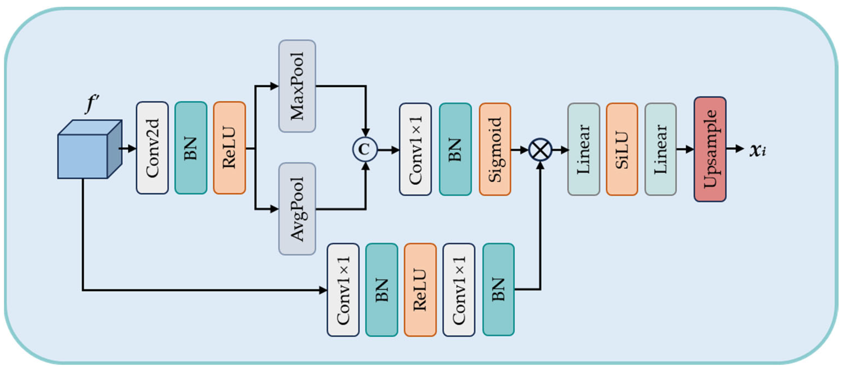
Feature enhancement can highlight the detail information in images, which is crucial for COS. We design the Upsample Enhancement Module (UEM), which can enhance the representation learning of feature details of camouflaged objects. Since some redundant information is introduced during feature extraction, UEM can make the model focus more on effective information such as the boundary feature and texture feature. The UEM structure is shown in Figure 7.

First, the feature f′ is input into a two-dimensional convolution layer, processed through a BN layer and ReLU function. Subsequently, the feature is fed into both an average pooling layer and a max pooling layer, and then we perform the concat operation. This approach effectively pays attention to the edge and texture details of the feature while preserving its background information. Finally, the fused feature is processed through a 1 × 1 convolution layer, a BN layer, and a sigmoid function to obtain f‴:

$$f″=\mathit{ReLU}(\mathit{BN}({\mathcal{F}}_{\mathit{conv}2d}(f\prime ))),$$

(16)

$$f‴=\sigma (\mathit{BN}({\mathcal{F}}_{\mathit{conv}1}(\mathit{Concat}(\mathit{AP}(f″),\mathit{MP}(f″)))),$$

(17)

where BN denotes Batch Normalization, ${\mathcal{F}}_{\mathrm{conv}2\mathrm{d}}$ represents two-dimensional convolution, $\mathit{ReLU}$ denotes the ReLU activate function, and AP and MP represent average pooling and maximum pooling, respectively. $\mathcal{L}\mathcal{N}$ denotes the Layer Norm and $\mathsf{\sigma }$ represents the sigmoid activate function.

Subsequently, the feature f′ is processed through a 1 × 1 convolution layer, a BN layer, and a ReLU function to obtain $f_i^{\prime }$. Then, the previously processed feature f‴ is fused with $f_i^{\prime }$, and the fused result is further processed through a linear operation and a SiLU activation function. Finally, the upsampling process is used to output the features as $x_i\in {\mathbb{R}}^{{\displaystyle \frac{H}{4}}\times {\displaystyle \frac{W}{4}}}$. This process can alternatively be represented mathematically as follows:

$$f_i^{\prime }=\mathit{BN}({\mathcal{F}}_{\mathit{conv}1}(\mathit{ReLU}(\mathit{BN}({\mathcal{F}}_{\mathit{conv}1}(f\prime ))))),$$

(18)

$$x_i=\mathit{Up}(\mathcal{L}(\mathit{SiLU}(\mathcal{L}(f‴\otimes f_i^{\prime })))),$$

(19)

In the formula, ${\mathcal{F}}_{\mathrm{convl}}$ represents 1 × 1 convolution, $\mathit{SiLU}$ denotes the SiLU activate function, $\mathcal{L}$ represents the linear operation, and UP represents the upsampling process.

3.3. Training and Sampling Strategies

3.3.1. Training Strategy

Algorithm 1 represents the pseudocode for the training process of FreDiff. During the training phase, the diffusion process of generating noisy image samples from the ground truth (GT) masks is first constructed, and then FreDiff is trained to perform the reverse process.

Algorithm 1: Training Stage

Input: Image, mask ddpm_training_loss (Image, $mas{k}_0$): Repeat step ~ Uniform ({1, …, T}) Image ~ q (Image) mask ~ q (mask0) $\epsilon \sim \mathcal{N}(0,\mathbf{I})$ $mas{k}_t=\sqrt{\overline{{\alpha }_t}}mas{k}_0+{\sigma }_t\epsilon$ # $\epsilon$: noise vector Take gradient descent step on: ${\nabla }_{\mathsf{\theta }}\mathcal{L}({\mathit{mask}}_0,\mathit{FreDiff}({\mathit{mask}}_{\mathit{t}},\mathit{Image},\mathit{t}))$ Until converged

The Signal-to-Noise Ratio (SNR) measures the proportion between the signal and noise levels. SNR refers to the ratio between signal strength and noise strength. When SNR is high, denoising is easier because noise is relatively small compared to the effective signal. In the diffusion model, a series of intermediate states are constructed by gradually adding noise, ultimately converting the image into noise, and then training the model to gradually eliminate this noise. When the domain information between datasets differs significantly, the complexity and diversity of the information that the model needs to process increase. In such cases, the model may be more susceptible to noise interference because noise may exist in different forms in different datasets. According to the definition of SNR,

$$SN{R}_t={\displaystyle \frac{{\alpha }_t}{{\sigma }_t}},$$

(20)

In the formula, unweighted loss is commonly used, where ${\alpha }_t^2=sigmoid(\log SNR(t))$ and ${\sigma }_t^2=sigmoid(-\log SNR(t))$.

The noise schedule used in this paper is $\mathsf{\alpha }\text{-}\mathrm{cosine}$, where ${\alpha }_t=\cos (\pi t/2)$ and ${\sigma }_t=\sin (\pi t/2)$ are specified. Given the Signal-to-Noise Ratio (SNR),

$$SNR={\displaystyle \frac{1}{\tan (\pi t/2)}}.$$

(21)

The expression of the SNR-shifted variance schedule [34] is

$$\log SN{R}_t=-2\log (\tan ({\displaystyle \frac{\pi t}{2}}))+shift.$$

(22)

The noise schedule can be defined relative to a reference resolution. Based on experience, the reference resolution is chosen as 64 × 64. Since the input image resolution in this paper is 384 × 384, the noise schedule equation for FreDiff can be expressed as

$$\log SN{R}_t=-2\log (\tan ({\displaystyle \frac{\pi t}{2}}))+2\log ({\displaystyle \frac{64}{384}}).$$

(23)

In the COS task, when the domain information between datasets differs significantly, and the noise-added images are ground truth (GT) images with less information and a pronounced contrast between the foreground and background, it is desirable to make the variance schedule decrease faster during the training of the diffusion model. This allows for quicker noise addition and avoids redundant operations. Based on the existing framework, this paper introduces a regularization term specifically for the COS task. This term can accelerate the decrease in the variance schedule, thereby optimizing the design of a new noise equation. We found that using linear functions is more efficient than other functions in accelerating the process of SNR decline; the expression for this equation is

$$\log SN{R}_t=-2\log (\tan ({\displaystyle \frac{\pi t}{2}}))+2\log ({\displaystyle \frac{64}{384}})-{\displaystyle \frac{1}{3}}(t).$$

(24)

The regularization linear function can accelerate the decrease in the SNR. However, this does not mean that a faster decrease in SNR is always better. Instead, it requires a comprehensive evaluation based on the specific model architecture, training strategy, and dataset characteristics. We experimentally verify the impact of different SNR change rates on model performance, and

Table 1. Regularization setting.

Regularization	MAE ↓	${\mathit{S}}_{\mathit{m}}$ ↑	${\mathit{F}}_{\mathit{\beta }}$ ↑	${\mathit{E}}_{\mathit{m}}$ ↑	${\mathit{F}}_{\mathit{\beta }}^{\mathit{\omega }}$ ↑
2 t	0.031	0.840	0.764	0.912	0.752
t	0.030	0.843	0.771	0.919	0.755
1/2 t	0.025	0.858	0.779	0.924	0.760
1/3 t	0.024	0.866	0.784	0.929	0.763
1/4 t	0.026	0.845	0.775	0.920	0.758

The values in bold are the optimal segmentation results, ↑ denotes higher metrics are better, ↓ denotes lower metrics are better.

presents our experimental data.

3.3.2. Sampling Strategy

The inference stage of FreDiff is a denoising sampling process. The model iteratively converts a Gaussian pure noise image into a camouflaged object segmentation prediction mask. After obtaining the result of the current stage, DDPM is used to optimize and estimate the prediction segmentation mask for the next stage. Each prediction mask generated during the sampling process also possesses valuable features. We aggregate the prediction results obtained each time and use them as the condition for the next stage of prediction, which can improve the accuracy and reliability of the prediction results. Algorithm 2 is the pseudocode for the FreDiff sampling process.

Algorithm 2: Sampling Stage

Input: Image, step, T ddpm_sampling (image, steps, T): $mas{k}_T ~ \mathcal{N}(0,\mathbf{I})$ $mask$ = [] # []: array of masks # steps: number of sampling steps # T: time steps for step, t in [T, …, 0]: $mas{k}_0=FreDiff(mas{k}_t,Image,step)$ If t > 0, $z ~ \mathcal{N}(0,\mathsf{I})$, else z = 0 $mas{k}_t ~ \mathcal{N}({\mathit{mask}}_{t-1};{\mu }_{\theta }({\mathit{mask}}_t,t),{\displaystyle {\sum }_{\theta }(mas{k}_t,t)})$ $\mathrm{return} mas{k}_{pre}$

4. Results

4.1. Experimental Platform Configuration

The hardware platform configuration used in the experimental training and testing phase is shown in

Table 2. The hardware Platforms for model training.

Names	Related Configurations
GPU	NVIDIA GeForce RTX 3090
CPU	Xeon Gold 6148/128G
Computer platform	CUDA 12.2
Operating system	Windows 10
Deep learning framework	Pytorch
GPU memory size	24 G

. The input image resolution is 384 × 384 and the Adam optimizer is used for network optimization during training. In Table 2, The manufacturer of the NVIDIA GeForce RTX 3090 device is NVIDIA Corporation, which is headquartered in Santa Clara, California, United States. The manufacturer of the Xeon Gold 6148 and CUDA12.2 device are Intel, which is headquartered in Santa Clara, California, United States. Windows 10 is an operating system developed by Microsoft Corporation, which is headquartered in Redmond, Washington, USA. PyTorch is an open-source deep learning framework developed by Facebook AI Research, with its development team located in Menlo Park, California, United States.

4.2. Datasets and Evaluation Metrics

4.2.1. Dataset Settings

In our experiments, we used four publicly available COD datasets: CAMO [35], COD10K, CHAELEON [36], and NC4K. Specifically, we used a training set consisting of 4040 images, which included 1000 images from the CAMO dataset and 3040 images from the COD10K dataset. To ensure that the model exhibits good performance and generalization ability in practical applications, our test set consisted of 2026 images from the COD10K dataset, 250 images from the CAMO dataset, 76 images from the CHAELEON dataset, and 4121 images from the NC4K dataset.

4.2.2. Evaluation Metrics

To facilitate comparison with existing methods, this paper adopts the following five evaluation metrics: Mean Absolute Error (MAE) [37], S-Measure ($S_{\mathrm{m}}$) [38], F-Measure ($F_{\beta }$), Weighted F-Measures ($F_m^{\omega }$) [39], and E-measure ($E_m$) [40]. Moreover, as shown in Figure 8, we use precision–recall (PR) curves, $F_{\beta }$ curves, and $E_m$ curves to visualize the algorithm performance.

4.3. Comparison Algorithms

Table 3. Comparative experiment result on the COD10K dataset and NC4K dataset.

Methods	Pub.-Year	COD10K					NC4K
		MAE↓	${\mathit{S}}_{\mathit{m}}$ ↑	${\mathit{F}}_{\mathit{\beta }}$ ↑	${\mathit{E}}_{\mathit{m}}$ ↑	${\mathit{F}}_{\mathit{\beta }}^{\mathit{\omega }}$ ↑	MAE↓	${\mathit{S}}_{\mathit{m}}$ ↑	${\mathit{F}}_{\mathit{\beta }}$ ↑	${\mathit{E}}_{\mathit{m}}$ ↑	${\mathit{F}}_{\mathit{\beta }}^{\mathit{\omega }}$ ↑
SINet	CVPR-20	0.043	0.776	0.679	0.867	0.631	0.058	0.808	0.769	0.883	0.723
PFNet	CVPR-21	0.040	0.800	0.701	0.868	0.660	0.053	0.829	0.784	0.894	0.745
UGTR	ICCV-21	0.036	0.817	0.711	0.850	0.666	0.052	0.839	0.787	0.888	0.746
UJSC	CVPR-21	0.035	0.809	0.721	0.882	0.684	0.047	0.842	0.806	0.906	0.771
MGL-R	CVPR-21	0.035	0.814	0.710	0.864	0.666	0.053	0.833	0.782	0.889	0.739
SINet-V2	TPAMI-22	0.037	0.815	0.718	0.864	0.680	0.048	0.847	0.805	0.901	0.770
PreyNet	MM22	0.034	0.813	0.736	0.894	0.697	0.050	0.834	0.803	0.899	0.763
BSANet	AAAI-22	0.034	0.818	0.738	0.894	0.699	0.048	0.841	0.808	0.906	0.771
ZoomNet	CVPR-22	0.029	0.838	0.766	0.893	0.729	0.043	0.853	0.818	0.907	0.784
DTINet	ICPR-22	0.034	0.824	0.702	0.881	0.695	0.041	0.863	0.818	0.914	0.792
SLSR	TCSVT-23	0.037	0.804	0.715	0.883	0.673	0.048	0.840	0.804	0.904	0.766
TPRNet	TVCJ-23	0.036	0.817	0.724	0.869	0.683	0.048	0.846	0.805	0.901	0.768
PopNet	ICCV-23	0.028	0.851	0.786	0.910	0.757	0.042	0.861	0.833	0.915	0.802
FEDER	CVPR-23	0.032	0.822	0.751	0.901	0.716	0.044	0.847	0.824	0.913	0.789
DGNet	MIR-23	0.033	0.822	0.728	0.879	0.693	0.042	0.857	0.814	0.910	0.784
CamoFormer-R	ArXiv-23	0.029	0.838	0.753	0.900	0.724	0.042	0.855	0.821	0.913	0.788
FSPNet	CVPR-23	0.026	0.851	0.769	0.900	0.735	0.035	0.879	0.843	0.923	0.816
FreDiff	Ours	0.024	0.866	0.784	0.929	0.763	0.030	0.886	0.844	0.936	0.827

The values in bold are the optimal segmentation results, the values in blue are the suboptimal segmentation results, ↑ denotes higher metrics are better and ↓ denotes lower metrics are better.

and

Table 4. Comparative experiment result on the CAMO dataset and CHAMELEON dataset.

Methods	Pub.-Year	CAMO					CHAMELEON
		MAE↓	${\mathit{S}}_{\mathit{m}}$ ↑	${\mathit{F}}_{\mathit{\beta }}$ ↑	${\mathit{E}}_{\mathit{m}}$ ↑	${\mathit{F}}_{\mathit{\beta }}^{\mathit{\omega }}$ ↑	MAE↓	${\mathit{S}}_{\mathit{m}}$ ↑	${\mathit{F}}_{\mathit{\beta }}$ ↑	${\mathit{E}}_{\mathit{m}}$ ↑	${\mathit{F}}_{\mathit{\beta }}^{\mathit{\omega }}$ ↑
SINet	CVPR-20	0.092	0.745	0.702	0.825	0.644	0.034	0.872	0.827	0.938	0.806
PFNet	CVPR-21	0.085	0.782	0.746	0.855	0.695	0.033	0.882	0.828	0.942	0.810
UGTR	ICCV-21	0.086	0.784	0.735	0.858	0.684	0.031	0.888	0.819	0.921	0.794
UJSC	CVPR-21	0.073	0.800	0.772	0.872	0.728	0.030	0.891	0.847	0.943	0.833
MGL-R	CVPR-21	0.088	0.775	0.726	0.848	0.673	0.031	0.893	0.833	0.923	0.812
SINet-V2	TPAMI-22	0.070	0.820	0.782	0.884	0.743	0.030	0.888	0.835	0.930	0.816
PreyNet	MM22	0.077	0.790	0.757	0.856	0.708	0.028	0.895	0.859	0.951	0.844
BSANet	AAAI-22	0.079	0.794	0.763	0.866	0.717	0.027	0.895	0.858	0.946	0.841
ZoomNet	CVPR-22	0.066	0.820	0.794	0.883	0.752	0.023	0.902	0.864	0.952	0.845
DTINet	ICPR-22	0.050	0.856	0.823	0.918	0.796	0.033	0.883	0.827	0.928	0.813
SLSR	TCSVT-23	0.080	0.787	0.744	0.859	0.696	0.030	0.890	0.841	0.936	0.822
TPRNet	TVCJ-23	0.074	0.807	0.772	0.880	0.725	0.031	0.891	0.836	0.930	0.816
PopNet	ICCV-23	0.077	0.808	0.784	0.871	0.744	0.020	0.917	0.885	0.957	0.875
FEDER	CVPR-23	0.071	0.802	0.781	0.877	0.738	0.030	0.887	0.851	0.943	0.834
DGNet	MIR-23	0.057	0.839	0.806	0.906	0.769	0.029	0.890	0.834	0.934	0.816
CamoFormer-R	ArXiv-23	0.076	0.816	0.745	0.863	0.712	0.026	0.898	0.863	0.951	0.844
FSPNet	CVPR-23	0.050	0.856	0.830	0.919	0.799	0.023	0.908	0.867	0.945	0.851
FreDiff	Ours	0.043	0.870	0.836	0.934	0.763	0.020	0.902	0.878	0.966	0.860

The values in bold are the optimal segmentation results, the values in blue are the suboptimal segmentation results, ↑ denotes higher metrics are better and ↓ denotes lower metrics are better.

present the experimental comparison results of the proposed FreDiff algorithm with the other 17 algorithms on the camouflaged object dataset, mainly demonstrating the feature extraction capability of this network and the accuracy of segmenting camouflaged objects. As can be seen from Table 3 and Table 4, the FreDiff algorithm achieves the best performance in five evaluation metrics, indicating the best overall ability to segment camouflaged objects.

These 17 algorithms are specifically SINet [1], PFNet [7], UGTR [41], UJSC [12], MGL-R [42], SINet-V2 [8], PreyNet [9], BSANet [43], ZoomNet [10], DTINet [44], SLSR [45], TPRNet [46], PopNet [14], FEDER [47], DGNet [15], CamoFormer [48], FSPNet [49].

4.4. Analysis of the Comparative Experimental Results

4.4.1. Quantitative Comparison

In this section, we present the quantitative comparison results of our proposed FreDiff with 17 state-of-the-art COS algorithms on four COS datasets. Table 3 showcases the comparison results of FreDiff with other algorithms on the COD10K dataset and the NC4K dataset, while Table 4 displays the comparison results on the CAMO dataset and the CHAMELEON dataset. It can be observed that most of the metrics of our proposed FreDiff significantly outperform the other 17 algorithms, with the MAE and Em metrics being better than those of the other algorithms across all four datasets. On the COD10K dataset, FreDiff’s $E_m$ is 1.9% higher than that of the second-best PopNet, and $S_m$ is 1.5% higher than that of PopNet. On the NC4K dataset, FreDiff outperforms the other algorithms in five evaluation metrics, with its $E_m$ being 1.3% higher than FSPNet. On the CAMO dataset, FreDiff’s $S_m$ is 1.4% higher than that of the second-best algorithm, and $E_m$ is 1.6% higher. On the CHAMELEON dataset, FreDiff’s $F_{\beta }$ is 1.1% higher than FSPNet.

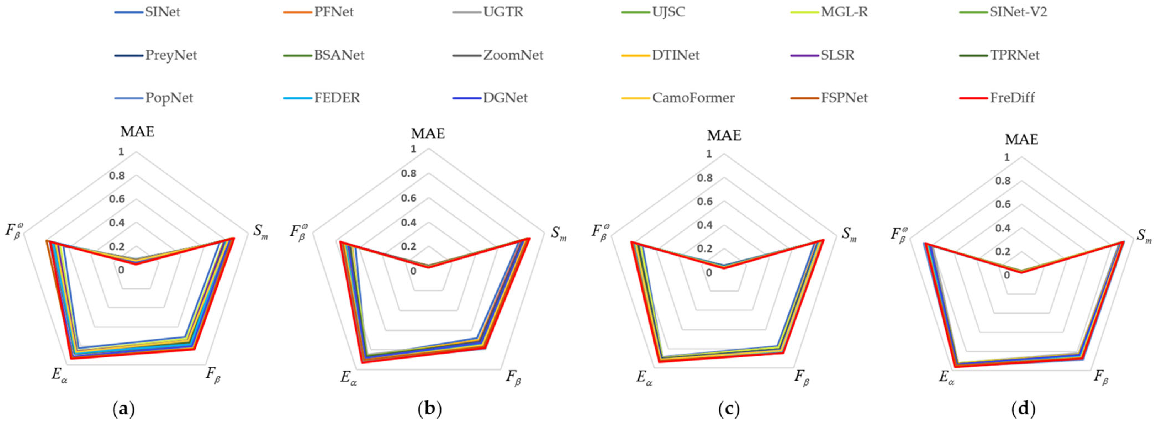
The radar chart on the four datasets is shown in Figure 9, where the values of FreDiff are marked in red. It can be seen that FreDiff achieves overall better performance, which also indicates that this algorithm has stronger generalization ability.

4.4.2. Qualitative Comparison

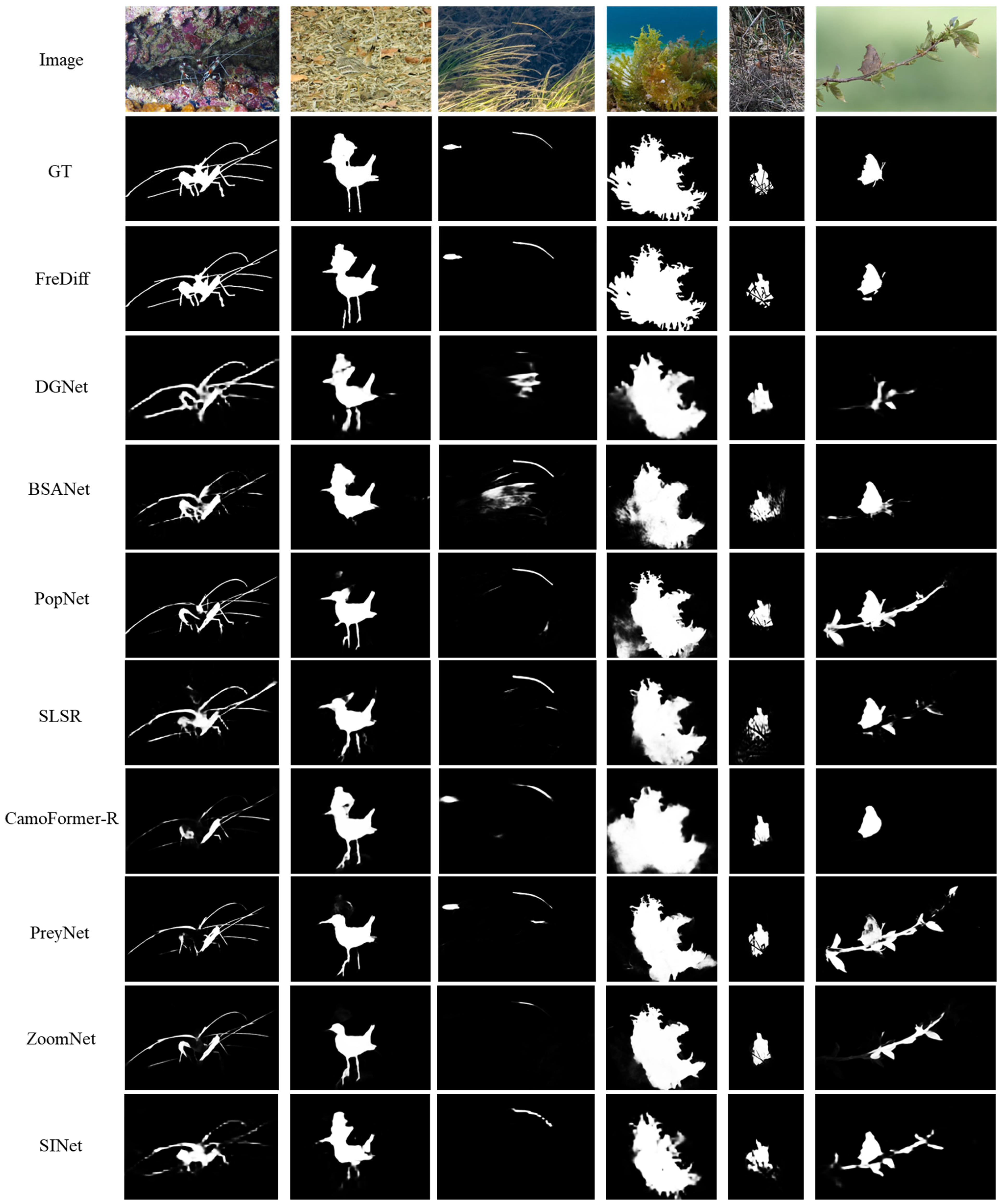
As shown in Figure 10, FreDiff can effectively separate camouflaged targets from the background. FreDiff uses frequency information to assist in feature extraction and then iteratively denoises the camouflaged segmentation map, endowing the model with more complete semantic information. As shown in the fourth column of the figure, other methods are unable to accurately distinguish the camouflaged objects in the image, but our proposed FreDiff can recognize the camouflaged objects completely and clearly, especially the detailed edge information of the targets. Furthermore, we can observe that when there are multiple targets in the third column of images, our method can effectively segment the camouflaged objects among them. GFM provides the rich global information and understanding of contextual relationships, as shown in the last column; FreDiff can segment the camouflaged objects more accurately without being disturbed by non-camouflaged objects.

4.5. Ablation Experiments

In this section, ablation experiments are designed to verify the effectiveness of the key components of FreDiff, including FAM, GFM, UEM, and training strategy. All experiments are conducted on the COD10K dataset, where the baseline network is PVTv2-B3 with a UNet model. The experimental results are shown in

Table 5. Ablation experiment on COD10K dataset.

Baseline	FAM	GFM	UEM	Strategy	MAE↓	${\mathit{S}}_{\mathit{m}}$ ↑	${\mathit{F}}_{\mathit{\beta }}$ ↑	${\mathit{E}}_{\mathit{m}}$ ↑	${\mathit{F}}_{\mathit{\beta }}^{\mathit{\omega }}$ ↑
$\surd$					0.029	0.858	0.767	0.915	0.744
$\surd$	$\surd$				0.027	0.861	0.773	0.912	0.749
$\surd$	$\surd$	$\surd$			0.025	0.863	0.780	0.922	0.753
$\surd$	$\surd$	$\surd$	$\surd$		0.024	0.860	0.780	0.926	0.758
$\surd$	$\surd$	$\surd$	$\surd$	$\surd$	0.024	0.866	0.784	0.929	0.763

The values in bold are the optimal segmentation results, ↑ denotes higher metrics are better and ↓ denotes lower metrics are better.

.

Table 5 comprehensively presents the vertical comparison results of the ablation experiments performed using FreDiff, verifying the effectiveness of each submodule in enhancing model performance through separate testing of FAM, GFM, UEM, and training strategy. It can be observed that compared to the baseline, FreDiff’s performance improves when using FAM, GFM, UEM, and the specific training strategy. Experimental tests were conducted on each module separately. We add FAM to make the network focus on extracting frequency features of images to obtain more comprehensive semantic information, resulting in improvements in five evaluation metrics. After adding GFM, this allows the network to focus more on the global information, reducing the cases of false segmentation to non-camouflaging objects; the $E_m$ improved by 1%. The detail information is enhanced by adding UEM to further distinguish the detail features that are not obvious between the camouflaged object and its environment; the $F_{\beta }$ increased by 1.3% compared to the baseline. The training strategy we designed by changing the noise schedule, and speeds up the process of adding noise so that FreDiff can achieve better segmentation results. The results also show that this method is important to improve the segmentation accuracy.

5. Discussion

The benchmark tests detailed in Section 4 demonstrate that our method has exhibited outstanding efficacy in the field of camouflaged object segmentation. However, several aspects still warrant further discussion.

5.1. Advantages of FreDiff

Although the current COS models have achieved impressive performance, they still exhibit deficiencies in capturing the subtle differences between camouflaged objects and their backgrounds. We propose a camouflaged object segmentation method based on DDPM, named FreDiff. By leveraging frequency information guidance, it extracts more comprehensive information from images, enhancing the model’s feature extraction capabilities and thereby mitigating the issue of blurred boundaries in COS results.

The diffusion model for a COS network can randomly sample from the mask distribution to generate multiple possible prediction results, which helps capture the subtle differences between camouflaged objects and their backgrounds, improving the accuracy and robustness of COS. Furthermore, FreDiff can generate the final segmentation mask by combining the prediction results from multiple sampling steps, alleviating the issue of overconfident point estimates. Through an experimental analysis, FreDiff has been shown to reduce the high false alarm rate for camouflaged objects and achieve clear and accurate segmentation results in complex environments.

5.2. Limitations and Challenge

From the experiments conducted in the previous section, it can be observed that the COS network FreDiff based on the diffusion model outperforms most existing COS models in segmentation performance. However, there are still some issues that need to be addressed. During model training, we found that our model is slower in training speed and requires more computational resources.

Specifically, due to the inherent structural complexity of the diffusion model, a large number of parameters and computations need to be processed during model training to generate high-quality COS mask images. The complexity of the algorithm directly affects the training speed of the model. Furthermore, this is due to the need for thousands of denoising iteration steps during the training process of the diffusion model to gradually refine the sample distribution and generate the optimal COS mask image. This iterative process not only increases computation time but also raises the demand for computational resources. The inference speed of the COS framework based on the diffusion model cannot meet real-time requirements, thereby limiting the wide application of this framework.

Additionally, the size of the input image affects the inference time. The larger the image pixel values, the more pixel points the model needs to process, resulting in a slower training speed for the entire network. The diffusion model for a COS network faces significant computational challenges in high-resolution applications.

Therefore, in the future, we will further investigate how to reduce the complexity and sampling steps of this framework, optimize the computational efficiency of the diffusion model, and conduct research on its lightweighting.

6. Conclusions

This paper proposes a camouflaged object segmentation method based on a diffusion model, which incorporate frequency domain information as auxiliary features, and constructs the FreDiff to address the phenomenon of overconfidence and improve the accuracy of COS. The FAM extracts frequency information from images and we propose FF to better integrate it into the network, thereby obtaining more plentiful image feature information. The GFM focus on global information of the fused features enables the network to understand the contextual information of the image and discern the relationship between camouflaged objects and the background, thereby reducing the likelihood of identifying non-camouflaged objects. The UEM enhances the detailed features of camouflaged objects. This is because the features of camouflaged objects and their backgrounds are highly similar. Enhancing boundary, texture, and other detailed features can improve the accuracy of the COS results and better reveal the details of the objects. Due to the special nature of COS task training, which involves inputting the corresponding ground truth (GT) image into the diffusion model for training, we have designed a linear regularization function to accelerate the noising process, reducing redundant information and enhancing training speed. FreDiff is compared with 17 COS models on four challenging COS datasets, and its performance is superior to or comparable with the best results. Specifically, the metrics of MAE and $E_m$ values outperform other algorithms on all datasets. Finally, we design ablation experiments to demonstrate the effectiveness of each module.

References

1. Fan, D.P.; Ji, G.P.; Sun, G.; Cheng, M.M.; Shen, J.; Shao, L. Camouflaged object detection. In Proceedings of the 2020 IEEE/CVF Conference on Computer Vision and Pattern Recognition (CVPR), Seattle, WA, USA, 13–19 June 2020; pp. 2774–2784. [Google Scholar]
2. Liu, M.Z.; Di, X.G. Extraordinary MHNet: Military high-level camouflage object detection network and dataset. Neurocomputing 2023, 549, 126466. [Google Scholar] [CrossRef]
3. Li, L.; Liu, J.Y.; Wang, S.; Wang, X.K.; Xiang, T.Z. Trichomonas vaginalis segmentation in microscope images. In Proceedings of the Medical Image Computing and Computer Assisted Intervention—MICCAI 2022, Singapore, 18–22 September 2022; Volume 13434, pp. 68–78. [Google Scholar]
4. Tabernik, D.; Sela, S.; Skvarc, J.; Skocaj, D. Segmentation-based deep-learning approach for surface-defect detection. J. Intell. Manuf. 2020, 31, 759–776. [Google Scholar] [CrossRef]
5. Kumar, K.; Rahman, A. Early detection of locust swarms using deep learning. In Advances in Machine Learning and Computational Intelligence; Springer: Berlin/Heidelberg, Germany, 2021; pp. 303–310. [Google Scholar]
6. Jiang, X.H.; Cai, W.W.; Ding, Y.; Wang, X.; Yang, Z.Y.; Di, X.Y.; Gao, W.J. Camouflaged Object Detection Based on Ternary Cascade Perception. Remote Sens. 2023, 15, 1188–1210. [Google Scholar] [CrossRef]
7. Mei, H.; Ji, G.P.; Wei, Z.; Yang, X.; Wei, X.; Fan, D.P. Camouflaged object segmentation with distraction mining. In Proceedings of the 2021 IEEE/CVF Conference on Computer Vision and Pattern Recognition (CVPR), Ithaca, NY, USA, 19–25 June 2021; pp. 8768–8777. [Google Scholar]
8. Fan, D.P.; Ji, G.P.; Cheng, M.M.; Shao, L. Concealed object detection. IEEE Trans. Pattern Anal. Mach. Intell. 2021, 44, 6024–6042. [Google Scholar] [CrossRef] [PubMed]
9. Zhang, M.; Xu, S.; Piao, Y.R.; Shi, D.X.; Lin, S.S.; Lu, H.C. Preynet: Preying on camouflaged objects. In Proceedings of the 30th ACM International Conference on Multimedia (MM), New York, NY, USA, 10–14 October 2022; pp. 5323–5332. [Google Scholar]
10. Pang, Y.; Zhao, X.; Xiang, T.; Zhang, L.; Lu, H. Zoom In and Out: A Mixed-scale Triplet Network for Camouflaged Object Detection. In Proceedings of the 2022 IEEE/CVF Conference on Computer Vision and Pattern Recognition (CVPR), New Orleans, LA, USA, 18–24 June 2022; pp. 2150–2160. [Google Scholar]
11. Wang, W.G.; Lai, Q.X.; Shen, J.B.; Ling, H.B. Salient Object Detection in the Deep Learning Era: An In-depth Survey. IEEE. Trans. Pattern Anal. Mach. Intell. 2019, 44, 3239–3259. [Google Scholar] [CrossRef] [PubMed]
12. Li, A.X.; Zhang, J.; Lv, Y.Q.; Liu, B.; Zhang, T.; Dai, Y.C. Uncertainty-aware Joint Salient Object and Camouflaged Object Detection. In Proceedings of the 2021 IEEE/CVF Conference on Computer Vision and Pattern Recognition (CVPR), Nashville, TN, USA, 19–25 June 2021; pp. 10066–10076. [Google Scholar]
13. Luo, X.J.; Wang, S.; Wu, Z.W.; Sakaridis, C.; Cheng, Y.; Fan, D.P.; Gool, L. CamDiff: Camouflage Image Augmentation via Diffusion. CAAI Artif. Intell. Res. 2023, 2, 915002. [Google Scholar] [CrossRef]
14. Wu, Z.W.; Paudel, D.P.; Fan, D.P.; Wang, J.J.; Wang, S.; Demonceaux, C.; Timofte, R.; Van Gool, L. Source-free Depth for Object Pop-out. In Proceedings of the 2023 IEEE/CVF International Conference on Computer Vision (ICCV), Paris, France, 4–6 October 2023; pp. 1032–1042. [Google Scholar]
15. He, C.M.; Li, K.; Zhang, Y.C.; Tang, L.X.; Zhang, Y.L.; Guo, Z.H.; Li, X. Camouflaged Object Detection with Feature Decomposition and Edge Reconstruction. In Proceedings of the 2023 IEEE/CVF Conference on Computer Vision and Pattern Recognition (CVPR), Vancouver, BC, Canada, 20–22 June 2023; pp. 22046–22055. [Google Scholar]
16. Nichol, A.; Dhariwal, P.; Ramesh, A.; Shyam, P.; Mishkin, P.; McGrew, B.; Sutskever, I.; Chen, M. GLIDE: Towards Photorealistic Image Generation and Editing with Text-Guided Diffusion Models. ICML 2021, 44, 16784–16804. [Google Scholar]
17. Zhang, J.H.; Yan, R.D.; Perell, A.; Chen, X.; Li, C. Phy-Diff: Physics-guided Hourglass Diffusion Model for Diffusion MRI Synthesis. arXiv 2024, arXiv:2406.03002. [Google Scholar]
18. Zhou, H.P.; Wang, H.Q.; Ye, T.; Xing, Z.H.; Ma, J.; Li, P.; Wang, Q.; Zhu, L. Timeline and Boundary Guided Diffusion Network for Video Shadow Detection. arXiv 2024, arXiv:2408.11785. [Google Scholar]
19. Fan, D.P.; Ji, G.P.; Xu, P.; Cheng, M.M.; Sakaridis, C.; Gool, L.V. Advances in Deep Concealed Scene Understanding. Vis. Intell. 2023, 1, 1–24. [Google Scholar] [CrossRef]
20. Le, T.N.; Nguyen, T.V.; Nie, Z.; Tran, M.-T.; Sugimoto, A. Anabranch network for camouflaged object segmentation. Comput. Vis. Image Underst. 2019, 184, 45–56. [Google Scholar] [CrossRef]
21. Lv, Y.; Zhang, J.; Dai, Y.; Li, A.; Liu, B.; Barnes, N. Simultaneously localize; segment and rank the camouflaged objects. In Proceedings of the 2021 IEEE/CVF Conference on Computer Vision and Pattern Recognition (CVPR), Nashville, TN, USA, 20–25 June 2021; pp. 11586–11596. [Google Scholar]
22. Zhang, J.; Lv, Y.Q.; Xiang, M.C.; Li, A.X.; Dai, Y.C.; Zhong, Y.R. Depth confidence-aware camouflaged object detection. In Proceedings of the 2021 IEEE/CVF Conference on Computer Vision and Pattern Recognition (CVPR), Ithaca, NY, USA, 19–25 June 2021; pp. 11641–11653. [Google Scholar]
23. He, R.Z.; Dong, Q.H.; Lin, J.Y.; Lau, R.W. Weakly-supervised camouflaged object detection with scribble annotations. In Proceedings of the Thirty-Seventh AAAI Conference on Artificial Intelligence (AAAI), Washington, DC, USA, 7–14 February 2023; pp. 781–789. [Google Scholar]
24. Pang, Y.W.; Zhao, X.Q.; Xiang, T.Z.; Zhang, L.H.; Lu, H.C. ZoomNeXt: A Unified Collaborative Pyramid Network for Camouflaged Object Detection. IEEE Trans. Pattern Anal. Mach Intell. 2024, 10, 1–16. [Google Scholar] [CrossRef] [PubMed]
25. Ho, J.; Jain, A.; Abbeel, P. Denoising Diffusion Probabilistic Models. In Proceedings of the 34th International Conference on Neural Information Processing Systems (NIPS), Vancouver, BC, Canada, 6–12 December 2020; pp. 6840–6851. [Google Scholar]
26. Wu, J.; Fang, H.; Zhang, Y.; Yang, Y.; Xu, Y. MedSegDiff: Medical Image Segmentation with Diffusion Probabilistic Model. MIDL 2024, 227, 1623–1639. [Google Scholar]
27. Chen, Z.X.; Sun, K.; Liu, X.M.; Ji, R.R. CamoDiffusion: Camouflaged Object Detection via Conditional Diffusion Models. In Proceedings of the AAAI Conference on Artificial Intelligence (AAAI), Washington, DC, USA, 07–14 February 2023; pp. 1272–1280. [Google Scholar]
28. Chen, S.F.; Sun, P.Z.; Song, Y.B.; Luo, P. DiffusionDet: Diffusion Model for Object Detection. In Proceedings of the 2023 IEEE/CVF International Conference on Computer Vision (ICCV), Paris, France, 2–6 October 2023; pp. 19773–19786. [Google Scholar]
29. Xu, K.; Qin, M.H.; Sun, F.; Wang, Y.H.; Chen, Y.K.; Ren, F.B. Learning in the Frequency Domain. In Proceedings of the 2020 IEEE/CVF Conference on Computer Vision and Pattern Recognition (CVPR), Seattle, WA, USA, 13–19 June 2020; pp. 1737–1746. [Google Scholar]
30. Zhong, Y.J.; Li, B.; Tang, L.; Kuang, S.Y.; Wu, S.; Ding, S.H. Detecting Camouflaged Object in Frequency Domain. In Proceedings of the 2022 IEEE/CVF Conference on Computer Vision and Pattern Recognition (CVPR), New Orleans, LA, USA, 19–20 June 2022; pp. 4494–4503. [Google Scholar]
31. Cong, R.M.; Sun, M.Y.; Zhang, S.Y.; Zhou, X.F.; Zhang, W.; Zhao, Y. Frequency Perception Network for Camouflaged Object Detection. In Proceedings of the 34th International Conference on Neural Information Processing Systems (NIPS’20), Vancouver, BC, Canada, 6–12 December 2020; pp. 1179–1189. [Google Scholar]
32. Dong, B.; Wang, P.C.; Wang, F. Head-Free Lightweight Semantic Segmentation with Linear Transformer. In Proceedings of the AAAI Conference on Artificial Intelligence (AAAI), Washington, DC, USA, 7–14 February 2023; pp. 516–524. [Google Scholar]
33. Wang, W.H.; Xie, E.; Li, X.; Fan, D.P.; Song, K.T.; Liang, D.; Lu, T.; Luo, P.; Shao, L. PVT v2: Improved baselines with Pyramid Vision Transformer. Comput. Vis. Media 2022, 8, 415–424. [Google Scholar] [CrossRef]
34. Hoogeboom, E.; Heek, J.; Salimans, T. Simple diffusion: End-to-end diffusion for high resolution images. arXiv 2023, arXiv:2301.11093. [Google Scholar]
35. Le, T.N.; Cao, Y.B.; Nguyen, T.C.; Do, T.T.; Tran, M.T.; Nguyen, T.V. Camouflaged instance segmentation in-the-wild: Dataset, method, and benchmark suite. IEEE Trans. Image Process. 2022, 31, 287–300. [Google Scholar] [CrossRef]
36. Skurowski, P.; Abdulameer, H.; Błaszczyk, J.; Depta, T.; Kornacki, A.; Przemysław, K. Animal camouflage analysis: Chameleon database. Unpubl. Manuscr. 2018, 2, 7. [Google Scholar]
37. Perazzi, F.; Krähenbühl, P.; Pritch, Y.; Hornung, A. Saliency filters: Contrast based filtering for salient region detection. In Proceedings of the 2012 IEEE Conference on Computer Vision and Pattern Recognition (CVPR), Providence, RI, USA, 16–21 June 2012; pp. 733–740. [Google Scholar]
38. Fan, D.P.; Cheng, M.M.; Liu, Y.; Li, T.; Borji, A. Structure-measure: A new way to evaluate foreground maps. In Proceedings of the 2017 IEEE International Conference on Computer Vision (ICCV), Ithaca, NY, USA, 22–29 October 2017; pp. 4558–4567. [Google Scholar]
39. Margolin, R.; Zelnik-Manor, L.; Tal, A. How to evaluate foreground maps. In Proceedings of the 2014 IEEE Conference on Computer Vision and Pattern Recognition (CVPR), Ithaca, NY, USA, 23–28 June 2014; pp. 248–255. [Google Scholar]
40. Fan, D.P.; Gong, C.; Cao, Y.; Ren, B.; Cheng, M.M.; Borji, A. Enhanced-alignment measure for binary foreground map evaluation. In Proceedings of the Twenty-Seventh International Joint Conference on Artificial Intelligence, Ithaca, NY, USA, 18–22 June 2018; pp. 698–704. [Google Scholar]
41. Yang, F.; Zhai, Q.; Li, X.; Huang, R.; Luo, A.; Cheng, H.; Fan, D.P. Uncertainty-Guided Transformer Reasoning for Camouflaged Object Detection. In Proceedings of the 2021 IEEE/CVF International Conference on Computer Vision (ICCV), Montreal, QC, Canada, 11–17 October 2021; pp. 4126–4135. [Google Scholar]
42. Zhai, Q.; Li, X.; Yang, F.; Chen, C.Z.; Cheng, H.; Fan, D.P. Mutual Graph Learning for Camouflaged Object Detection. In Proceedings of the 2021 IEEE/CVF Conference on Computer Vision and Pattern Recognition (CVPR), Nashville, TN, USA, 19–25 June 2021; pp. 12992–13002. [Google Scholar]
43. Zhu, H.W.; Li, P.; Xie, H.R.; Yan, X.F.; Liang, D.; Chen, D.P.; Wei, M.Q.; Qin, J. I Can Find You! Boundary-Guided Separated Attention Network for Camouflaged Object Detection. AAAI 2022, 36, 3608–3616. [Google Scholar] [CrossRef]
44. Liu, Z.; Zhang, Z.L.; Wu, W. Boosting Camouflaged Object Detection with Dual-Task Interactive Transformer. In Proceedings of the 26th International Conference on Pattern Recognition (ICPR), Montreal, QC, Canada, 21–25 August 2022; pp. 140–146. [Google Scholar]
45. Lv, Y.Q.; Zhang, J.; Dai, Y.C.; Li, A.X.; Barnes, N.; Fan, D.P. Toward Deeper Understanding of Camouflaged Object Detection. IEEE Trans. Circuits Syst. Video Technol. 2022, 33, 3462–3476. [Google Scholar] [CrossRef]
46. Zhang, Q.; Ge, Y.; Zhang, C.; Bi, H.B. TPRNet: Camouflaged object detection via transformer-induced progressive refinement network. Visual Comput. 2022, 39, 4593–4607. [Google Scholar] [CrossRef]
47. Ji, G.P.; Fan, D.P.; Chou, Y.C.; Dai, D.; Liniger, A.; Van Gool, L. Deep Gradient Learning for Efficient Camouflaged Object Detection. Mach. Intell. Res. 2023, 20, 92–108. [Google Scholar] [CrossRef]
48. Yin, B.; Zhang, X.; Hou, Q.; Sun, B.Y.; Fan, D.P.; Van Gool, L. CamoFormer: Masked Separable Attention for Camouflaged Object Detection. IEEE Trans. Pattern Anal. Mach. Intell. 2024, 14, 1–14. [Google Scholar] [CrossRef] [PubMed]
49. Huang, Z.; Dai, H.; Xiang, T.-Z.; Wang, S.; Chen, H.-X.; Qin, J.; Xiong, H. Feature Shrinkage Pyramid for Camouflaged Object Detection with Transformers. In Proceedings of the 2023 IEEE/CVF Conference on Computer Vision and Pattern Recognition (CVPR), Vancouver, BC, Canada, 20–22 June 2023; pp. 5557–5566. [Google Scholar]
Figure 1. The paradigm of camouflaged object segmentation. (a) The normal COS paradigm inputs images into the network for mask prediction. (b) The diffusion model for the COS paradigm inputs images through the backbone to obtain features, and then utilizes the diffusion model to iteratively refine the noisy GT image, ultimately generating the mask prediction.
Electronics 13 03922 g001
Figure 2. Difference between camouflaged object and general object.
Electronics 13 03922 g002
Figure 3. The diffusion process of DDPM for COS.
Electronics 13 03922 g003
Figure 4. Frequency-guided COS network based on diffusion model (FreDiff) structure. (a) FreDiff structure. (b) Backbone PVTv2 structure.
Electronics 13 03922 g004aElectronics 13 03922 g004b
Figure 5. Frequency auxiliary module (FAM) structure.
Electronics 13 03922 g005
Figure 6. Global Fusion Module (GFM) structure.
Electronics 13 03922 g006
Figure 7. Upsample Enhancement Module (UEM) structure.
Electronics 13 03922 g007
Figure 8. Curves on the four COS datasets.
Electronics 13 03922 g008
Figure 9. Radar plots for the evaluation metrics on the four COS datasets. (a) CAMO; (b) COD10K; (c) NC4K; (d) CHAMELEON.
Electronics 13 03922 g009
Figure 10. Visual comparison results of camouflaged object segmentation maps with other methods.
Electronics 13 03922 g010