Abstract
Video anomaly detection is a critical component of intelligent video surveillance systems,
extensively deployed and researched in industry and academia. However, existing methods have a
strong generalization ability for predicting anomaly samples. They cannot utilize high-level semantic
and temporal contextual information in videos, resulting in unstable prediction performance. To
alleviate this issue, we propose an encoder–decoder model named SMAMS, based on spatiotemporal
masked autoencoder and memory modules. First, we represent and mask some of the video events
using spatiotemporal cubes. Then, the unmasked patches are inputted into the spatiotemporal
masked autoencoder to extract high-level semantic and spatiotemporal features of the video events.
Next, we add multiple memory modules to store unmasked video patches of different feature layers.
Finally, skip connections are introduced to compensate for crucial information loss caused by the
memory modules. Experimental results show that the proposed method outperforms state-of-the-art
methods, achieving AUC scores of 99.9%, 94.8%, and 78.9% on the UCSD Ped2, CUHK Avenue, and
Shanghai Tech datasets.
1. Introduction
In recent years, with the widespread application of video surveillance and municipal management, anomaly detection has gained extensive attention in video surveillance, which plays an indispensable role in ensuring public and personal safety. Video anomaly detection (VAD) refers to identifying events in a video that deviate from expected behavior. Despite many endeavors, VAD is still highly challenging for three main reasons: (1) The rarity of anomalous events results in an imbalance between normal and abnormal samples. (2) The unpredictability of anomalous events makes it difficult for researchers to collect all such events. (3) The ambiguity in defining anomalous events can result in the same behavior having completely different anomalous properties in different scenarios. For example, running in the middle of the road is considered abnormal, while running in the park is normal. Therefore, it becomes impractical to construct a VAD task using traditional supervised video event classification techniques. VAD is typically regarded as an outlier detection problem, in which a normal model is trained using normal data, and events that deviate from the normal model are detected as anomalies during testing.
When it comes to detecting anomalies in videos, there are two main approaches: traditional and deep-learning-based. Traditional methods rely on handcrafted features that represent the video’s appearance and motion [1,2]. However, these methods are labor-intensive, require meticulous manual design, and can be difficult to extract practical feature information. Lately, the field of VAD has been largely influenced by deep learning methodologies. These techniques can be categorized into two subdivisions: reconstruction-based and prediction-based approaches. Reconstruction-based methods [3,4,5] use normal events to train autoencoders and use the learned features to reconstruct input data. In testing, events that exhibit larger reconstruction errors are deemed to be anomalous. However, the strong generalization capability of the autoencoder can effectively reconstruct anomalies as well [3]. In other words, as the network depth of these autoencoders increases, they become proficient at reconstructing both normal and abnormal samples, leading to reduced distinguishability between normal and abnormal events due to similar reconstruction errors. This limitation arises from the excessive focus on low-level details and the neglect of higher-level semantic information in existing methods [6]. The prediction-based methods [7,8,9] aim to predict future frames based on past frames. If the prediction of the future frame significantly deviates from the actual ground truth, it is a clear indication of anomalies. However, due to the minimal changes in temporal and spatial features of adjacent frames, prediction methods can better predict future frames based on past frames, even for abnormal samples. This limitation is because prediction methods based on single-frame prediction errors cannot fully utilize the temporal and spatial context of video abnormal activities when predicting anomalies [10,11,12]. The limitations of these two methods in extracting advanced visual features and comprehensive temporal-spatial contextual relationships hinder their further performance enhancement.
In this paper, our goal is to explore better methods to mine the high-level semantics and complex spatiotemporal relationships of video events. Initially, we represented video events using spatiotemporal cubes (STCs), which are constructed from consecutive foreground segments in unlabeled videos. This allows us to deeply explore the spatiotemporal characteristics of the video content, facilitating a more comprehensive understanding and analysis of the video events. Subsequently, the foreground patches are randomly masked, and the unmasked patches are fed into a spatiotemporal mask autoencoder, which aims to learn the spatiotemporal features of video events. By randomly masking the foreground patches, the autoencoder is forced to reconstruct the occluded regions, enabling it to capture the spatiotemporal features more accurately in the video. By leveraging the ability of autoencoders to learn inherent structures and patterns from data, it can extract high-level semantic and spatiotemporal features that are useful for comprehensively understanding and analyzing video events. Furthermore, to better reconstruct normal events and worse abnormal events, we introduce multiple memory modules between the spatiotemporal masked autoencoders. These modules store the typical patterns of unmasked video patches from distinct feature layers. In addition, to compensate for the loss of key information caused by the memory modules, we also added skip connections to ensure a more complete reconstruction of both normal and abnormal events. Finally, the reconstructed masked video data are obtained from the decoding module, and the normal score for each input is obtained based on the differences between the reconstructed data and the input data.
In summary, we propose an encoder–decoder model named SMAMS, based on spatiotemporal masked autoencoder (ST-MAE) and memory modules. The main contributions of this paper are summarized as follows:
- (1)
- Using the spatiotemporal cubes (STCs) to represent video events, we can explore the spatiotemporal characteristics of video content in depth, facilitating a more comprehensive understanding and analysis of video events.
- (2)
- By learning the spatiotemporal features of video events through a spatiotemporal mask autoencoder, it accurately captures the spatiotemporal features in video and extracts advanced semantic and spatiotemporal features that are helpful for comprehensive understanding and analysis.
- (3)
- Introducing multiple memory modules and skipping connections to better reconstruct normal and abnormal events, compensate for the loss of key information, ensure a more complete reconstruction, and obtain normal scores based on the differences between reconstructed data and input data.
- (4)
- Our model demonstrated competitive performance on three datasets: UCSD Ped2, CUHK Avenue, and Shanghai Tech. Furthermore, we conducted comprehensive ablation experiments to investigate the impact of various model components.
2. Related Work
2.1. Video Anomaly Detection (VAD)
Reconstruction-based methods typically learn to reconstruct the input by training on normal videos and consider those with a large reconstruction error as anomalies. Autoencoders (AE) and their variants are widely used for reconstructing training data. Gong et al. [3] proposed a Memory-Augmented Autoencoder (MemAE) to address the limitations of traditional autoencoders in anomaly detection. Fan et al. [13] implemented VAD using a Gaussian mixture variational autoencoder. Recently, several relevant studies have delved into the application of residual networks in autoencoders. Deepak et al. [14] introduced a residual spatiotemporal autoencoder that addresses the issue of gradient vanishing in traditional convolutional autoencoders by incorporating skip connections and residual blocks into its architecture. Le et al. [4] presented a residual autoencoder architecture that incorporates a deep convolutional neural network-based encoder and a decoder equipped with multi-level channel attention. Kommanduri et al. [15] proposed a Bi-Residual AutoEncoder that employs dual residual connections to preserve both local and global information. Some works combine LSTM with autoencoders. Wei et al. [5] proposed an autoencoder architecture based on a stacked convolutional LSTM framework to train normal patterns. Joshi et al. [16] proposed an LSTM-based autoencoder architecture that can reconstruct features extracted by a CNN model. Waseem et al. [17] introduced a convolutional LSTM architecture that integrates a variational autoencoder, with the bottleneck layer representing the distribution of mean and variance. A dual-stream framework is popular for detecting video anomalies by combining appearance and motion anomalies. For example, Li et al. [18] employed both a Space–Time Adversarial Autoencoder and a Space–Time Convolutional Autoencoder to fuse the appearance and motion cues of video anomaly events for a more comprehensive evaluation of anomalies. Li and Chen et al. [19] proposed a novel dual-stream architecture called Two-Stream Deep Space–Time Autoencoder (Two-Stream DSTAE) to extract appearance features and motion patterns separately and fuse them with a joint reconstruction error strategy to extract spatiotemporal features for anomaly detection. To address the issue of the lack of exploration of correlation in the dual-stream framework, Liu et al. [20] proposed a dual-stream autoencoder framework based on enhanced space–time memory, which explores the correlation between spatial and temporal patterns through adversarial learning to boost anomaly detection performance. The reconstruction-based methods tend to overemphasize low-level details rather than delve into high-level semantics, resulting in excessive generalization that hinders effective discrimination between normal and abnormal samples.
Prediction-based approaches construct the present frame by learning from earlier frames, and if the prediction result is not satisfactory, it is considered an anomaly. Liu et al. [8] modeled video sequences using deep learning models and used a generative model to predict frames. The first work detected anomalous events using the difference between predicted and actual future frames. Building on this work, Lu et al. [9] proposed an improved approach considering temporal information in predicting future frames from a modeling perspective. They proposed a generative model based on the variational autoencoder (VAE) and Convolutional LSTM (ConvLSTM). Wang et al. [21] designed a multi-path ConvGRU frame prediction module to better handle semantic information in different regions and capture the spatiotemporal dependencies of normal videos. Zhao et al. [22] utilized the evolution laws of long-term and short-term appearance and motion to utilize the spatiotemporal correlations between video frames better to understand normal patterns. Xu et al. [23] introduce a motion-aware future frame prediction network that integrates salient detection with frame prediction branches for effective anomaly detection in videos. Baradaran et al. [24] present a future frame prediction proxy task and semantic segmentation map to effectively address the challenges of long-term motion modeling in VAD. Deng et al. [25] utilize optical flow estimation and interpolation networks to synthesize normal frames and detect anomalies. Cheng et al. [26] proposed a flow-frame prediction model based on spatial-temporal graph convolutional networks, combined with appearance and motion features, for detecting video anomalies. In addition, some recent works have utilized Generative Adversarial Networks (GANs) for future frame prediction. Li et al. [27] proposed an anomaly detection method based on a Generative Adversarial Network with an auxiliary discriminator, which combined adversarial and collaborative prediction of future frames for anomaly detection. Zhang et al. [28] proposed an unsupervised anomaly detection method based on Generative Adversarial Networks (GANs), which utilized two generators to predict the next future frame. However, these methods fail to fully utilize the temporal context of abnormal activities in videos.
Both reconstruction-based and prediction-based methods have their limitations and cannot provide a flawless solution. We propose a VAD method that uses a masked autoencoder with spatiotemporal capabilities, combined with multi-memory and skip connections, to extract high-level semantic and spatiotemporal context information from video events.
2.2. Memory Modules
Memory modules can enhance the network to remember and learn complex information better and have attracted increasing attention for their better performance in various tasks. A differentiable neural computer model was put forward by Graves et al. [29] and consists of a memory module for external data storage and a neural network for feature extraction. Gong et al. [3] introduced the Memory-Enhanced Autoencoder (MemAE) method, which reconstructs outputs by retrieving similar memory slots and combining them to generate new encoding features. This method stores normal patterns in the memory storage, suppressing the autoencoder’s generalization ability. Following this trend, Park et al. [30] presented an inferior memory module that may be updated while being tested. To overcome the limitations of current neural memory networks in knowledge retrieval mechanisms, Fernando et al. [31] proposed a plastic neural memory access mechanism. This mechanism dynamically adjusts connection weights to adapt to different input data, therefore improving the flexibility and efficiency of neural memory networks in knowledge retrieval and output generation. Yu et al. [32] proposed a novel long-term segmentation and tracking method, LTST, aimed at addressing the limitation of existing video object segmentation tasks in creating target models in the first frame, therefore improving long-term adaptability. The proposed method employs a memory attention network to extract relevant historical information and dynamically reconstruct the segmentation template, achieving the effect of online learning. We propose a multi-layer Memory-Enhanced Autoencoder to store critical features of distinct feature layers and add skip connections to compensate for the information loss caused by the memory module.
3. The Proposed SMAMS Video Anomaly Detection Approach
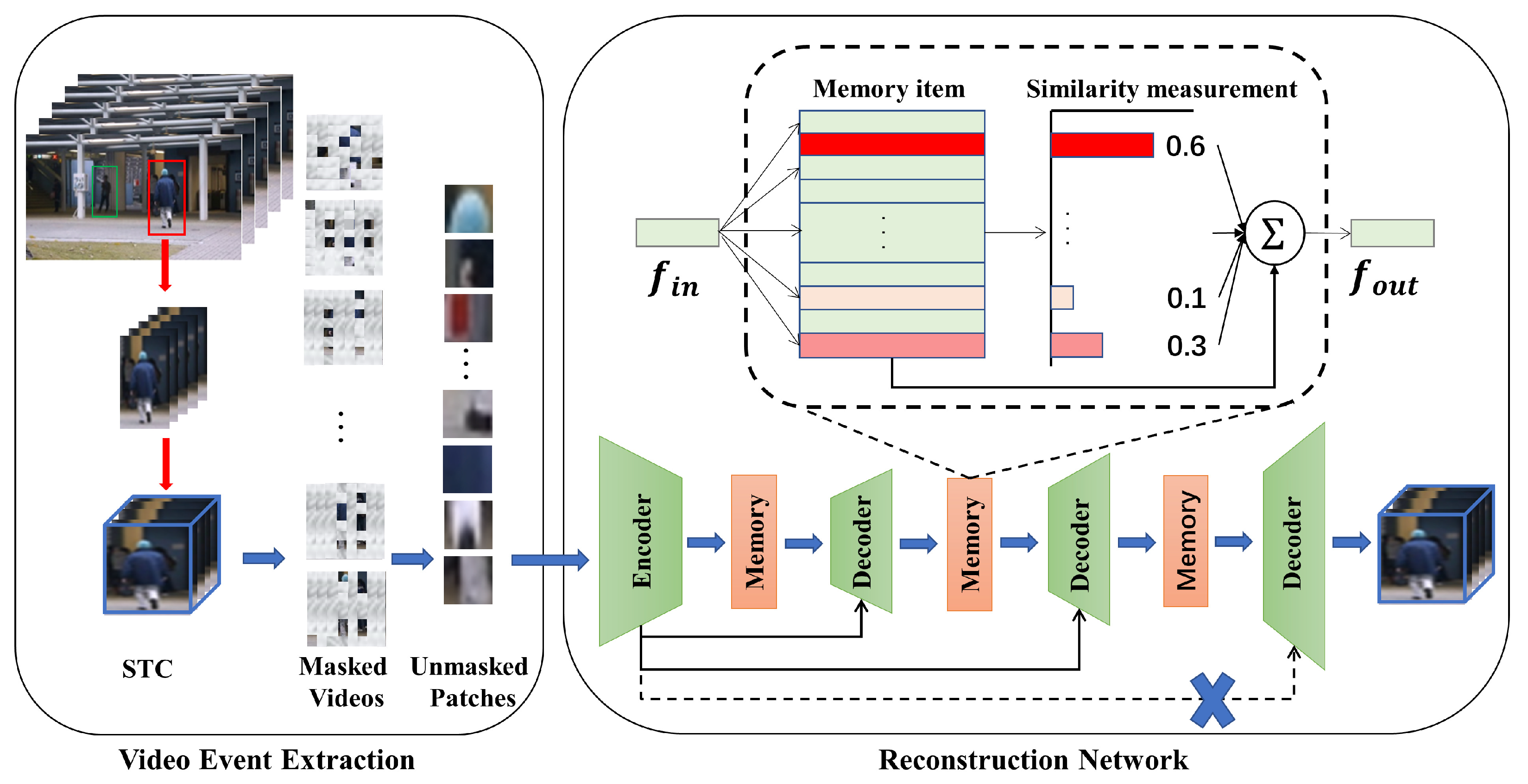
To address the problem of the strong generalization ability to exist methods for predicting abnormal samples, which cannot utilize advanced semantics, we propose an encoder–decoder model, named SMAMS, which is based on a spatiotemporal masked autoencoder (ST-MAE), incorporating multi-memory and skip connections. The network of our method is shown in Figure 1. Initially, the video events are represented as spatiotemporal cubes, and a portion of the foreground patches are randomly concealed. Subsequently, the unmasked patches were fed into the spatiotemporal masked autoencoder, which can extract both the spatiotemporal features and high-level semantics of the video events. Second, to reconstruct normal events better and abnormal events worse, multiple memory modules are added on top of the spatiotemporal masked autoencoder to store the normal patterns of uncovered video patches from different feature layers. Additionally, skip connections are added to compensate for the crucial feature loss caused by the memory modules. Normal event patterns are commonly characterized by simplicity and predictability, whereas abnormal event patterns tend to exhibit greater complexity and irregularity. Finally, the reconstructed masked video data are obtained from the decoding module, and the normal score for each input is obtained based on the differences between the reconstructed data and the input data.
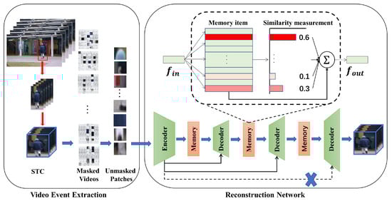
Figure 1.
The network of our method, SMAMS.
3.1. ST-MAE Based Memory Encoder–Decoder
Traditional convolutional autoencoders have a poor temporal dependency. To better utilize the advanced semantics and temporal contextual cues of video events, we introduce the spatiotemporal masked autoencoder (ST-MAE) into the field of VAD. ST-MAE is a novel method for reconstructing the training dataset, which can be used for denoising and fully learning high-level semantics and spatiotemporal features of normal samples.
Spatial-temporal cubes (STC) are used in our proposed method to represent video events, which are constructed from temporally contiguous foreground patches. STC extraction is critical for detecting anomalies [33,34] since it allows subsequent modeling to concentrate on relevant foreground information instead of unimportant backgrounds in video clips. We first localize every frame in the video to gather the foreground information, adopting the video event extraction approach in [34,35]. Second, according to each object’s position, T foreground blocks are taken from the present frame and T-1 subsequent frames in time. Finally, the size of the T foreground patches is adjusted to , and then heaped to generate a STC, . Given a video event represented by the STC , randomly conceal 90% of the foreground patches. Assuming the masked spatiotemporal patches are , . The unmasked spatiotemporal patches are , . We follow the settings of ST-MAE and use ViT as the backbone network for the encoder and decoder. The unmasked spatiotemporal patch sequence is input to the encoder for encoding, resulting in a hidden feature y. The feature representation y can be utilized as the query to retrieve and modify items within the memory module.
where and represent hyperparameters, and represents the memory module’s output feature representation. The decoder is used to reconstruct the masked spatiotemporal patches.
where represents the hyperparameters of the decoder .
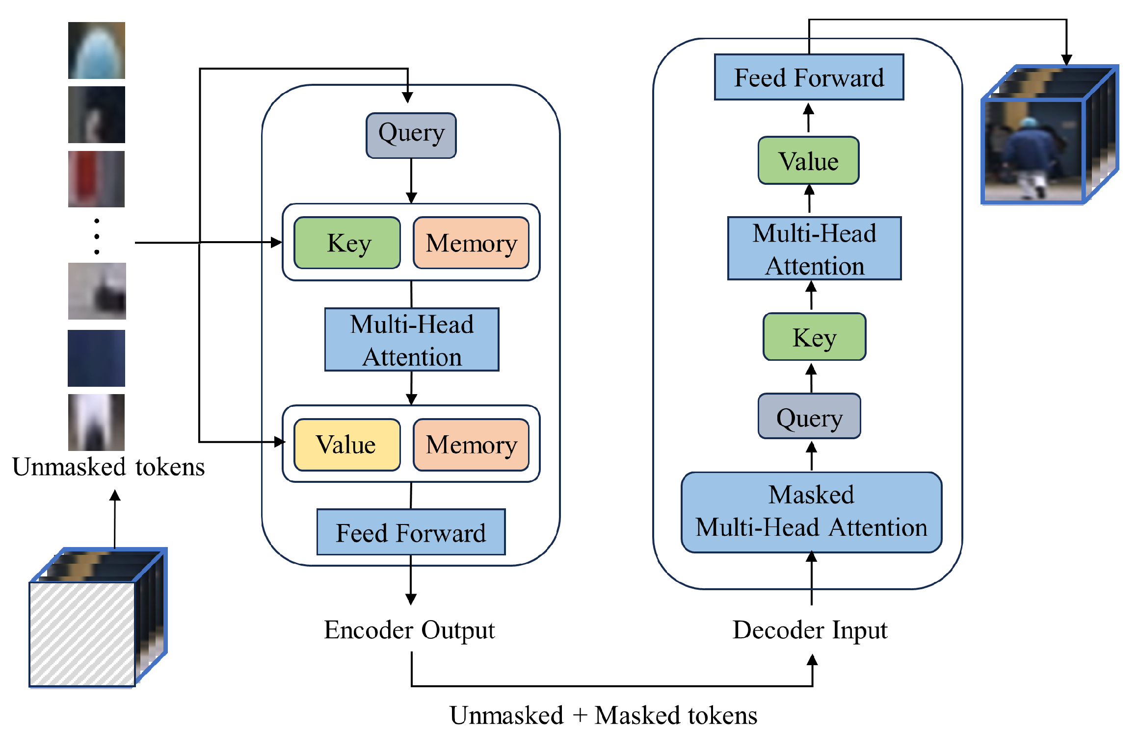
In particular, we adopt the ST-MAE model combined with the memory module as the backbone of our masked autoencoder. As shown in Figure 2, the encoder utilizes the Transformer architecture and memory module, composed of multiple self-attention layers and feed-forward neural network layers and memory module. The decoder part is mainly responsible for reconstructing the input-masked blocks according to the original settings of the Transformer. In VAD, ST-MAE effectively models the temporal and spatial correlations in video sequences, leading to a better understanding of the differences between normal and abnormal patterns. The memory module is to remember the normal mode of unmasked patches. Specifically, the unmasked spatiotemporal patches are used as the input to the encoder part. Given the sequence of unmasked patches , it is first flattened into a 1-dimensional token sequence . Each token sequence is then mapped to a lower-dimensional embedding using a trainable linear projection. To preserve the spatiotemporal information of the patches, learnable embeddings and learnable position embeddings are added to the token embeddings, resulting in the following token sequence:
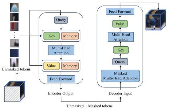
Figure 2.
The internal structure of the masked autoencoder.
Then, we pass the token sequence through multiple encoder blocks, where each block performs the following computation processes to learn temporal-spatial features f of unmasked patches.
where is the encoder input matrix formed from the unmasked patches. and are the input and output of layer l, , , are the linear projections of the encoder’s layer l-1 for query, key, and value of the multi-head attention operator, respectively. , are the layer l learnable memory matrices that are concatenated with , . The multi-head attention operator adheres to the standard architecture of ViT and Transformer. L represents the count of encoder blocks. Multiple encoders can be stacked together to form a deep architecture, therefore increasing the model’s representative capacity. Based on our experiments and evaluations, we have determined that setting L to 3 yields the optimal configuration for our model.
Subsequently, the decoder is employed to reconstruct the sequence of masked patches. The generated STC is considered to be the reconstruction of the original sequence . The ST-MAE is trained by minimizing the reconstruction error.
3.2. Multi-Layer Memory Module with Skip Connections
First, the memory module is introduced, which consists of two main components: an encoding pattern that provides query and matching for memory item storage features and a memory update strategy. By utilizing a memory module, the model can effectively prevent the reconstruction of anomalous samples, significantly improving anomaly detection performance. During the query and match phase, the memory module is designed as a matrix , where it consists of N feature vectors of dimension C. The memory matrix M stores the normal patterns observed during the training process. Assuming the dimension of the feature representation z is the same as C, . Let the row vector represent a memory item in the matrix M, where i denotes the i- row of matrix M. Given a query feature , we can retrieve similar memory items and reconstruct the feature by multiplying them with .
where represents the similarity between the query feature z and the memory items, which can be mathematically expressed as follows:
where represents the cosine similarity:
For the memory update strategy, the following metrics are utilized to gauge the matching degree between memory items and queries:
Each memory item is updated to:
where represents the norm, and the weighted average of the feature is computed to make the feature pattern in the memory item more normal. We adopted the approach proposed in reference [36], where three memory modules were introduced between the encoder and decoder of the spatiotemporal masking autoencoder. These memory modules were designed to capture the features of unmasked patches. Additionally, skip connections were incorporated to ensure the preservation of crucial information.
3.3. Anomaly Score
After performing the ST-MAE, we aim to distinguish anomalies by computing an anomaly score. Following existing reconstruction-based methods, we use reconstruction error as the anomaly score. Let the reconstruction result for be denoted as , and we employ the mean squared error (MSE) loss as the reconstruction loss for each STC:
where represents the norm. It calculates the Euclidean distance between the predicted values and the true values . A higher value implies a greater differentiation between the predicted values and the true values.
The matching probability w for each memory module is added with entropy loss as the memory module loss:
where M is the number of memory modules and is the matching probability for the j-th memory slot in the i-th memory module. Balancing the above two loss functions, we obtain the following loss function to train the model:
In the testing phase, we utilize the trained autoencoder model to reconstruct the test data and calculate the loss error for each sample. For each STC, the anomaly score is computed pixel-wise based on the defined loss function. It can be calculated as follows:
where and represent the mean and standard deviation of the losses ℓ. The anomaly score represents the distribution of reconstruction errors for a sample relative to normal behavior. A higher anomaly score indicates a larger deviation of the sample from normal behavior, suggesting the presence of anomalies.
4. Experiments
4.1. Datasets and Evaluation Metrics
Datasets. We conduct experimental validation on three publicly available datasets: UCSD Ped2 [2], CUHK Avenue [37], and Shanghai Tech [38]. The UCSD Ped2 dataset consists of pedestrian walking videos captured on sidewalks, comprising 28 video clips. Among them, 16 video sequences depict normal pedestrian behavior, while the remaining 12 video sequences contain anomalous behavior such as cycling, driving small cars, and riding skateboards. The CUHK Avenue dataset features videos captured from a horizontal perspective at subway entrances, comprising 37 video clips. Among them, 16 video sequences depict normal pedestrian behavior, while the remaining 21 video sequences contain anomalous behavior such as running and throwing litter. The ShanghaiTech dataset is highly challenging and is the largest dataset in existing benchmarks for anomaly detection, containing over 270,000 training frames and 130 abnormal events. Normal events observed on the campus primarily consist of pedestrians engaged in normal walking behavior. On the other hand, abnormal events encompass a range of occurrences, such as vehicles unlawfully traversing sidewalks, instances of violent altercations, and incidents of robbery.
Evaluation Metrics. We measure the model’s overall performance by calculating the area under the receiver operating characteristic (ROC) curve (AUC). This metric provides a comprehensive assessment of the anomaly detection capabilities of our proposed method. When evaluating the performance of a classification model, we also utilize commonly used evaluation metrics, the F1 score and OA (Overall Accuracy).
4.2. Implementation Details
The implementation details are as follows. We utilize Cascade R-CNN, which is based on mm detection, to extract the foreground objects. These extracted objects are then stacked to build STCs. The size of the STC is set to D = 8, and the width and height of the STCs are adjusted to H = W = 32. We employ a spacetime-agnostic masking strategy to conceal part of the STCs, with a mask ratio set to 0.9. The unmasked STC is used to train our model, while the masked STC is used for model reconstruction. For the ViT module in SMAMS, we set the number of ViT blocks to L = 4 and the embedding dimension dim = 512. At the same time, the number of heads in MSA is set to 8, and the hidden dimension in MLP is 1024. We use 3 memory modules, with N = 2000 for each memory module. The optimizer uses the Adam optimizer in PyTorch with a learning rate of 0.0001. The batch size is 128, and the training epoch is 200. and are set to 1.0 and 0.0002, respectively. The anomaly scores of videos are smoothed by a median filter with a window size of 16.
4.3. Ablation Experiments
4.3.1. The Impact of Different Cube Sizes on Model Performance
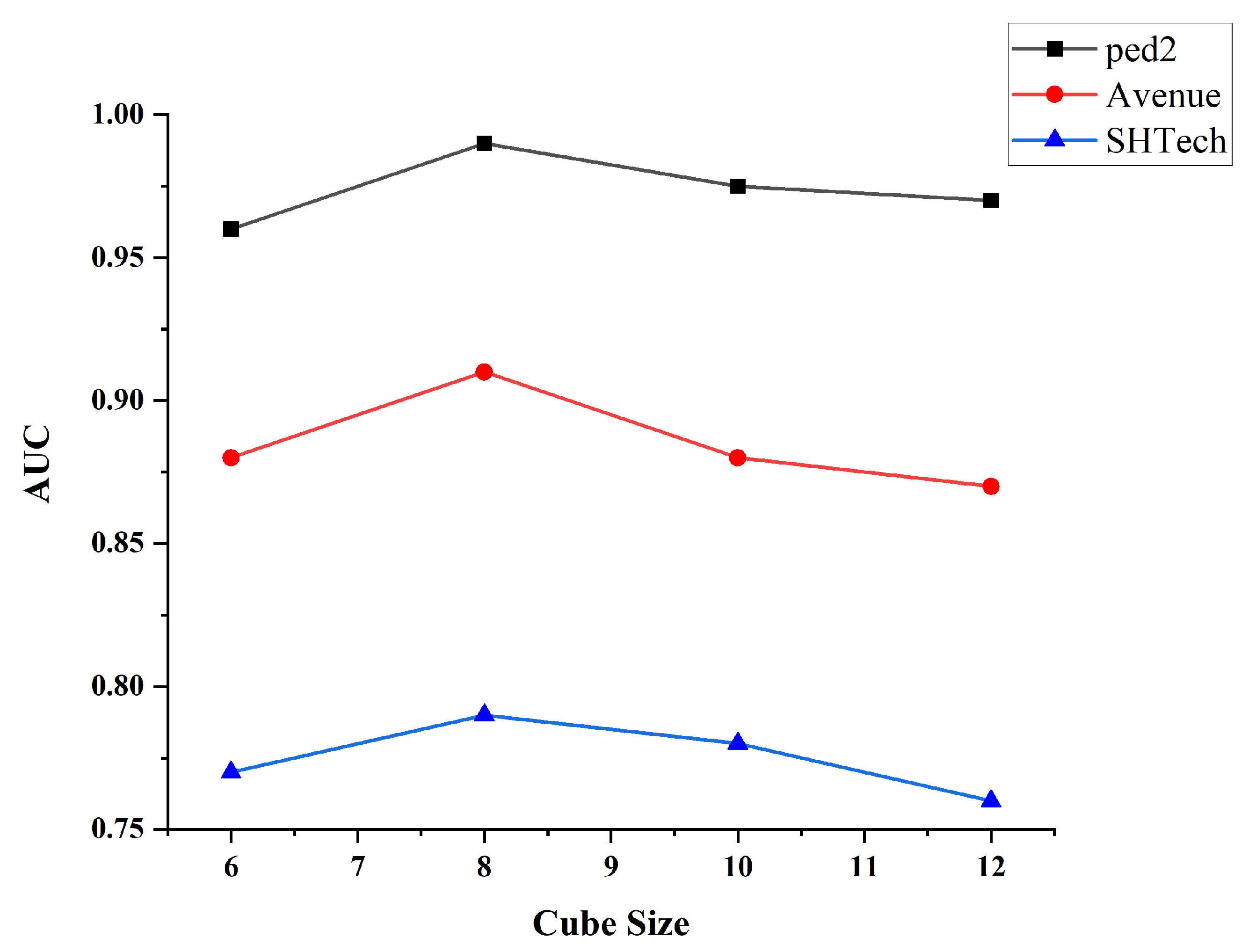
The setting of different cube sizes in ST-MAE can affect the model’s performance, as shown in Figure 3. Cube sizes that are too large or too small can affect the model’s generalization ability and stability. We conducted experiments using different cube sizes and found that the model’s performance was optimal when the cube size was set to 8.
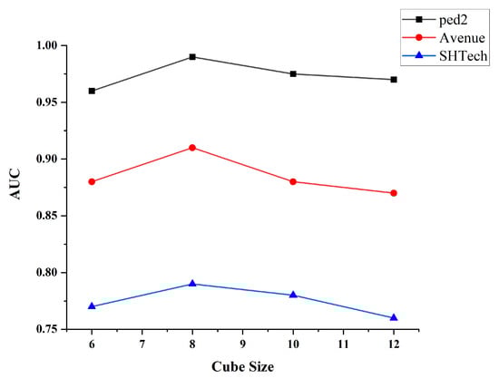
Figure 3.
The impact of different cube sizes on model performance.
4.3.2. Design of Hyperparameters for the Model
In our experiments, we found that the design of the model is a crucial aspect in determining the performance of the SMAMS model.
The choice of an appropriate patch size is crucial for capturing spatial and temporal dependencies. Smaller patch sizes are well-suited for capturing short-term temporal features and local spatial features, making them highly effective in detecting rapidly changing anomalies in local regions. Conversely, larger patch sizes are more suitable for capturing long-term temporal dependencies and global spatial features, which are beneficial for gradually detecting changing global anomalies over time. For our anomaly detection task, our experimental results indicate that setting the patch size to 16 × 16 yields the best performance, as shown in Table 1.

Table 1.
Patch size.
We observed that deeper Transformer layers are better at capturing long-term dependencies and spatiotemporal context in videos. However, deeper networks typically require more computational resources and time for training and inference. To achieve a balance between model performance and efficiency, our experimental results indicate that using four Transformer layers yields the best results. as shown in Table 2.
Table 2.
Number of Transformer layers.
By utilizing multiple attention heads, the model can better comprehend the global context relationships in videos, capturing long-term temporal patterns and global spatial patterns. Considering computational resource constraints, we found that selecting eight attention heads strikes an optimal balance between performance and computational efficiency, as shown in Table 3.
Table 3.
Number of attention heads.
The multi-layer perceptron (MLP) serves as the decoder in the autoencoder, tasked with reconstructing the features extracted by the encoder. A larger MLP with more hidden layers and neurons can learn more complex and abstract feature representations, therefore enhancing the model’s ability to detect anomalous patterns in video data. However, a larger MLP also has a higher parameter count and is prone to overfitting on the training set. Four layers can provide sufficient levels to capture long-term dependencies in the video while avoiding the waste of computational resources caused by excessive complexity, as shown in Table 4.
Table 4.
MLP size.
4.3.3. Validation of the Effectiveness of Memory Module and Skip Connections
Ablation experiments were performed on three datasets to assess the effectiveness of integrating multiple memory modules and skip connections. These experiments aimed to examine the influence of the memory module and skip connections on the overall performance. The results are presented in Table 5 and Table 6.
Table 5.
Validation of the Effectiveness of Memory Module.
Table 6.
Validation of the Effectiveness of Skip Connections.
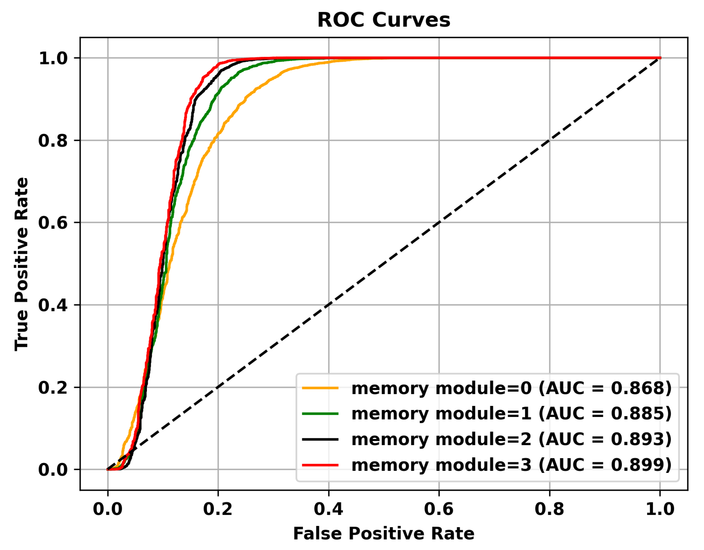
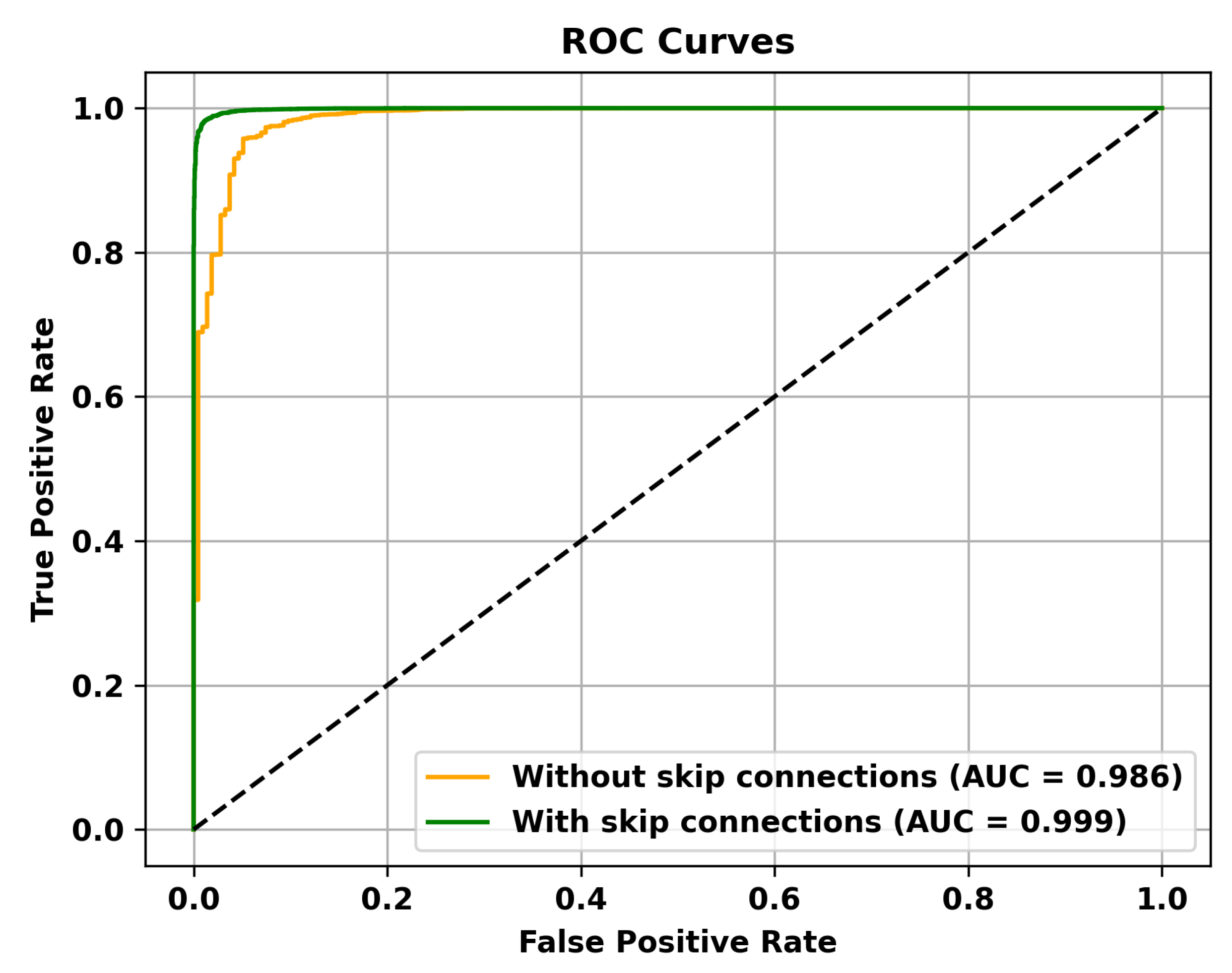
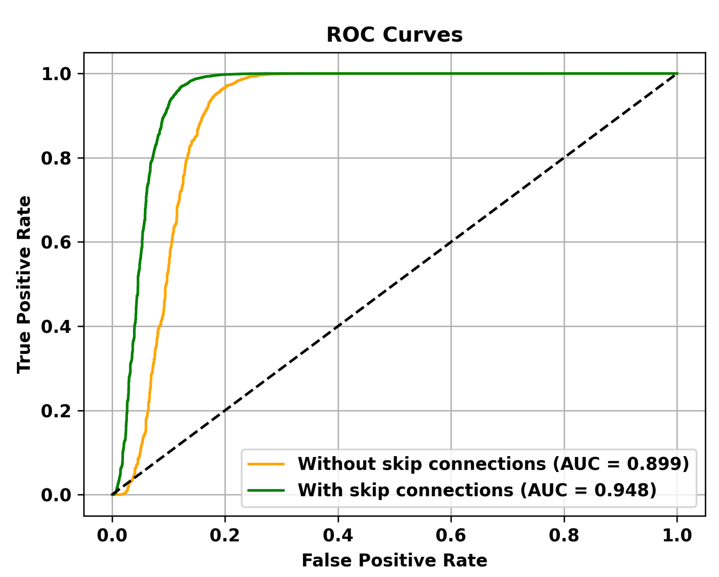
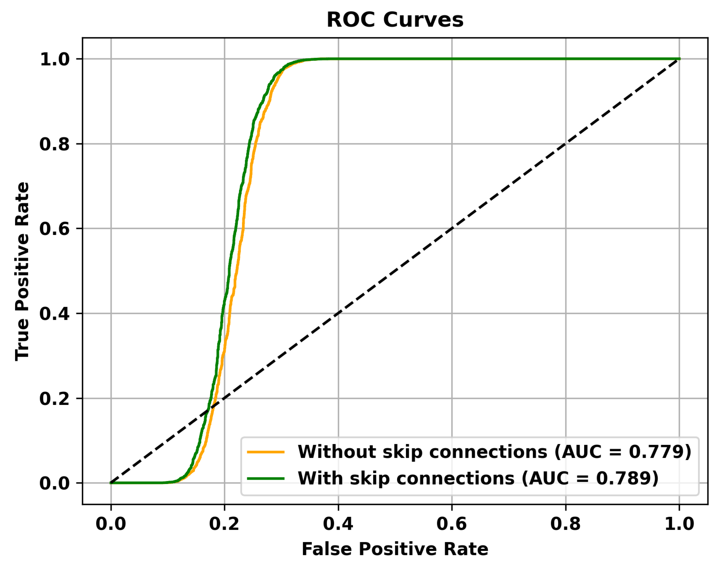
Table 5 reveals that adding multiple memory modules enhances the performance of anomaly detection, indicating that during the training process, incorporating memory modules allows for the retention of crucial features that are not masked. However, the improvement in AUC is not significant when multiple memory modules are added. This could be attributed to excessive information filtering caused by multiple memory modules, leading to network degradation and the failure to retain the most representative features. Specifically, to validate the effectiveness of the memory module, the ROC curves on three different datasets are shown in Figure 4, Figure 5 and Figure 6. To mitigate this issue, skip connections were introduced. The results presented in Table 6 illustrate an enhancement in the AUC for anomaly detection following the incorporation of skip connections. In addition, the validation of the effectiveness of skip connections on three different datasets is depicted by the ROC curves shown in Figure 7, Figure 8 and Figure 9. From the ROC curve, it is evident that the inclusion of memory modules and skip connections significantly enhances the performance of our model.
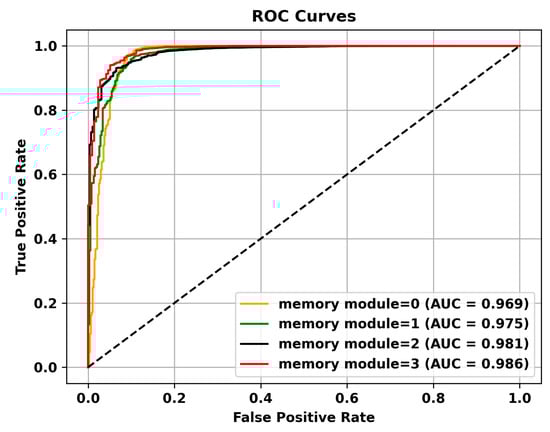
Figure 4.
The effectiveness of the memory module is validated on the UCSD Ped2 dataset.
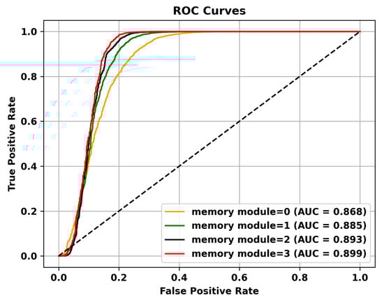
Figure 5.
The effectiveness of the memory module is validated on the Avenue dataset.
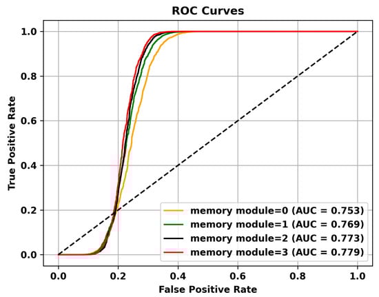
Figure 6.
The effectiveness of the memory module is validated on the Shanghai Tech dataset.
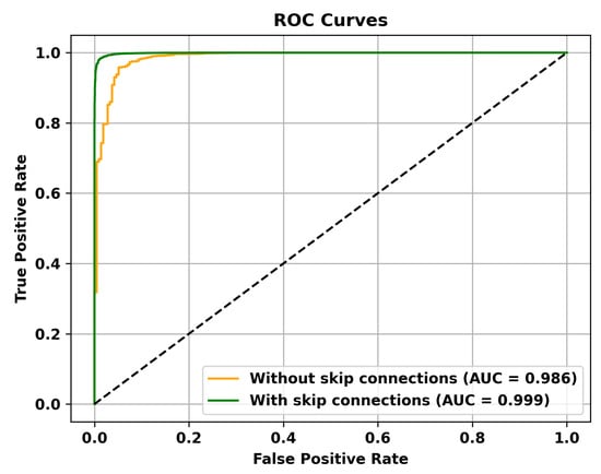
Figure 7.
The effectiveness of Skip Connections is validated on the UCSD Ped2 dataset.
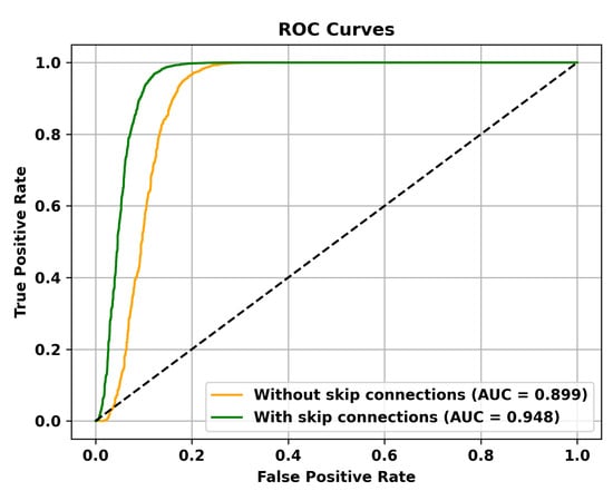
Figure 8.
The effectiveness of Skip Connections is validated on the Avenue dataset.
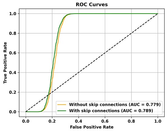
Figure 9.
The effectiveness of Skip Connections is validated on the Shanghai Tech dataset.
4.3.4. The Impact of Masking Strategy and Mask Ratios on Anomaly Score
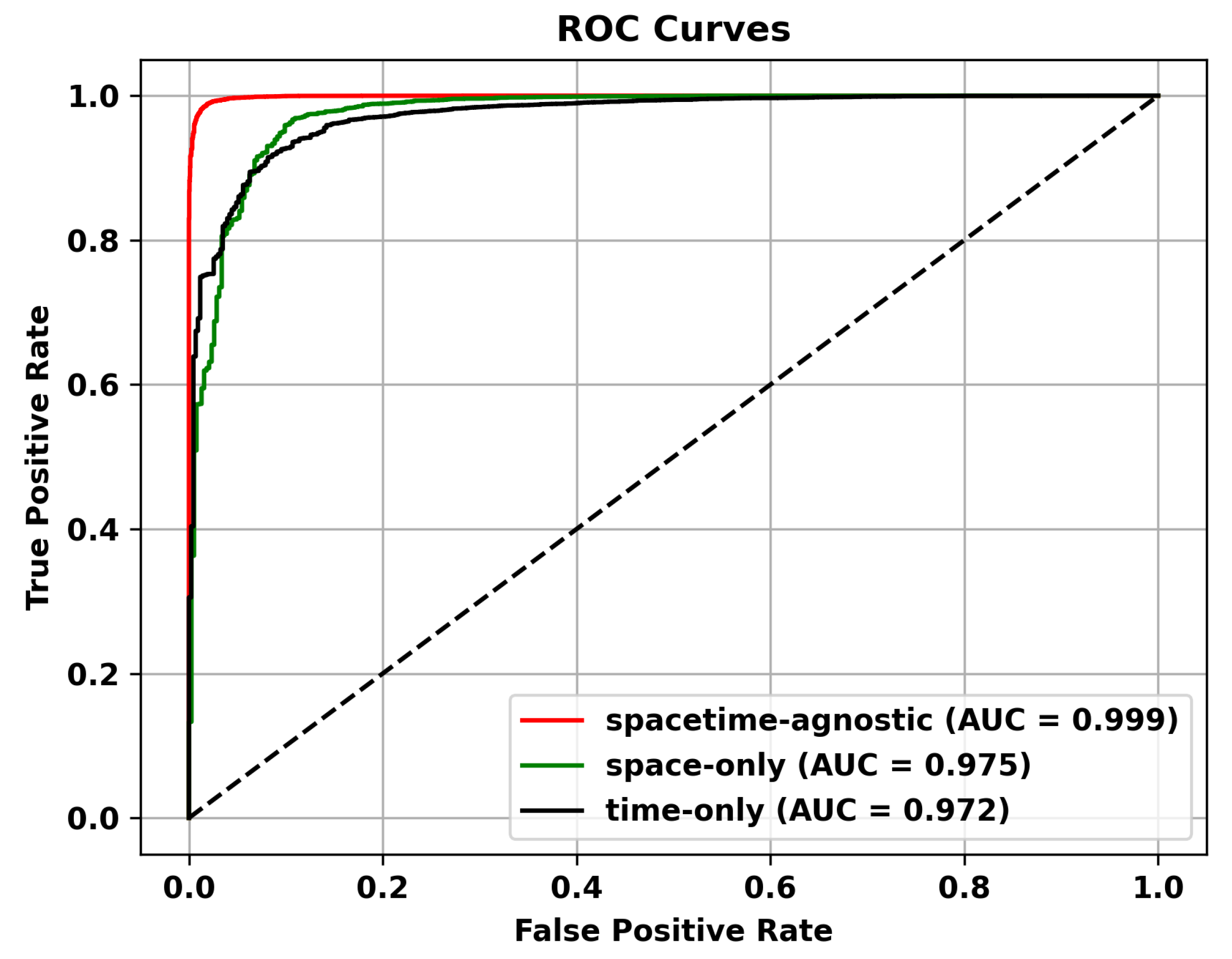
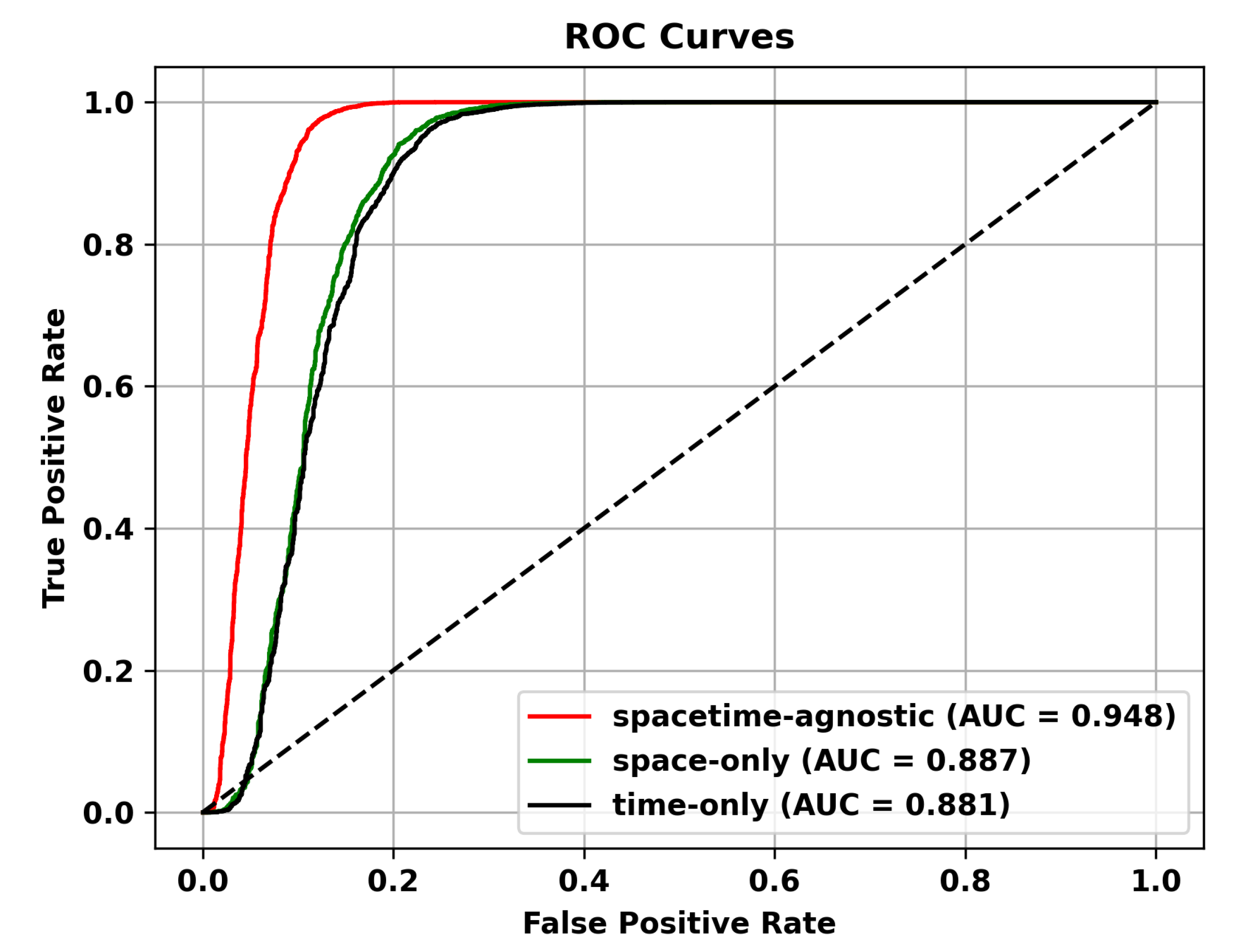
Masking Strategy. In this section, we discuss how different masking schemes affect performance. We believe that the space-only strategy, which masks only the spatial dimension, can simulate spatial occlusion, noise, or missingness, and is suitable for anomalies with spatial correlation in videos, such as moving objects or spatial shifts. However, it ignores temporal information and cannot capture temporal anomalies, such as fast-moving objects or persistent anomalies. The temporal-only strategy, which masks only the temporal dimension, can simulate temporal missingness, occlusion, or uncertainty and is suitable for temporal anomalies in videos, such as time interval or duration anomalies. However, it ignores spatial information and cannot capture spatial anomalies, such as object shape changes or spatial shifts. Given the characteristics of video anomaly detection tasks, which require capturing both temporal and spatial relationships, the optimal masking strategy should consider both spatial and temporal dimensions. The spacetime-agnostic strategy preserves complete spatial and temporal information without specific masking of either dimension. It can capture various spatiotemporal patterns and relationships and is suitable for handling diverse anomalies. Therefore, we adopt the spatiotemporal agnostic strategy. As shown in Table 7, the spatiotemporal agnostic random sampling method performs the best. Additionally, we demonstrate the superiority of the spacetime-agnostic masking strategy on different datasets through ROC curves in Figure 10, Figure 11 and Figure 12.
Table 7.
AUROC of anomaly detection under different masking strategies.
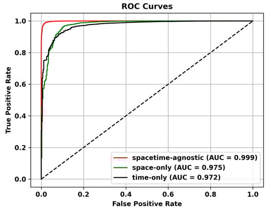
Figure 10.
ROC Curves of Different Masking Strategies on the UCSD Ped2 Dataset.

Figure 11.
ROC Curves of Different Masking Strategies on the Avenue dataset.
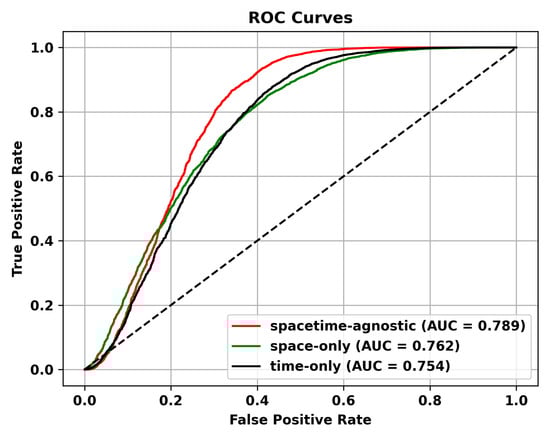
Figure 12.
ROC Curves of Different Masking Strategies on the Shanghai Tech dataset.
Mask Ratios. The influence of different mask ratios on anomaly detection performance is demonstrated in Table 8. The performance is poorest when the mask ratio is 0, demonstrating the effectiveness of masking. As the mask ratio increases, the performance consistently improves, reaching its peak at a mask ratio of 90%. However, when the mask ratio exceeds 90%, a slight decline in performance is observed. This phenomenon can be attributed to the presence of redundant information in video data, which can be effectively eliminated using the masking strategy. Consequently, the masking strategy enables the extraction of key spatiotemporal features from the videos. Nevertheless, excessively high mask ratios can lead to the obscuring of crucial information.
Table 8.
AUC of anomaly detection under different masking ratios.
4.4. Comparative Experiments
As demonstrated in Table 9, our method achieved the highest performance on the USCD Ped2 dataset. Notably, our method demonstrated a 2.0% performance gain over mainstream VAD methods on the recently utilized large-scale benchmark dataset, Avenue. However, the performance of the Shanghai Tech dataset is slightly higher than the currently prevailing state-of-the-art methods by 0.1%. This is because the Shanghai University of Science and Technology dataset contains 13 different complex environments and scenarios, such as high-density crowds, multiple movement patterns, and abnormal events. For datasets of this complexity, due to the high dependence of SMAMS performance on the selection of parameters and hyperparameters, a large amount of computational resources and time are usually required for training and evaluation. Nevertheless, our device currently does not support such large-scale operations, so in the future, we will adopt other optimization strategies to improve computational efficiency and reduce training time. In addition, comparing our method to MNAD, which also incorporates a memory module, our method exhibited slightly better performance when utilizing the memory module. This is attributed to the integration of the memory module into the ST-MAE, which enhances the model’s ability to capture long-term dependencies, incorporate contextual information, and improve the detection of abnormal patterns, therefore enhancing the effectiveness of anomaly detection.
Table 9.
Comparison of anomaly detection performance with state-of-the-art methods.
4.5. Visualization Results and Analysis
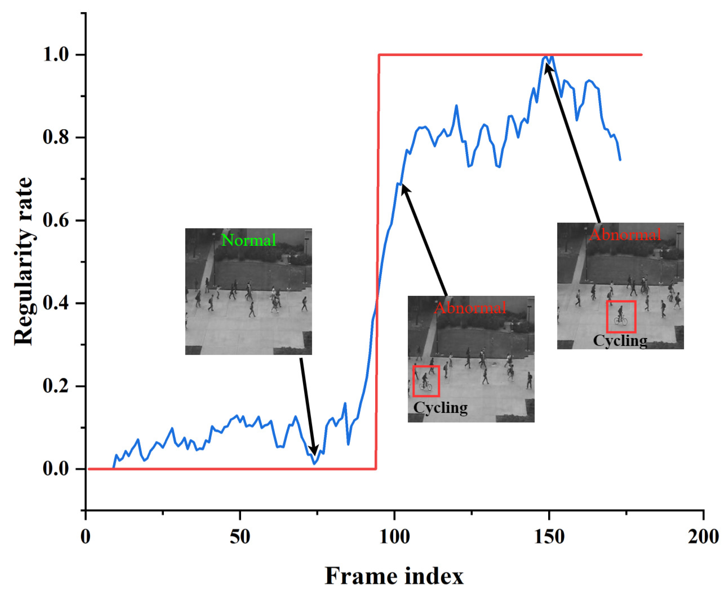
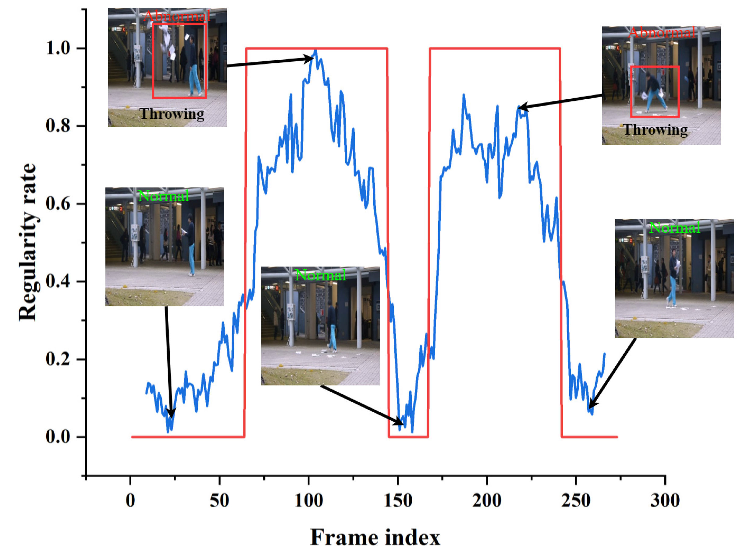
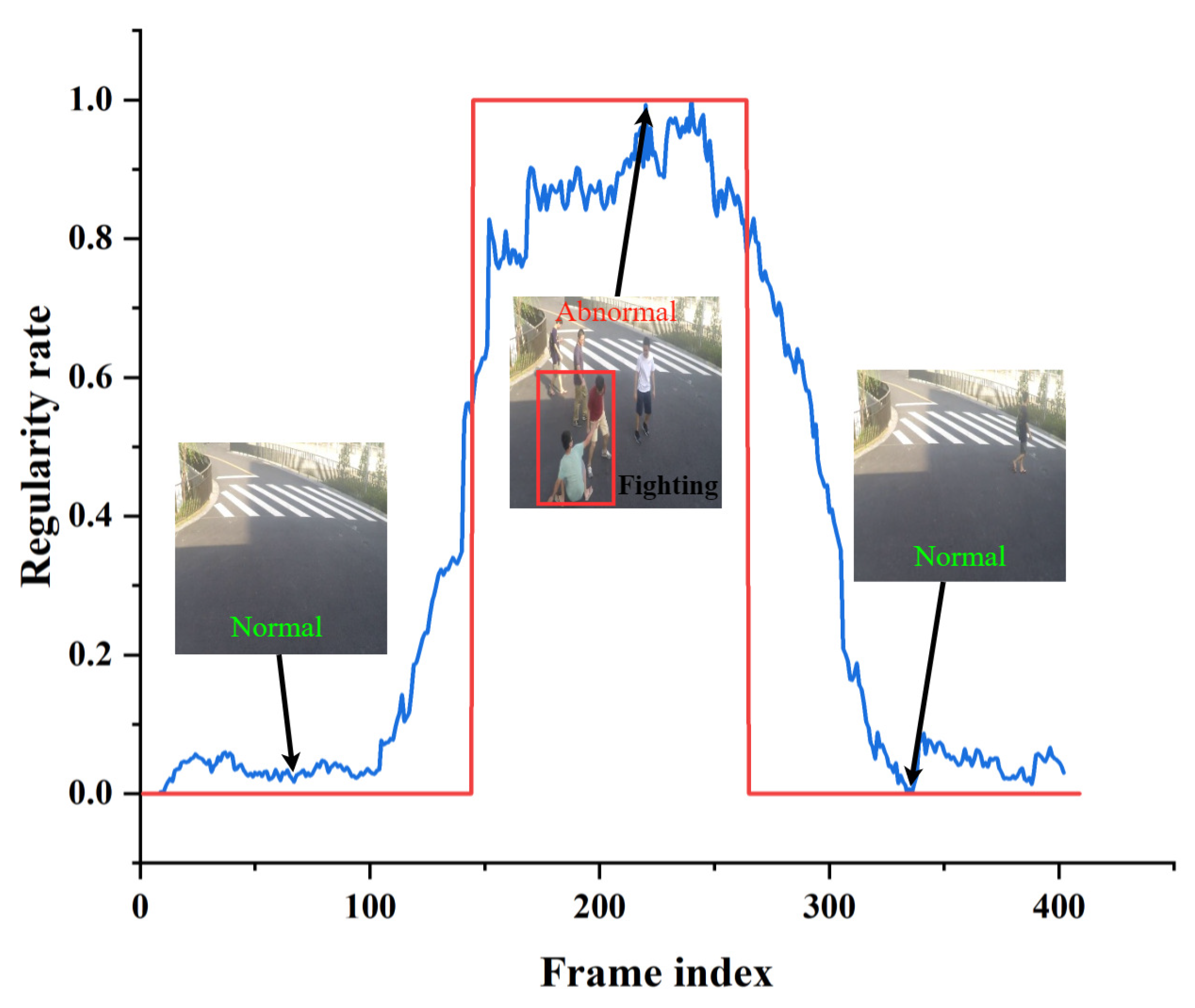
Figure 13, Figure 14 and Figure 15 shows the curve of anomaly scores and ground truth on representative test video frames from the three datasets in this study, including anomalies such as riding in a crowd, throwing objects in a public place, and fighting on a pedestrian road. The blue curve represents the anomaly score calculated by our model. At the same time, the red line segment is the ground truth, representing the true situation of the event, where 0 represents a normal frame, and 1 represents an abnormal frame. The figure shows that the ground truth and anomaly scores have similar changes, indicating that our model can respond correctly to normal and abnormal events. Specifically, when an abnormal object suddenly appears, the anomaly score curve sharply increases, and when an abnormal event occurs, the curve remains at a high level. The curve quickly drops to a low level when the abnormal event disappears. The experimental results provide validation for the effectiveness of the proposed model in accurately identifying abnormal events in surveillance video data. The model demonstrates robust and accurate detection performance across a range of different scenarios and various types of abnormal events. Through testing on three different datasets, we found that our model can adapt well to different scenarios and maintain high accuracy in anomaly detection. Our model has proven effective in distinguishing between normal and abnormal frames, making it highly applicable in practical scenarios.
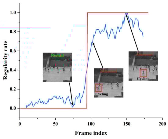
Figure 13.
Typical test video from the UCSD Ped2 dataset. The blue curve represents the anomaly score calculated by our model. The red line segment is the ground truth.

Figure 14.
Typical test video from the Avenue dataset. The blue curve represents the anomaly score calculated by our model. The red line segment is the ground truth.

Figure 15.
Typical test video from the ShanghaiTech dataset. The blue curve represents the anomaly score calculated by our model. The red line segment is the ground truth.
5. Conclusions and Future Work
This paper proposes a VAD method based on ST-MAE and memory modules. First, we extract spatiotemporal cubes by capturing appearance and motion clues for precise and comprehensive video event extraction. Second, we perform random masked foreground patching on the spatiotemporal cubes, extract feature representations of the unmasked patched regions using a pre-trained ViT model, and input them into the decoder for predicting the masked patches to learn the high-level semantics of video events. Finally, we design multiple memory modules based on the ST-MAE to store unmasked video patch features of different feature layers and add skip connections to compensate for performance degradation caused by information loss due to the memory modules to better distinguish between normal and abnormal videos. Experiments on three public datasets show that the proposed method is effective and outperforms state-of-the-art approaches in terms of performance. Ablation experiments demonstrate the contributions of each model component to excellent performance. In addition, the visualization of experimental results further demonstrates the effectiveness and robustness of the proposed method.
When dealing with complex anomaly scenes in the real world, we recognize the need for optimization strategies to enhance computational efficiency and reduce training time. Given the high sensitivity of SMAMS performance to parameter and hyperparameter selection, we acknowledge the challenges posed by the requirement of extensive computational resources and time for training and evaluation on complex datasets. To address these challenges, we aim to investigate optimized techniques that are specifically designed for complex scenarios in the future.
Author Contributions
Writing—original draft preparation, B.Y.; writing—review and editing, Y.F.; funding acquisition, O.Y. All authors have read and agreed to the published version of the manuscript.
Funding
This research was funded by the Chinese Postdoctoral Science Foundation under Grant No. 2020M673446.
Data Availability Statement
The datasets generated during and/or analyzed during the current study are available from the corresponding author upon reasonable request.
Conflicts of Interest
The authors declare no conflict of interest.
References
- Cong, Y.; Yuan, J.; Liu, J. Sparse reconstruction cost for abnormal event detection. In Proceedings of the CVPR 2011, Colorado Springs, CO, USA, 20–25 June 2021; IEEE: Piscataway, NJ, USA, 2011; pp. 3449–3456. [Google Scholar]
- Mahadevan, V.; Li, W.; Bhalodia, V.; Vasconcelos, N. Anomaly detection in crowded scenes. In Proceedings of the 2010 IEEE Computer Society Conference on Computer Vision and Pattern Recognition, San Francisco, CA, USA, 13–18 June 2010; IEEE: Piscataway, NJ, USA, 2010; pp. 1975–1981. [Google Scholar]
- Gong, D.; Liu, L.; Le, V.; Saha, B.; Mansour, M.R.; Venkatesh, S.; Hengel, A.v.d. Memorizing normality to detect anomaly: Memory-augmented deep autoencoder for unsupervised anomaly detection. In Proceedings of the IEEE/CVF International Conference on Computer Vision, Seoul, Republic of Korea, 27 October–2 November 2019; pp. 1705–1714. [Google Scholar]
- Le, V.T.; Kim, Y.G. Attention-based residual autoencoder for video anomaly detection. Appl. Intell. 2023, 53, 3240–3254. [Google Scholar] [CrossRef]
- Wei, H.; Li, K.; Li, H.; Lyu, Y.; Hu, X. Detecting video anomaly with a stacked convolutional LSTM framework. In Proceedings of the Computer Vision Systems: 12th International Conference, ICVS 2019, Thessaloniki, Greece, 23–25 September 2019; Proceedings 12. Springer: Berlin/Heidelberg, Germany, 2019; pp. 330–342. [Google Scholar]
- Larsen, A.B.L.; Sønderby, S.K.; Larochelle, H.; Winther, O. Autoencoding beyond pixels using a learned similarity metric. In Proceedings of the International Conference on Machine Learning, New York, NY, USA, 20–22 June 2016; pp. 1558–1566. [Google Scholar]
- Feng, X.; Song, D.; Chen, Y.; Chen, Z.; Ni, J.; Chen, H. Convolutional transformer based dual discriminator generative adversarial networks for video anomaly detection. In Proceedings of the 29th ACM International Conference on Multimedia, Virtual, 20–24 October 2021. [Google Scholar]
- Liu, W.; Luo, W.; Lian, D.; Gao, S. Future frame prediction for anomaly detection—A new baseline. In Proceedings of the IEEE Conference on Computer Vision and Pattern Recognition, Salt Lake City, UT, USA, 18–23 June 2018; pp. 6536–6545. [Google Scholar]
- Lu, Y.; Kumar, K.M.; Shahabeddin Nabavi, S.; Wang, Y. Future frame prediction using convolutional VRNN for anomaly detection. In Proceedings of the 2019 16th IEEE International Conference on Advanced Video and Signal Based Surveillance (AVSS), Taipei, Taiwan, 18–21 September 2019; IEEE: Piscataway, NJ, USA, 2019; pp. 1–8. [Google Scholar]
- Tang, Y.; Zhao, L.; Zhang, S.; Gong, C.; Li, G.; Yang, J. Integrating prediction and reconstruction for anomaly detection. Pattern Recognit. Lett. 2020, 129, 123–130. [Google Scholar] [CrossRef]
- Zhao, Y.; Deng, B.; Shen, C.; Liu, Y.; Lu, H.; Hua, X.S. Spatio-temporal autoencoder for video anomaly detection. In Proceedings of the 25th ACM International Conference on Multimedia, Mountain View, CA, USA, 23–27 October 2017; pp. 1933–1941. [Google Scholar]
- Ye, M.; Peng, X.; Gan, W.; Wu, W.; Qiao, Y. Anopcn: Video anomaly detection via deep predictive coding network. In Proceedings of the 27th ACM International Conference on Multimedia, Nice, France, 21–25 October 2019; pp. 1805–1813. [Google Scholar]
- Fan, Y.; Wen, G.; Li, D.; Qiu, S.; Levine, M.D.; Xiao, F. Video anomaly detection and localization via gaussian mixture fully convolutional variational autoencoder. Comput. Vis. Image Underst. 2020, 195, 102920. [Google Scholar] [CrossRef]
- Deepak, K.; Chandrakala, S.; Mohan, C.K. Residual spatiotemporal autoencoder for unsupervised video anomaly detection. Signal Image Video Process. 2021, 15, 215–222. [Google Scholar] [CrossRef]
- Kommanduri, R.; Ghorai, M. Bi-READ: Bi-Residual AutoEncoder based feature enhancement for video anomaly detection. J. Vis. Commun. Image Represent. 2023, 95, 103860. [Google Scholar] [CrossRef]
- Joshi, K.V.; Patel, N.M. Anomaly Detection in Surveillance Scenes Using Autoencoders. SN Comput. Sci. 2023, 4, 804. [Google Scholar] [CrossRef]
- Waseem, F.; Martinez, R.P.; Wu, C. Visual anomaly detection in video by variational autoencoder. arXiv 2022, arXiv:2203.03872. [Google Scholar]
- Li, N.; Chang, F.; Liu, C. Spatial-temporal cascade autoencoder for video anomaly detection in crowded scenes. IEEE Trans. Multimed. 2020, 23, 203–215. [Google Scholar] [CrossRef]
- Li, T.; Chen, X.; Zhu, F.; Zhang, Z.; Yan, H. Two-stream deep spatial-temporal auto-encoder for surveillance video abnormal event detection. Neurocomputing 2021, 439, 256–270. [Google Scholar] [CrossRef]
- Liu, Y.; Liu, J.; Zhao, M.; Yang, D.; Zhu, X.; Song, L. Learning Appearance-Motion Normality for Video Anomaly Detection. In Proceedings of the 2022 IEEE International Conference on Multimedia and Expo (ICME), Taipei, Taiwan, 18–22 July 2022; IEEE: Piscataway, NJ, USA, 2022; pp. 1–6. [Google Scholar]
- Wang, X.; Che, Z.; Jiang, B.; Xiao, N.; Yang, K.; Tang, J.; Ye, J.; Wang, J.; Qi, Q. Robust unsupervised video anomaly detection by multipath frame prediction. IEEE Trans. Neural Netw. Learn. Syst. 2021, 33, 2301–2312. [Google Scholar] [CrossRef] [PubMed]
- Zhao, M.; Liu, Y.; Liu, J.; Zeng, X. Exploiting Spatial-temporal Correlations for Video Anomaly Detection. In Proceedings of the 2022 26th International Conference on Pattern Recognition (ICPR), Montreal, QC, Canada, 21–25 August 2022; IEEE: Piscataway, NJ, USA, 2022; pp. 1727–1733. [Google Scholar]
- Xu, H.; Liu, W.; Xing, W.; Wei, X. Motion-aware future frame prediction for video anomaly detection based on saliency perception. Signal Image Video Process. 2022, 16, 2121–2129. [Google Scholar] [CrossRef]
- Baradaran, M.; Bergevin, R. Future Video Prediction from a Single Frame for Video Anomaly Detection. In Proceedings of the International Symposium on Visual Computing, Lake Tahoe, NV, USA, 16–18 October 2023; Springer: Berlin/Heidelberg, Germany, 2023; pp. 472–486. [Google Scholar]
- Deng, H.; Zhang, Z.; Zou, S.; Li, X. Bi-Directional Frame Interpolation for Unsupervised Video Anomaly Detection. In Proceedings of the IEEE/CVF Winter Conference on Applications of Computer Vision, Waikoloa, HI, USA, 2–7 January 2023; pp. 2634–2643. [Google Scholar]
- Cheng, K.; Zeng, X.; Liu, Y.; Zhao, M.; Pang, C.; Hu, X. Spatial-Temporal Graph Convolutional Network Boosted Flow-Frame Prediction For Video Anomaly Detection. In Proceedings of the ICASSP 2023–2023 IEEE International Conference on Acoustics, Speech and Signal Processing (ICASSP), Rhodes Island, Greece, 4–10 June 2023; IEEE: Piscataway, NJ, USA, 2023; pp. 1–5. [Google Scholar]
- Li, C.; Li, H.; Zhang, G. Future frame prediction based on generative assistant discriminative network for anomaly detection. Appl. Intell. 2023, 53, 542–559. [Google Scholar] [CrossRef]
- Zhang, Q.; Feng, G.; Wu, H. Surveillance video anomaly detection via non-local U-Net frame prediction. Multimed. Tools Appl. 2022, 81, 27073–27088. [Google Scholar] [CrossRef]
- Graves, A.; Wayne, G.; Reynolds, M.; Harley, T.; Danihelka, I.; Grabska-Barwińska, A.; Colmenarejo, S.G.; Grefenstette, E.; Ramalho, T.; Agapiou, J.; et al. Hybrid computing using a neural network with dynamic external memory. Nature 2016, 538, 471–476. [Google Scholar] [CrossRef] [PubMed]
- Park, H.; Noh, J.; Ham, B. Learning memory-guided normality for anomaly detection. In Proceedings of the IEEE/CVF Conference on Computer Vision and Pattern Recognition, Seattle, WA, USA, 13–19 June 2020; pp. 14372–14381. [Google Scholar]
- Fernando, T.; Denman, S.; Ahmedt-Aristizabal, D.; Sridharan, S.; Laurens, K.R.; Johnston, P.; Fookes, C. Neural memory plasticity for medical anomaly detection. Neural Netw. 2020, 127, 67–81. [Google Scholar] [CrossRef] [PubMed]
- Yu, L.; Qiao, B.; Zhang, H.; Yu, J.; He, X. LTST: Long-term segmentation tracker with memory attention network. Image Vis. Comput. 2022, 119, 104374. [Google Scholar] [CrossRef]
- Ravanbakhsh, M.; Nabi, M.; Sangineto, E.; Marcenaro, L.; Regazzoni, C.; Sebe, N. Abnormal event detection in videos using generative adversarial nets. In Proceedings of the 2017 IEEE International Conference on Image Processing (ICIP), Beijing, China, 17–20 September 2017; IEEE: Piscataway, NJ, USA, 2017; pp. 1577–1581. [Google Scholar]
- Sabokrou, M.; Khalooei, M.; Fathy, M.; Adeli, E. Adversarially learned one-class classifier for novelty detection. In Proceedings of the IEEE Conference on Computer Vision and Pattern Recognition, Salt Lake City, UT, USA, 18–23 June 2018; pp. 3379–3388. [Google Scholar]
- Hasan, M.; Choi, J.; Neumann, J.; Roy-Chowdhury, A.K.; Davis, L.S. Learning temporal regularity in video sequences. In Proceedings of the IEEE Conference on Computer Vision and Pattern Recognition, Las Vegas, NV, USA, 27–30 June 2016; pp. 733–742. [Google Scholar]
- Liu, Z.; Nie, Y.; Long, C.; Zhang, Q.; Li, G. A hybrid video anomaly detection framework via memory-augmented flow reconstruction and flow-guided frame prediction. In Proceedings of the IEEE/CVF International Conference on computer Vision, Montreal, QC, Canada, 10–17 October 2021; pp. 13588–13597. [Google Scholar]
- Lu, C.; Shi, J.; Jia, J. Abnormal event detection at 150 fps in MATLAB. In Proceedings of the IEEE International Conference on Computer Vision, Sydney, NSW, Australia, 1–8 December 2013; pp. 2720–2727. [Google Scholar]
- Luo, W.; Liu, W.; Gao, S. A revisit of sparse coding based anomaly detection in stacked rnn framework. In Proceedings of the IEEE International Conference on Computer Vision, Venice, Italy, 22–29 October 2017; pp. 341–349. [Google Scholar]
- Fang, Z.; Liang, J.; Zhou, J.T.; Xiao, Y.; Yang, F. Anomaly detection with bidirectional consistency in videos. IEEE Trans. Neural Netw. Learn. Syst. 2020, 33, 1079–1092. [Google Scholar] [CrossRef] [PubMed]
- Liu, Y.; Li, S.; Liu, J.; Yang, H.; Zhao, M.; Zeng, X.; Ni, W.; Song, L. Learning Attention Augmented Spatial-temporal Normality for Video Anomaly Detection. In Proceedings of the 2021 3rd International Symposium on Smart and Healthy Cities (ISHC), Toronto, ON, Canada, 28–29 December 2021; IEEE: Piscataway, NJ, USA, 2021; pp. 137–144. [Google Scholar]
- Chang, Y.; Tu, Z.; Xie, W.; Luo, B.; Zhang, S.; Sui, H.; Yuan, J. Video anomaly detection with spatio-temporal dissociation. Pattern Recognit. 2022, 122, 108213. [Google Scholar] [CrossRef]
- Hirschorn, O.; Avidan, S. Normalizing flows for human pose anomaly detection. In Proceedings of the IEEE/CVF International Conference on Computer Vision, Paris, France, 2–6 October 2023; pp. 13545–13554. [Google Scholar]


Disclaimer/Publisher’s Note: The statements, opinions and data contained in all publications are solely those of the individual author(s) and contributor(s) and not of MDPI and/or the editor(s). MDPI and/or the editor(s) disclaim responsibility for any injury to people or property resulting from any ideas, methods, instructions or products referred to in the content. |
© 2024 by the authors. Licensee MDPI, Basel, Switzerland. This article is an open access article distributed under the terms and conditions of the Creative Commons Attribution (CC BY) license (https://creativecommons.org/licenses/by/4.0/).