Three-Dimensional-Consistent Scene Inpainting via Uncertainty-Aware Neural Radiance Field

Abstract

3D (Three-Dimensional) scene inpainting aims to remove objects from scenes and generate visually plausible regions to fill the hollows. Leveraging the foundation of NeRF (Neural Radiance Field), considerable advancements have been achieved in the realm of 3D scene inpainting. However, prevalent issues persist: primarily, the presence of inconsistent 3D details across different viewpoints and occlusion losses of real background details in inpainted regions. This paper presents a NeRF-based inpainting approach using uncertainty estimation that formulates mask and uncertainty branches for consistency enhancement. In the initial training, the mask branch learns a 3D-consistent representation from inaccurate input masks, and after background rendering, the background regions can be fully exposed to the views. The uncertainty branch learns the visibility of spatial points by modeling them as Gaussian distributions, generating variances to identify regions to be inpainted. During the inpainting training phase, the uncertainty branch measures 3D consistency in the inpainted views and calculates the confidence from the variance as dynamic weights, which are used to balance the color and adversarial losses to achieve 3D-consistent inpainting with both the structure and texture. The results were evaluated on datasets such as Spin-NeRF and NeRF-Object-Removal. The proposed approach outperformed the baselines in inpainting metrics of LPIPS and FID, and preserved more spatial details from real backgrounds in multi-scene settings, thus achieving 3D-consistent restoration.

1. Introduction

A NeRF (Neural Radiance Field) [1] is a deep learning-based 3D reconstruction method that was proposed by Mildenhall et al. in 2020. Employing multi-layer perceptron networks in conjunction with ray casting [2], a NeRF adeptly learns the color information of points in 3D scenes, thereby enabling the generation of high-quality 3D scenes from a small number of 2D (Two-Dimensional) image samples. In recent years, research into NeRFs has advanced significantly. Numerous endeavors have aimed at augmenting their performance and expanding their applicability via, for instance, improving the training speed [3,4,5], reducing view input requirements [6,7], facilitating scene editing [8,9], and extending their functionality to dynamic scenes [10,11]. Driven by the needs of practical applications, NeRf editing methods [9,12,13,14,15,16,17,18,19] have emerged as a focal point of current research. Among these methods, NeRF inpainting [17,18,19] holds particular prominence as a widely applicable editing technique with considerable potential. It involves removing specified objects from NeRF scenes and inpainting the resultant hollow regions. Unlike well-established 2D inpainting methods, NeRF inpainting necessitates additional 3D consistency. Nevertheless, prevailing approaches exhibit certain limitations in preserving real background details and inpainting visually plausible structure and texture. The primary objective of this paper was to improve existing NeRF inpainting methods by maximizing the preservation of real details and achieving superior inpainting outcomes.

Existing 2D image inpainting methods [20,21,22,23,24,25,26,27,28,29,30] have demonstrated impressive capabilities to restore and reconstruct specified regions in complex images while ensuring high fidelity. Some of them [24,25] utilize image generation networks as a foundation for image inpainting, while others [26,27,28,29] improve the inpainting networks by leveraging image characteristics, such as the frequency domain and structure. However, most of the above-mentioned methods use 2D convolution as the basic module and cannot be directly applied to 3D scenes with multiple views. Furthermore, directly removing or inpainting objects in NeRFs is challenging owing to the intricate association between network parameters and the geometric appearance of the scene. Consequently, retraining NeRFs using inpainted views as priors has become a mainstream solution. Shen et al. [17] pioneered a comprehensive two-stage architecture tailored for NeRF inpainting. In their approach, the initial training phase involves reconstructing the original scene using a NeRF, thus producing color and depth view sequences. These view sequences, coupled with masks of the target object, are subsequently input into a 2D inpainting model. During the inpainting training phase, RGB (Red Green Blue) and depth images generated by the 2D model serve as priors for a new NeRF to obtain an inpainting scene. This method relies solely on a single inpainted view as supervision for the repaired region, which makes it challenging to model view-dependent effects. Consequently, the inpainted region becomes blurry when rendering from other viewpoints. Addressing this limitation, Mirzaei et al. [18] used all inpainted views as supervision, employing perceptual loss to train inpainted regions to avoid blurring issues arising from the direct utilization of color loss under 3D inconsistent multi-view priors. Additionally, they utilized a depth map to establish pixel correspondences between different views [31], enabling the acquisition of color information from another view to fill in the current view. This strategy facilitates the incorporation of real background information to complete the restored region. However, directly using color from other viewpoints ignores the view-dependent effects, and inaccuracies in the NeRF introduce errors in the filling process. Moreover, an exclusive reliance on perceptual loss can lead to texture-based artifacts in the inpainted regions. In response to these challenges, Weder et al. [19] proposed a strategy aiming to address the 3D-consistent issue by learning the confidence of each view and progressively removing low-confidence images from the training set during the training process. The difficulty, however, lies in the fact that inaccurate masks cause the loss of real background information, and for scenes with complex textures, this method remains susceptible to artifact generation.

Recent advancements in NeRF inpainting highlight two primary challenges that necessitate attention. Firstly, most existing methods do not introduce or introduce inaccurate 3D background information. Unlike 2D images where one pixel corresponds to an entire camera ray, 3D scenes present a complexity wherein some camera rays may traverse both the foreground and background. In such cases, simply disregarding the foreground region during rendering can yield background views. Therefore, the background region completely occluded by the target object in the training set represents the actual area requiring inpainting. Secondly, current methods have yet to achieve 3D-consistent inpainting results while simultaneously considering texture and structure. The intermediate results obtained by a 2D model for the same scene may not be consistent. Training a NeRF using 2D results with simple color loss tends to induce blurring issues, while relying solely on a perceptual loss will lead to excessive texture artifacts. Hence, integrating the two types of losses to improve inpainting performance constitutes a promising avenue worthy of exploration.

In this paper, we propose a novel architecture for removing selected objects based on a NeRF and subsequently inpainting the resultant hollow regions. Our model integrates a mask branch and an uncertainty branch to overcome the issue of losing real 3D background information. During the initial training phase, the mask branch captures detailed segmentation masks of the target object to achieve background rendering and expose more background information. By fully utilizing the generalization capability of the NeRF, it contributes to acquiring 3D-consistent annotations for the target object. In the uncertainty branch, each point in the 3D scene is modeled as a Gaussian distribution, and the visibility of the spatial points is learned in an unsupervised manner by minimizing the negative log-likelihood. After background rendering, regions with a high variance are identified as requiring inpainting. Then, optimized masks are input to a pre-trained 2D inpainting model to obtain prior outputs for subsequent training. Throughout the inpainting training, we employ a dynamic weight loss to address the imbalance between structure and texture of the inpainting NeRF. Moreover, the same loss as in the first stage is utilized to train the uncertainty branch, incorporating the output variance as a measure of 3D consistency in 2D priors, resulting in improved outcomes.

The contributions of this paper are as follows:

(1)

The mask branch is introduced based on the radiance field. By leveraging the strong generalizability of the radiance field, it is possible to train 3D-consistent segmentation results from mask information that may contain errors. Using this branch for rendering background views enables the preservation of more real background information during the 2D inpainting process;

(2)

The uncertainty branch based on the normal distribution is innovatively used in the NeRF inpainting task. Every spatial point is modeled as a Gaussian distribution, and the uncertainty branch outputs the variance. Through minimizing the negative log-likelihood loss, it is possible to learn the visibility of spatial points in an unsupervised manner. This branch aids in identifying regions in the background views that require inpainting, thereby optimizing the mask used for 2D manipulation;

(3)

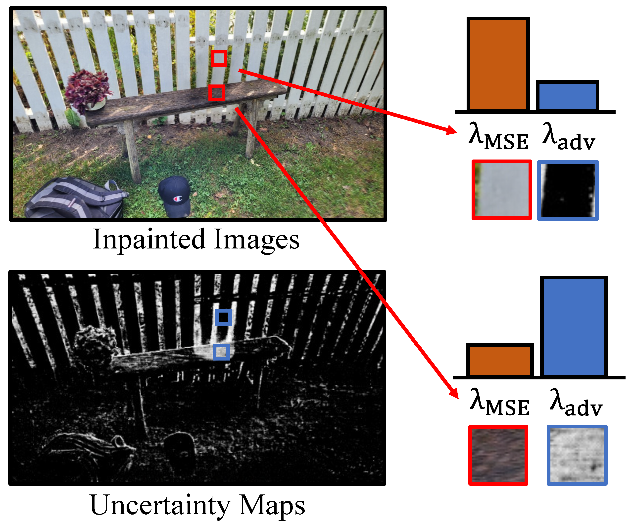
A new dynamic weight training strategy is proposed to further enhance the optimization effect by utilizing the uncertainty branch. During the inpainting training stage, the uncertainty branch is adopted to measure the 3D consistency of 2D inpainted views. Based on the variance output from this branch, the confidence of the sampled ray’s color is calculated and used as dynamic weights for both the color loss and adversarial loss. This approach achieves a balance between structure and texture in the inpainted regions of 3D scenes.

2. Related Work

2.1. Image Inpainting

Image inpainting is a digital image processing technique that aims to remove unwanted or damaged regions from an image and replace them with appropriate content. Traditional methods for image inpainting predominantly rely on statistical information and geometric structures of images, broadly categorized into diffusion-based [20,21] and patch-based methods [22,23]. However, they have high computational complexity and low fidelity.

The integration of deep learning into computer vision has sparked massive scholarly interest in image inpainting methods based on deep learning. Recent research focuses on leveraging generative network advancements to achieve more realistic image inpainting effects. Wang et al. [24] utilized prior information from pre-trained StyleGAN [32] to perform image inpainting using GAN (Generative Adversarial Network) inversion, while Liu et al. [25] opted to inject initial image and mask information into the generation process. The subsequent advent of the DDPM (Denoising Diffusion Probability Model) [33] also provided new impetus for image inpainting. RePaint [30] used a pre-trained unconditional DDPM as a generative prior model. Other methods attempt to mine information beyond image color and use it to further optimize the inpainting process. The work of Cao et al. [26] and their improved method [27] repaired the multi-scale structure as a guide for subsequent color inpainting to achieve an improved overall generated structure. Domain transformation operations can also yield good results. Yu et al. [28] used wavelet decomposition to handle conflicts between different frequencies in images, while Suvorov et al. [29] combined Fourier transformation to enhance the receptive field of convolution and improve the ability to repair large areas.

These approaches are only designed for 2D image scenarios. This implies that when they inpaint different views of the same scene, inconsistent results will be obtained. However, the individual image inpainted result is visually good, so we consider the 2D model outputs as priors. Thus, the contribution of this paper lies in its applicability to any 3D scene represented by a NeRF, enabling the attainment of 3D-consistent inpainting results.

2.2. NeRF Edit

NeRFs, an implicit 3D scene representation based on neural networks, have garnered growing attention in recent years. Rapid advancements and improvements have been made regarding training speed [3,4,5], geometric quality [34,35], and dynamic representation [10,11]. Moreover, NeRF scene editing has also become a hot research topic, emphasizing the editing of texture and geometry. Specifically, texture editing involves using pre-trained 2D models as priors [12], using style loss as guidance [13], and performing traditional color modification using color palettes [14]. Geometric information editing predominantly revolves around learned standard spatial representations and additional deformation fields [15]. Furthermore, research related to interactive NeRF editing has focused more on interactive target selection [16] or semantic editing [9].

Within the realm of 3D scene editing, NeRF inpainting has made notable strides in recent research endeavors [17,18,19]. The NeRF-In [17] approach proposed the NeRF inpainting architecture for the first time, using a video segmentation model on the sequence of images rendered by a NeRF to select objects to be removed. It utilized an image inpainting model for object removal at the 2D level, treating its outputs as priors, alongside leveraging the inpainted depth map for geometric supervision. The Spin-NeRF [18] approach improved upon this approach by using SemanticNerf [36] to optimize the mask of the target object and added a perception loss to obtain better results. Weder et al. [19] evaluated the consistency of each inpainted image during training to optimize subsequent training.

Nevertheless, some of these methods overlook the 3D characteristic of the scenes and directly mark the object masks in a 2D image, resulting in the loss of some real background information. Others struggle to strike a balance between structure and texture, leading to blurring or other artifacts. Our method was built upon the NeRF-In approach with two-stage training. In the first stage, background information is preserved extensively, while in the second stage, we improve the repair results through a unique dynamic weight loss.

2.3. Uncertainty Estimation

Uncertainty estimation refers to estimating the reliability of network outputs. To achieve uncertainty in the network, Bayesian neural networks [37,38] set the weights as a probability distribution, optimizing the distribution’s parameters during the optimization process. One common approach is to use variational inference with Dropout layers and input the same data multiple times [39]. The posterior distribution is extensively adopted for uncertainty estimation.

Uncertainty estimation in a NeRF is mainly used to learn the uncertainty of spatial point attributes, like the color or density, caused by insufficient or inconsistent training views. These methods utilize the framework proposed by Kendall et al. [40] designed for uncertainty estimation in the field of computer vision to quantitatively assess the reliability of a NeRF’s outputs or enhance generalization performance. Most methods model spatial points as parameterized distributions to estimate uncertainty. The work on NeRF-w in [41] used uncertainty estimation to handle transient scene information present in outdoor images, while the ActiveNeRF [42] method employs it for active learning of sample selection in few-shot scenarios. The DS-NeRF [43] approach extends uncertainty estimation in color to the geometric level of the radiance field, providing depth supervision with some freedom, thereby achieving better generalization ability with sparse supervision.

This paper aligns with the above methods in modeling parameterized distributions, but it stands out as the pioneer in applying uncertainty estimation to the NeRF inpainting task. In our approach, uncertainty is used to represent the visibility of points and the consistency of 2D inpainted views, which are achieved through minimizing the negative log-likelihood loss. In this approach, we are able to apply different weights to loss functions for structure and texture, achieving a balanced effect.

3. Method

This study introduces UC-NeRF, a novel architecture designed for removing specified objects from the NeRF and subsequently inpainting invisible regions. The aim of the NeRF was to reconstruct a 3D scene from given sets of views $\mathcal{I}={\left\{I_i\right\}}_{i=1}^n$, and their corresponding poses $\mathcal{P}={\left\{P_i\right\}}_{i=1}^n$ and camera intrinsic K. On this basis, an initial mask $M_i$ for a given view $I_i$ was further added to the inputs of NeRF inpainting to specify the object to be removed. Compared to existing methods, the UC-NeRF approach excelled in recovering the complete scene geometry and color information, ensuring both visual plausibility and 3D consistency within the inpainted area.

For NeRF implementation, TensoRF [5] was used as the baseline due to its faster convergence speed. We first introduced two branches: the mask branch ${\mathcal{G}}_m$ and the uncertainty branch ${\mathcal{G}}_{\beta }$ (refer to Section 3.1). These two branches could enhance the representation capabilities. The input views and masks were then optimized by mask optimization (refer to Section 3.2) to capture as much background information as possible throughout the dataset. Subsequently, the optimized images were re-drawn using an off-the-shelf image inpainting model. When training the inpainted NeRF, the output of the uncertainty branch was used to dynamically balance the weights of the color loss and adversarial loss to achieve better 3D-consistent results (refer to Section 3.3). In summary, our method could maximize the utilization of 3D scene information in the entire dataset to minimize inconsistent view areas caused by the 2D model, thereby achieving more accurate object removal and scene inpainting. The overall architecture was divided into two stages: the initial training stage and the inpainting training stage, as shown in Figure 1.

3.1. Stage 1: Initial NeRF Training

Most current work on NeRF inpainting inadequately leverages 3D information of the entire dataset during 2D inpainting. Consequently, larger inpainting areas are needed, implying that more 3D inconsistencies are introduced during 2D inpainting.

In this paper, a radiance field with uncertainty perception was introduced to further optimize the area to be inpainted and display more real scene information. Inspired by Kendall et al. [40], the radiance of each spatial point was modeled as a Gaussian distribution rather than an exact value. Driven by the color loss ${\mathcal{L}}_{rgb}$ involved with uncertainty, the variance values differed in unobserved areas, with lower variance in surface areas. Therefore, when exclusively rendering the background, areas with high variance required inpainting. The subsequent sections first introduce the baseline TensoRF used in this study (refer to Section 3.1.1), followed by the description of the additionally incorporated uncertainty branch (refer to Section 3.1.2) and the mask branch (refer to Section 3.1.3).

3.1.1. TensoRF

TensoRF served as the baseline of our experiments. It innovatively adopts the concept of tensor VM (Vector Matrix) decomposition to radiance fields, replacing the MLPs (Multi-Layer Perceptrons) and improving both storage and query efficiency:

$$\left\{\begin{array}{c}\sigma ={\mathcal{G}}_{\sigma }(\mathbf{x})\hfill \\ c=\mathrm{MLP}\left({\mathcal{G}}_c(\mathbf{x}),d\right)\hfill \end{array}\right.,$$

(1)

where $\sigma$ is the density of point $\mathbf{x}$, and c is the RGB color of $\mathbf{x}$ observed with the view direction d. Also, ${\mathcal{G}}_{\sigma }\in {\mathbb{R}}^{I\times J\times K}$ is the geometry grid, storing information about the density; I, J, and K denote the mesh resolution; and ${\mathcal{G}}_c\in {\mathbb{R}}^{I\times J\times K\times P}$ is the appearance grid, which stores appearance features. RGB colors could be output via a lightweight MLP decoder. In this study, the geometry grid ${\mathcal{G}}_{\sigma }$ was treated as a 3D tensor and stored after VM decomposition. And, given the additional feature dimension of the appearance grid ${\mathcal{G}}_c$, an outer product with additional vectors was introduced. The RGB color of the sampled pixel could be obtained by volume rendering:

$$\widehat{C}(r)=\sum _{i=1}^N{\alpha }_i{c}_i,\mathrm{where}{\alpha }_i=\exp (-\sum _{j=1}^{i-1}{\sigma }_j{\delta }_j)\left(1-\exp \left(-{\sigma }_i{\delta }_i\right)\right),$$

(2)

where N is the number of sampled points in ray r, $c_i$ and ${\sigma }_i$ are the radiance and density predicted by the model at the spatial point $r(t_i)$, respectively, ${\alpha }_i$ denotes the weight of the color value at the sampled point on the ray, and ${\delta }_i=t_{i+1}-t_i$ is the distance between two points. TensoRF was trained using the MSE (Mean Squared Error) color loss:

$${\mathcal{L}}_{\mathrm{MSE}}=\sum _{r\in \mathcal{R}}\parallel \widehat{C}(r)-C(r){\parallel }^2$$

(3)

This architecture design was able to elevate both training speed and reconstruction quality. In this paper, we added the uncertainty branch and the mask branch to the above architecture. Specifically, the overall model is then denoted as:

$$\left\{\begin{array}{c}\sigma ={\mathcal{G}}_{\sigma }(\mathbf{x})\hfill \\ \overline{c}=\mathrm{MLP}\left({\mathcal{G}}_c(\mathbf{x}),\mathbf{d}\right)\hfill \\ m={\mathcal{G}}_m(\mathbf{x})\hfill \\ {\beta }^2={\mathcal{G}}_{\beta }(\mathbf{x})\hfill \end{array}\right.$$

(4)

The uncertainty branch ${\mathcal{G}}_{\beta }$ was used for variance learning, and the mask branch ${\mathcal{G}}_m$ focused on learning foreground and background information. They both adhered to the original geometry branch’s structure, employing the same VM matrix decomposition approach. Figure 2 shows the architecture of our model, wherein ${\mathcal{G}}_m$ and ${\mathcal{G}}_{\beta }$ added to the baseline signify the mask branch and uncertainty branch, respectively, yielding the mask probability m and variance ${\beta }^2$ as outputs.

3.1.2. Mask Branch

The main purpose of adopting the mask branch in this paper was to facilitate background rendering and expose more real background details. We used the output of an off-the-shelf video segmentation model F_SEG as priors. In this paper, we chose STCN [44]. An initial mask $M_i$ and a set of original views $\mathcal{I}={\left\{I_i\right\}}_{i=1}^n$ were given as inputs, and then the masks corresponding to all the views were obtained by the segmentation model:

$${\left\{M_i\right\}}_{i=1}^n={\mathrm{F}}_{\mathrm{SEG}}({\left\{I_i\right\}}_{i=1}^n,M_1)$$

(5)

Typically, the masks ${\left\{M_i\right\}}_{i=1}^n$ predicted using the 2D model are often coarse or erroneous. According to the work of Andrew et al. [36], NeRFs can generalize well to labels with noise. Therefore, this property was exploited to obtain high-quality 3D segmentation results, while paving the way for subsequent mask optimization.

As previously described, the mask branch served to upgrade the 2D masks information to 3D. The UC-NeRF received the point $\mathbf{x}$ as input, and this mask branch output the probability $m={\mathcal{G}}_m(\mathbf{x})$ used to measure the point belonging to the foreground. This can be obtained by the volume rendering equation:

$$\widehat{M}(r)=\sum _{i=1}^N{\alpha }_i{m}_i$$

(6)

Unlike color driven by the MSE loss, the ${\mathcal{G}}_m$ was trained using the focal loss:

$${\mathcal{L}}_{mask}=\sum _{r\in \mathcal{R}}{\mathrm{F}}_{\mathrm{FocalLoss}}(\widehat{M}(r),M(r)),$$

(7)

which allowed the mask probability to be closer to 0 or 1. In addition, the strategy of freezing gradients to backpropagate in other parts of the model and only updating parameters in ${\mathcal{G}}_m$ using ${\mathcal{L}}_{mask}$ could prevent inaccurate masks from adversely affecting the geometry branch. Overall, this trained mask branch was able to accurately calculate the probability of a spatial point belonging to the foreground or background.

3.1.3. Uncertainty Branch

As mentioned above, the UC-NeRF approach utilizes the uncertainty branch to implement the visibility measurement of spatial points. The color of the point $\mathbf{x}$ was modeled as a Gaussian distribution, whose mean and variance were parameterized as the outputs $\overline{c}$ and ${\beta }^2$, respectively, denoted as $\widehat{c}\sim \mathcal{N}(\overline{c},{\beta }^2)$. The rendered ray color $\widehat{C}(r)$ was a linear combination of colors of the sampled points, so $\widehat{C}(r)$ also followed a Gaussian distribution:

$$\widehat{C}(r)\sim \mathcal{N}(\sum _{i=1}^N{\alpha }_i{\overline{c}}_i,\sum _{i=1}^N{\alpha }_i^2{\beta }_i^2)\sim \mathcal{N}(\overline{C}(r),{\beta }^2(r)),$$

(8)

where $\overline{C}(r)$ is the mean of the ray’s color distribution, and ${\beta }^2(r)$ is the variance of the distribution. Since the color predicted by the model was a parametric distribution rather than an exact value, the MSE loss could no longer be used for training. Instead, the negative log-likelihood was adopted as the loss function:

$$\begin{array}{cc}\hfill {\mathcal{L}}_{rgb}& =-logp(\widehat{C}(\mathcal{R})|\theta )\hfill \\ \hfill & =\frac{1}{\left|\mathcal{R}\right|}\sum _{r\in \mathcal{R}}(\frac{\parallel \overline{C}{(r)-C(r)\parallel }^2}{2{\beta }^2(r)}+\frac{log2\pi {\beta }^2(r)}{2})\hfill \end{array}$$

(9)

Essentially, the first term of this loss promotes the predicted color to closely align with the color in the image with an increase in variance, while the latter term prevents an unbounded increase in variance and ensures that color loss weights do not diminish to a point where color distortion occurs. Invisible spatial points can only obtain small gradients during training. To further enlarge these point variance values, a negative L1 loss ${\mathcal{L}}_{-l1}$ was used. This enabled the unsupervised acquisition of spatial point uncertainty to represent the degree of visibility. Combining the two newly added branches, the total loss for the first stage of training was defined as:

$${\mathcal{L}}_{s1}={\mathcal{L}}_{rgb}+{\mathcal{L}}_{mask}+{\mathcal{L}}_{reg1},$$

(10)

where ${\mathcal{L}}_{reg1}$ denotes some of the regularization terms in the initial training stage, including the commonly used L1 density loss, TV smoothing loss, and ${\mathcal{L}}_{-l1}$ mentioned above. The completion of the first training stage yielded an initial radiance field, with each point in the space having a color mean $\overline{c}$, density $\sigma$, variance ${\beta }^2$, and a foreground probability m indicating whether it is an object that is specified to be removed. These parameters laid the groundwork for subsequent mask optimization.

3.2. Optimization and 2D Inpainting

3.2.1. Mask Optimization

In line with other inpainting approaches, we also adopted an off-the-shelf 2D restoration model as prior for the second stage of training. However, in this paper, an additional optimization step was adopted. Existing methods often involve segmenting objects in the original views and performing repairs, which introduces a fake background through the 2D model. In fact, the mask can be further divided into two parts: the exposed real background in other views and the completely unknown background. The latter actually requires inpainting. So, our method was based on a process that included removing the object, exposing the background, and redefining the area to be repaired.

The first step was to remove objects. After completing the initial NeRF training, ${\mathcal{G}}_m$ in our model was used to query the foreground probability m and background probability $1-m$. The value of $1-m$ for the object was close to 0, while it was near 1 for the background. As the branch was trained by the focal loss, $1-m$ was mostly distributed at two extremes. Hence, there was no need for discretization. During volume rendering, the density was multiplied by $1-m$, which led the $\alpha$ of the object in Equation (2) to approach 0. As a result, only the background was shown in rendered images:

$${\overline{C}}_{opt}(r)=\sum _{i=1}^N(\exp (-\sum _{j=1}^{i-1}(1-m_j){\sigma }_j{\delta }_j))(1-\exp (-(1-m_i){\sigma }_i{\delta }_i))\overline{c_i}$$

(11)

Rendering from the corresponding viewpoints of the training set $\mathcal{I}$ in this manner generated the background views set ${\mathcal{I}}_{opt}$. Similar rendering of the background depth maps ${\mathcal{D}}_{opt}$ yielded the following:

$$D_{opt}(r)=\sum _{i=1}^N(\exp (-\sum _{j=1}^{i-1}(1-m_j){\sigma }_j{\delta }_j))(1-\exp (-(1-m_i){\sigma }_i{\delta }_i))d_i$$

(12)

However, simple removal resulted in extremely poor performance within regions of the image that were occluded by the foreground object in the entire training set. ${\mathcal{G}}_{\beta }$ could determine regions that required inpainting by serving as a good measure of the observability. A higher output from this branch signified a greater probability of the point being unobserved. Following this, we rendered the uncertainty maps of the background:

$${\beta }_{opt}^2(r)=\sum _{i=1}^N(\exp (-\sum _{j=1}^{i-1}(1-m_j){\sigma }_j{\delta }_j){)}^2{(1-\exp (-(1-m_i){\sigma }_i{\delta }_i))}^2{\beta }_i^2$$

(13)

Since the regions requiring no inpainting were trained by the loss ${\mathcal{L}}_{rgb}$ in the first training stage, the variance value would be smaller, while that of other regions would be larger. Therefore, ${\mathcal{G}}_m$ was employed for the rendering of the complete scene to obtain the corresponding mask $\widehat{\mathcal{M}}={\left\{{\widehat{M}}_i\right\}}_{i=1}^n$ for foreground objects, and the ${\beta }_{opt}^2$ of the background region was adopted as the benchmark. A value larger than the benchmark was judged as the to-be-inpainted regions:

$$M_{opt}(r)=\left\{\begin{array}{c}1,if{\beta }_{opt}^2(r)>\tau \hfill \\ 0,else\hfill \end{array}\right.,\mathrm{where}\tau ={{\mathrm{F}}_{\mathrm{FocalLoss}}}_{r\in {\mathcal{R}}_b}({\beta }_{opt}^2(r),s),$$

(14)

where ${\mathcal{R}}_b$ denotes the rays determined as background in a mask ${\widehat{M}}_i$. Moreover, s is a hyperparameter delineating the percentile, which means that the variances of pixels corresponding to the foreground in ${\widehat{M}}_i$ greater than the $s\%$ background variance were defined as regions to be repaired. In the experiments, s was set to 99 to satisfy most of the scene requirements. The optimized repair mask ${\mathcal{M}}_{opt}$ was obtained in this way.

At this point, the image mask optimization was completed, and the optimized image ${\mathcal{I}}_{opt}$, depth map ${\mathcal{D}}_{opt}$, and mask ${\mathcal{M}}_{opt}$ were obtained. The optimized image was rendered without the target object and only the background was displayed. Moreover, the optimized mask could cover the hollow areas well, facilitating the retention of more real information for subsequent inpainting.

3.2.2. 2D Inpainting

After the optimized mask and the image without foreground were obtained via rendering, they were taken as inputs and fed into a pre-trained 2D image inpainting model to obtain the inpainted image set ${\mathcal{I}}_{inp}$:

$${\mathcal{I}}_{inp}={\mathrm{F}}_{\mathrm{INP}}\left({\mathcal{I}}_{opt},{\mathcal{M}}_{opt}\right),$$

(15)

where F_INP is the 2D inpainting model without specific limitations. In this paper, LaMa [29] was chosen for 2D inpainting. To prevent subsequent training as a result of generating foggy artifacts due to inconsistent views, depth maps were also generated for geometric supervision using depth repair models. Experiments showed that LaMa exhibits superior performance in repairing depth maps, so additional models were not introduced in this paper.

$${\mathcal{D}}_{inp}={\mathrm{F}}_{\mathrm{INP}}({\mathcal{D}}_{opt},{\mathcal{M}}_{opt})$$

(16)

Here, mask optimization and 2D inpainting were completed. Next, the inpainted image was used as a prior for the subsequent inpainting training stage.

3.3. Stage 2: Inpainted NeRF Training

After we minimized the inpainting region and obtained the inpainted image ${\mathcal{I}}_{inp}$, the depth map ${\mathcal{D}}_{inp}$, and the optimized mask ${\mathcal{M}}_{opt}$, we focused on the inpainting training stage, which is described in this section.

It was not a good choice to use a simple pixel-wise loss because the priors were 3D-inconsistent. Heuristic methods were proposed for this task but resulted in a certain lack of structural information. Previous methods attempted to use heuristic losses to optimize repair results but also resulted in a certain degree of loss of structural information. Our method focused on this problem.

This second stage focused on attaining consistent views with good visual perception from 3D inconsistent views. Therefore, we combined the color loss ${\mathcal{L}}_{MSE}$ and the adversarial loss ${\mathcal{L}}_{adv}$ with dynamic weights through uncertainty to achieve better inpainting results. Figure 3 shows a specific example.

3.3.1. Adversarial Optimization

According to the output of the 2D inpainting model, regions with clearer structures across multiple views tended to exhibit more consistent results, while regions with uncertain structures, such as grass, leaned towards texture inpainting. Using solely the MSE color loss for training would lead to poor fitting, because the 3D inconsistency of multiple views often results in highly blurred results.

In this paper, the texture distributions of inconsistently repaired regions were considered to be similar. Therefore, a patch-based discriminator was introduced for guidance, and patch sampling was adopted from the radiance field. We sampled patches with a resolution of 64 × 64. The rendering results were used as fake samples, and the image patches of the repaired views were used as true samples. We adopted a simple conditional discriminator with two parts. The first part had three blocks, each of which consisted, in turn, of spectral normalization, convolutional layers, instance normalization, and leaky ReLu.The feature map was connected to the conditional embedding, encoded by $\{\mathbf{x},d\}$ of the upper left ray, and fed into the second part with several convolutional and normalization layers. Adversarial training was performed to ensure the texture-level truthfulness of the samples, and the adversarial loss is as follows:

$$\begin{array}{cc}\hfill {\mathcal{L}}_{\mathrm{adv}}& ={\mathcal{L}}_{\mathrm{D}}+{\mathcal{L}}_{\mathrm{G}}\hfill \\ \hfill & =(\mathbb{E}(max(0,1-D(p_{real})))+\mathbb{E}(0,1+D(p_{fake})))+(-\mathbb{E}(D(p_{fake}))),\hfill \end{array}$$

(17)

where $p_{real}$ and $p_{fake}$ are true and fake samples, respectively. Hinge loss [45] was used here to ensure that only samples that were not reasonably distinguished would generate gradients.

3.3.2. Dynamic Weight

Utilizing the adversarial loss alone presents two challenges. On one hand, without strong bootstrapping for regions with a clear structure, the network can hardly reconstruct sharp edges. On the other hand, learning the scene from scratch leads to easy collapse and slow fitting, which puts a high demand on the discriminator’s fitting ability. The MSE color loss ${\mathcal{L}}_{MSE}$ is a better choice for structure reconstruction, and striking a balance between the two losses constitutes a key strategy. This paper introduces the concept of using the variance, as the output of ${\mathcal{G}}_{\beta }$, as a measure of 3D inconsistency, though it was used as a measure of the visibility in the first stage. When training with prior images, the color values corresponding to a spatial point differed on multiple images and, thus, might cause fitting failures. These points would make the numerator $\parallel \overline{C}{(r)-C(r)\parallel }^2$ of the first term in ${\mathcal{L}}_{rgb}$ (refer to Equation (9)) very large, compelling the model to magnify the denominator $\sqrt{2\pi {\beta }^2(r)}$, thereby increasing the variance.

Our training strategy was to use the inpainted depth maps as the geometry supervision to train the geometry branch ${\mathcal{G}}_{\sigma }$:

$${\mathcal{L}}_{depth}=\sum _{r\in \mathcal{R}}{\parallel \widehat{D}(r)-D_{inp}(r)\parallel }^2,$$

(18)

where $\widehat{D}$ is the predicted depth value. L2 loss was calculated as the depth loss.

Furthermore, we combined the previously proposed ${\mathcal{L}}_{rgb}$ for ${\mathcal{G}}_c$ and ${\mathcal{G}}_{\beta }$ with ${\mathcal{L}}_{depth}$ only for ${\mathcal{G}}_{\sigma }$. This step is to obtain the repaired geometry while learning the 3D inconsistency information of the inpainted view.

Upon achieving network stability, we froze ${\mathcal{G}}_{\beta }$, ${\mathcal{G}}_{\sigma }$ while continuing to train ${\mathcal{G}}_c$. Given that the color of each pixel was modeled as a Gaussian distribution, confidence levels were employed to calculate the weights to balance the MSE color loss ${\mathcal{L}}_{MSE}$ (refer to Equation (3)) and the adversarial loss ${\mathcal{L}}_{adv}$:

$$\left\{\begin{array}{c}{\lambda }_{MSE}=\Phi \left(b/\sqrt{{\beta }^2(r)}\right)-\Phi \left(-b/\sqrt{{\beta }^2(r)}\right)\hfill \\ {\lambda }_{adv}=\lambda \frac{1}{\left|\mathcal{R}\right|}\sum _{r\in \mathcal{R}}(1-(\Phi \left(b/\sqrt{{\beta }^2(r)}\right)-\Phi \left(-b/\sqrt{{\beta }^2(r)}\right)))\hfill \end{array}\right.,$$

(19)

where $\lambda$ is a hyperparameter to adjust the strength of two loss functions to the same level, and $\Phi$ is the cumulative distribution function of the standard normal distribution, aiming to find the cumulative distribution probability of the input parameter under the standard normal distribution. In addition, b is a hyperparameter used as a given confidence bound to calculate the confidence of $\mathcal{N}(0,{\beta }^2(r))$ between the boundaries $(-b,b)$ using Gaussian distribution standardization. In the experiments, b was set to 0.001 for applicability to the majority of scenarios. It is worth noting that the weight of the MSE color loss was at the pixel level, whereas that of the adversarial loss was at the patch level, calculated as the mean within the patch.

Finally, the total loss during training can be described as:

$${\mathcal{L}}_{s2}={\lambda }_{MSE}{\mathcal{L}}_{MSE}+{\lambda }_{adv}{\mathcal{L}}_{adv}+{\mathcal{L}}_{reg2},$$

(20)

where ${\mathcal{L}}_{reg2}$ is the regularization loss in the second stage, including the L1 density loss, TV loss, and other factors. Algorithm 1 shows the training process of this uncertainty-based dynamic weight training strategy. A balance between structure and texture could be obtained to achieve better inpainting results.

Algorithm 1 Inpainted NeRF trained using the dynamic weight strategy

Require:  Inpainted images ${\mathcal{I}}_{inp}$, Inpainted depth maps ${\mathcal{D}}_{inp}$, Train iterations $K_1$ and $K_2$, Sampled rays r Ensure:  Inpainted NeRF $F_{\Theta }$ with branch parameters ${\Theta }_c$, ${\Theta }_{\sigma }$ and ${\Theta }_{\beta }$, Discriminator D   1: Initialze $F_{\Theta }$.   2: for $j\Leftarrow 0$ to $K_1$ do   3:       ${\Theta }_{\sigma }\Leftarrow {\Theta }_{\sigma }-{\nabla }_{{\Theta }_{\sigma }}{\mathcal{L}}_{depth}$   4:       ${\Theta }_c\Leftarrow {\Theta }_c-{\nabla }_{{\Theta }_c}{\mathcal{L}}_{rgb}$   5:       ${\Theta }_{\beta }\Leftarrow {\Theta }_{\beta }-{\nabla }_{{\Theta }_{\beta }}{\mathcal{L}}_{rgb}$   6: end for   7: Initialze D.   8: for $j\Leftarrow 0$ to $K_2$ do   9:       $c,{\beta }^2,d\Leftarrow F_{\Theta }(r)$ 10:       Calculate dynamic weights ${\lambda }_{MSE}$ and ${\lambda }_{adv}$ of r. 11:       ${\Theta }_c\Leftarrow {\Theta }_c-{\nabla }_{{\Theta }_c}({\lambda }_{MSE}{\mathcal{L}}_{MSE}+{\lambda }_{adv}{\mathcal{L}}_{adv})$ 12:       $D\Leftarrow D-{\nabla }_D{\mathcal{L}}_{adv}$ 13: end for

4. Experiments

To evaluate the efficacy of the proposed method concerning mask optimization and NeRF inpainting, experiments were conducted following the configurations of baselines [17,18,19]. Different datasets, such as NeRF Object Removal [19], Spin-NeRF [18], and LLFF [46], were tested to verify the inpainting effects in different types of scenes. The segmentation results were only used as intermediate results for reference. The experimental setup is detailed in following sections.

4.1. Experimental Settings

4.1.1. Implement Details

We implemented our model on NVIDIA RTX 8000, manufactured in the USA. In the first phase, it was trained for 50,000 iterations. In the second phase, after training all branches for 25,000 iterations, we separately trained the color branch and discriminator for 50,000 iterations. Both ${\mathcal{L}}_{reg1}$ and ${\mathcal{L}}_{reg2}$ include the density TV loss and density L1 loss, with weights of 1.0 and $1\times {10}^{-5}$, respectively. ${\mathcal{L}}_{reg1}$ also includes ${\mathcal{L}}_{-l1}$ and the mask negative L1 loss with weights of $1\times {10}^{-4}$ and $1\times {10}^{-4}$. Additionally, we set $\lambda$ to be 0.01. The learning rates for the NeRF backbone and the discriminator were 0.001 and 0.0001.

4.1.2. Datasets

To verify segmentation performance, we used the LLFF dataset. The target objects in some scenes were manually annotated as the ground truth. LLFF contains multiple real-life scenes, covering indoor and outdoor scenarios with different lighting conditions, and provides corresponding camera parameters.

To evaluate the inpainting performance of our proposed method, we used three datasets for validation: LLFF was only used for the visual comparison, while NeRF Object Removal and Spin-NeRF were specifically used to evaluate NeRF inpainting. Each scene in both the latter two contains two parts: an image without the target object as ground truth, and an image with the target object. These scenes exhibit great diversity in material and lighting, among other factors, enabling a comprehensive assessment of the performance of our proposed model.

4.1.3. Metrics

We adopted the segmentation metrics of Acc (Accuracy) and IoU (Intersection over Union) to evaluate the segmentation masks in the first stage. Acc measures the proportion of correctly classified pixels, whereas IoU calculates the overlap between segmentation outcomes and the ground truth by dividing the intersection area by the union area.

For the final 3D-consistent inpainting, we employed four widely used metrics in inpainting model evaluation, including LPIPS (Learned Perceptual Image Patch Similarity) [47], FID (Fréchet Inception Distance) [48], SSIM (Structural Similarity Index) [49], and GMSD (Gradient Magnitude Similarity Deviation) [50]. LPIPS uses the output features of the pre-trained model [51,52] to quantize the difference between images. FID measures the similarity between images based on statistical features. SSIM is a metric for evaluating image similarity by comparing the brightness, contrast, and structure differences. GMSD measures the image distortion level by calculating gradient magnitude differences between real images and predicted images.

4.1.4. Baselines

The segmentation experiment setting was to input a source mask representing the user-specified object and propagate it to all views through the model. For single-image segmentation models, Grab Cut [53] and Edgeflow [54] were selected. By leveraging the geometry of NeRF, incomplete mask projections were obtained as the input of the two models. FFD [55] served as the baseline for 3D segmentation models. Additionally, a comparison was made with the video segmentation model STCN [44].

Following the settings of similar experiments, we compared the following baselines of NeRF inpainting: Masked NeRF [1], Inpainted NeRF [1], NeRF-In [17], Spin-NeRF [18], LaMa [29], and MST Inpaint [26]. The Masked NeRF method solely utilizes original views and masks to train a neural radiance field, with background area supervision only. The Inpainted NeRF method directly uses inpainted images provided by the 2D model. The NeRF-In method uses a single 2D inpainted view and background areas of all views as color supervision. The Spin-NeRF method uses LPIPS loss specifically for the inpainted region. In addition, the LaMa and MST-Inpaint methods are 2D baselines. To balance the weakening of the NeRF on image performance, we trained the NeRF with objects and rendered test views as inputs of the 2D model.

4.2. Results and Discussion

4.2.1. Mask Optimization

Firstly, we tested the performance of the proposed method in mask segmentation.

Table 1. Quantitative comparison of the segmentation results with baselines. ↑ means higher value is better. Our complete framework exhibits a significant advantage over all comparison baselines, obtaining more accurate segmentation results.

Method	Acc↑	IoU↑
Grabcut [53]	91.45	48.51
Edgeflow [54]	97.23	84.96
FFD [55]	97.76	86.46
STCN [44]	98.55	91.30
Our (with Single mask)	98.36	98.17
Our (with STCN)	99.21	93.66

shows the quantitative comparison of our method with the baselines in terms of segmentation performance. It can be seen that our complete model in this paper surpassed all baselines. Regarding the two single-image segmentation baselines, their metrics were lower, likely due to the limitations of single-image segmentation methods in leveraging correlation information between multiple views. FFD, which was designed for multi-class classification using prior features, showcased moderate performance. STCN exhibited commendable segmentation performance. As a video segmentation model, although it cannot understand 3D information, it can still utilize inter-frame information to optimize the results. For our method, the former experimental setup with a single mask led to a large error when significant differences existed between viewpoints of the source mask. Conversely, the latter yielded better results. This could be attributed to two key factors: Firstly, the segmentation priors from STCN inherently offer a higher accuracy, setting a lower bound for our model. Secondly, the mask branch uses the strong generalization performance of radiance fields and the 3D information to further repair some of the erroneous segmentation in STCN.

The results of mask optimization are shown in Figure 4, which qualitatively demonstrates the segmentation effects. We can see that STCN produced severely erroneous results in the orchids scene. Conversely, our method propagated correct segmentation information to the current view. In addition to rectifying the large-area errors, sharper and more accurate segmentation results were observed in various details, such as the mouth of the fossil, the left edge of fortress, and the hole between the flower petals. This shows that the proposed method is robust and not overly dependent on the accuracy of segmentation inputs.

The last column of Figure 4 showcases the outcomes of mask optimization, serving as an intermediate result for 2D inpainting. For example, in the fortress scene, the target object mask was optimized to cut the mask area, exposing the desktop as a background. In the horns scene, almost all the mask was cut. The information used to fill the mask was derived from other views. We reduced the mask area by showing more real information in the current view through the background rendering implementation to minimize subsequent inconsistencies due to 2D inpainting.

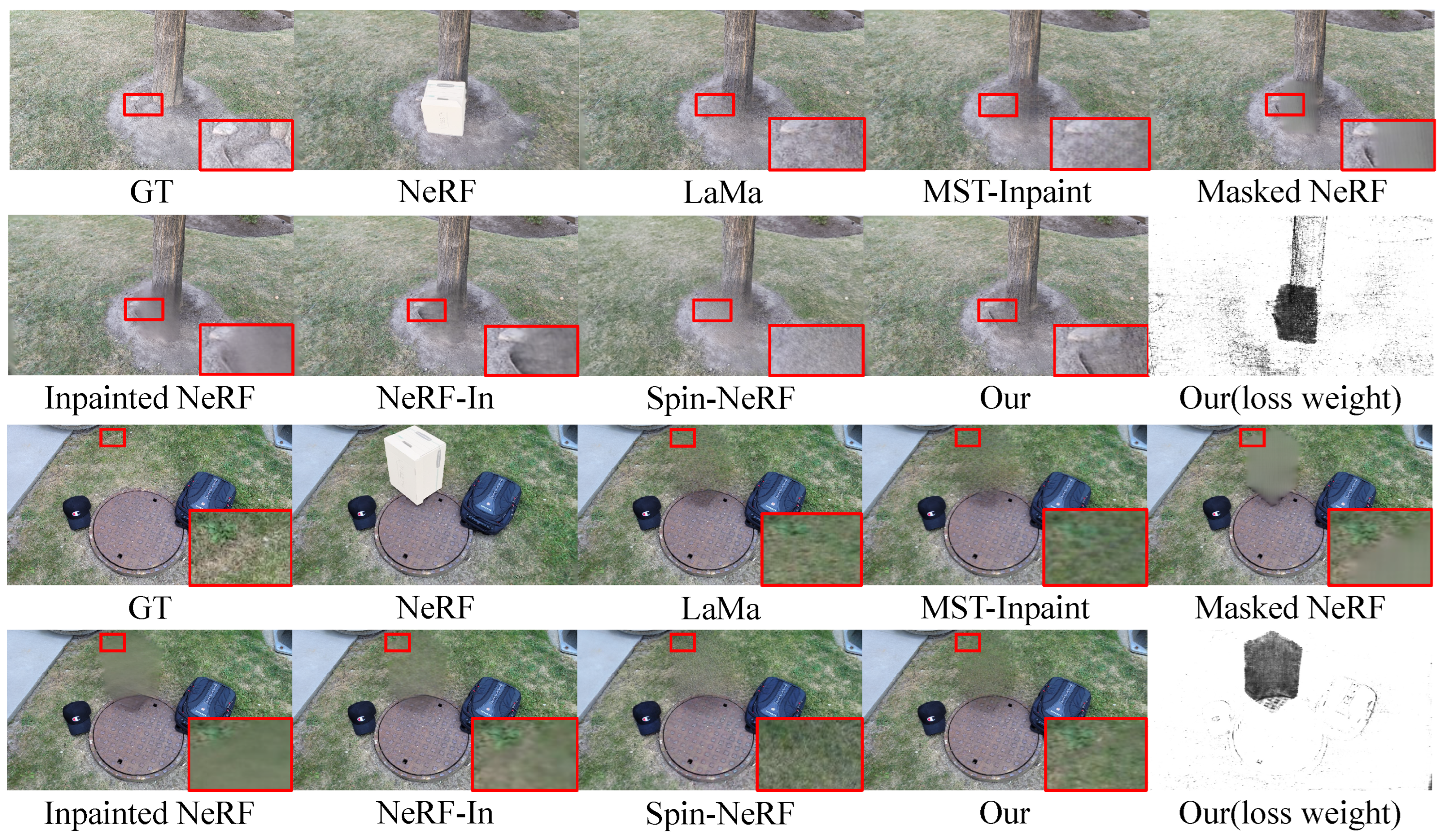
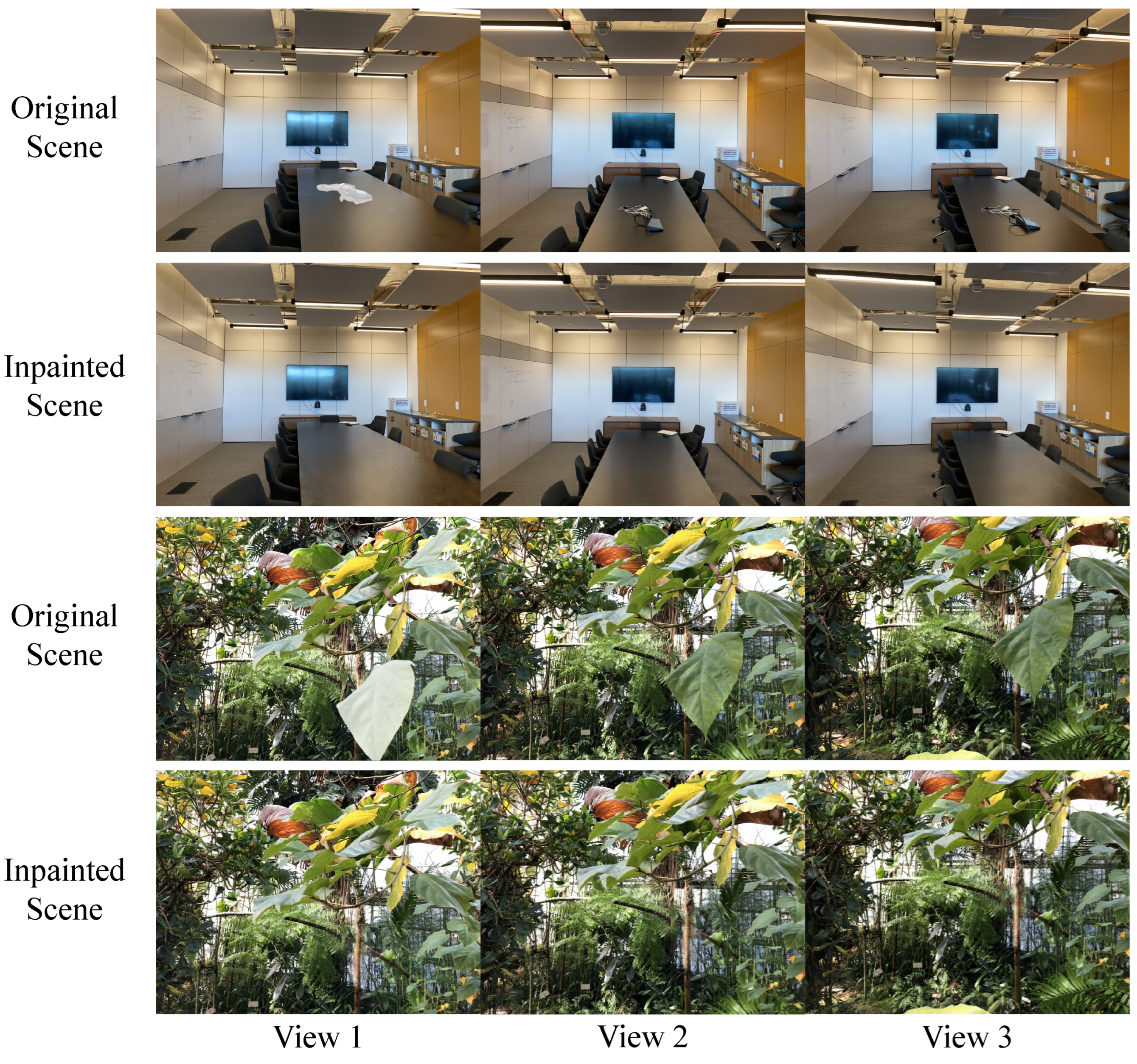
4.2.2. 3D-Consistent Scenes Inpainting

The Spin-NeRF and NeRF Object Removal datasets were used for the quantitative evaluation of the inpainting results of our proposed method against the baselines.

Table 2. Quantitative comparison of inpainted results with baselines. ↑ means higher value is better, while ↓ means lower value is better. Bold font indicates the best, and underlining indicates the second-best. Our method either secures the top spot or stands as the second-best across all metrics, presenting a distinct advantage over the baselines.

	Spin-NeRF Dataset				NeRF Object Removal Dataset
Mothed	LPIPS↓	FID↓	SSIM↑	GSMD↓	LPIPS↓	FID↓	SSIM↑	GSMD↓
LaMa [29]	0.0362	98.4	0.9452	0.0717	0.0483	90.3	0.9235	0.0837
MST-Inpaint [26]	0.0549	147.7	0.9440	0.0791	0.0775	118.6	0.9250	0.1012
Masked NeRF [1]	0.0612	210.2	0.9477	0.1084	0.0815	159.7	0.9341	0.1092
Inpainted NeRF [1]	0.0554	141.8	0.9475	0.0947	0.0743	167.0	0.9268	0.1118
NeRF-In [17]	0.0566	122.8	0.9481	0.0869	0.0727	103.5	0.9335	0.0933
Spin-NeRF [18]	0.0365	118.9	0.9451	0.0770	0.0543	114.4	0.9269	0.1012
Ours	0.0351	99.2	0.9480	0.0701	0.0480	81.7	0.9336	0.0788

highlights the superiority over all other NeRF-based inpainting models in LPIPS and FID. This signifies that our method can achieve good inpainting results, which is in line with human visual perception. SSIM was slightly lower than that of some baselines, although the gap was so small that it could be considered to be at the same level. Masked NeRF and Inpainted NeRF produced low scores in perceptual metrics. The former lacks inpaint supervision, resulting in hollow areas. The latter relies on the MSE loss, which prevents it from fitting data. Spin-NeRF closely trailed our method but exhibited a lower score on SSIM. This divergence might be attributed to its error in using the pure perception loss. It is worth noting that our method was closer to the 2D inpainting method LaMa in terms of perceptual metrics, which outputs our 2D inpainting priors. The model proposed in this paper can adeptly extract the features of 2D inpainting and extend its capabilities to 3D scenes. Considering all the metrics collectively, the proposed method emerges with distinct advantages over other baselines in the NeRF inpainting task.

A further qualitative analysis of the baselines was performed by presenting the visualization results. The focus of the comparison was primarily on 3D baselines, while the results of the 2D baselines LaMa and MST-Inpaint were used as references.

From the two scenes illustrated in Figure 5, our method preserved parts of the background occluded by target objects, such as the twigs in the tree scene and the weeds in the manhole cover scene. This result from our approach integrating all the view information when rendering the background, ensuring these regions are displayed without undergoing restoration treatments. NeRF-In achieved a somewhat similar effect by utilizing only inpainted regions of one view and the background of others. However, this approach lacks multi-view supervision in the inpainted regions, leading to blurred outputs. Spin-NeRF lost these details completely, while Masked NeRF preserved these details but produces hollow-looking images. Inpainted NeRF lost part of the true background. Remarkably, our method excelled by achieving both good preservation of real background details and good restoration results, while other baselines achieved one of them at most.

The functioning of dynamic loss weights is elucidated in Figure 6 through the visualization of the loss weights for the uncertainty branch. Darker regions represent higher weights against the adversarial loss and lead to more texture-level restoration, whereas lighter regions represent higher weights of the color loss, which is believed to be able to better restore the structure. Empirical observations showed that 2D inpainting models, including LaMa, tend to yield more consistent inpainting results for regions with clear and regular structures, as seen in the mesh and fence in Figure 6. Conversely, texture-rich regions are more inclined to perceptual-level inpainting, varying across different views. Our method recognized both inpainted results through the uncertainty branch, and further achieved a balance between structure and texture through dynamic weights. Hence, our method was able to obtain sharper edges and recover their texture information in appropriate regions. As regards the baseline methods, NeRF-In led to blurry results due to single-view supervision. Spin-NeRF suffered from ambiguous structural information because of the perceptual loss, and Inpainted NeRF performed worse in restoring vegetation texture.

The multi-view results of the proposed method are shown in Figure 7. In the first room scene, our model tackled the challenges posed by viewpoint-dependent effects, where smooth surfaces led to drastic color changes due to viewpoint movement. In fact, the uncertainty branch outputs of these regions were not high, signifying the proposed model’s ability to discern whether color changes stem from incorrect 2D inpainting or actual light reflections from the real scene. In the second scene, the region of the occlusion was large, and a lot of details would be lost by direct inpainting at the 2D level. Our model first employed a mask optimization step to retain more real information, such as part of the vegetation behind the leaves. This reduced the 3D inconsistency that may be brought about by the 2D inpainting phase. Finally, the results following the training with dynamic weights showcase enhanced inpainting, which is particularly noticeable in the improved inpainting of the tree trunk structure and the restoration of the surrounding vegetation texture.

4.3. Ablation Studies

Table 3. Quantitative comparison of the segmentation results with baselines. ↑ means higher value is better, while ↓ means lower value is better. Bold font indicates the best. Ablation results on the Spin-NeRF dataset. The metrics underscore the contribution of each component of our architecture towards improving the final results.

Method	LPIPS↓	FID↓	SSIM↑	GSMD↓
Our	0.0351	99.2	0.9480	0.0701
Our (w/o Mask Optimization)	0.0363	103.3	0.9469	0.0730
Our (w/o ${\mathcal{L}}_{adv}$)	0.0532	138.3	0.9478	0.0932
Our (w/o ${\mathcal{L}}_{MSE}$)	0.0426	110.6	0.9464	0.0756
Our (with Static Weights)	0.0382	114.7	0.9477	0.0752

shows the different components used in the ablation experiments and their comparative results. The complete architecture proposed in this paper obtained optimal results in all metrics. Omitting the first stage of mask optimization resulted in a large decrease in SSIM, indicating that mask optimization markedly aids the rendered image and mask pairs in retaining more background information. In addition, a comparison of the dynamic weights was performed. Three control groups were established: one without the adversarial loss, one without the MSE color loss, and one assigning equal static weights (0.5) to both losses. Using the loss without ${\mathcal{L}}_{adv}$ yielded blurred renderings, resulting in lower Lpips and FID scores. Conversely, exclusively employing the adversarial loss led to a substantial drop in SSIM and GSMD. While equal weighting of both losses generated better results, their metrics still trailed those achieved through dynamic weighting. We cannot deny that there may be a certain fixed weight that can work well in a particular scene, but dynamic weighting can obtain proper hyperparameters automatically for different scenes at the patch level.

Figure 8 shows the qualitative results of the ablation experiments. The impact of mask optimization was mainly compared in the first and second scenes. Notably, scenes processed with mask optimization effectively preserved details such as bushes and real flowers, while scenes lacking mask optimization showcased texture artifacts. This highlights the efficacy of the mask optimization module in retaining real information. The results of the training strategy based on dynamic weighting were compared in the third scene. It can be seen that the proposed complete method preserved good structures, such as table edges, while also generating appropriate textures. However, when the adversarial loss was removed, the texture details of the scene became blurry. Similarly, removing the MSE color loss severely weakened the structure, emphasizing the design intent of this paper where the color loss guides the structure and the adversarial loss guides the texture. Additionally, experiments employing static loss weights failed to produce satisfactory inpainted results in the third scene. The proposed method exhibited enhanced performance across different scene settings. The metrics and visualization of the ablation experiments affirm the pivotal role each part of the method in this paper plays in improving the experimental results.

4.4. Limitations

The proposed method also features some limitations. Since the method uses a 2D inpainting model as priors, the results for NeRF depend heavily on the same priors. The LaMa used in this paper occasionally disregards structural aspects and performs texture inpainting, resulting in, for example, a gradual texture artifact in the public seat in Figure 9. Thus, our model might also result in such errors. In addition, owing to the absence of lighting modeling, the method in this paper has flaws in handling shadows, and in some cases, remnants of shadows persist in the scene after object removal. Some recent works are very inspiring, such as the 3D Gaussian-based method that can perform relighting and have high expressive power [56]. Decoupling illumination has a positive effect on shadow removal. We hope to address these issues in future work.

5. Conclusions

In this paper, we propose a NeRF inpainting architecture that can effectively remove target objects from scenes and obtain reasonable results. The method in this paper orchestrates a two-stage process to realize inpainting. In the initial training stage, a mask branch and an uncertainty branch are integrated into the base NeRF for background rendering and mask optimization, fully exposing the background details of the training view. In the inpainting training stage, the uncertainty branch serves as a 3D consistency measurement for the inpainted view, from which dynamic weights are computed to balance the color loss and the adversarial loss. On this basis, the results are well inpainted at both the structure and texture levels. Quantitative and qualitative experiments were conducted to demonstrate the superiority of the proposed method over previous methods. It outperforms all 3D baselines in terms of perceptual metrics, and also has an advantage in structural metrics. In addition, it was experimentally demonstrated that the added components all notably enhance the overall model performance. Nevertheless, the work in this paper still has some limitations in terms of the dependency on the 2D model and the removal of shaded areas, which will be overcome via further exploration in subsequent work.

References

1. Mildenhall, B.; Srinivasan, P.P.; Tancik, M.; Barron, J.T.; Ramamoorthi, R.; Ng, R. Nerf: Representing scenes as neural radiance fields for view synthesis. Commun. ACM 2021, 65, 99–106. [Google Scholar] [CrossRef]
2. Levoy, M. Display of surfaces from volume data. IEEE Comput. Graph. Appl. 1988, 8, 29–37. [Google Scholar] [CrossRef]
3. Müller, T.; Evans, A.; Schied, C.; Keller, A. Instant neural graphics primitives with a multiresolution hash encoding. ACM Trans. Graph. (ToG) 2022, 41, 1–15. [Google Scholar] [CrossRef]
4. Fridovich-Keil, S.; Yu, A.; Tancik, M.; Chen, Q.; Recht, B.; Kanazawa, A. Plenoxels: Radiance fields without neural networks. In Proceedings of the IEEE/CVF Conference on Computer Vision and Pattern Recognition, New Orleans, LA, USA, 18–24 June 2022; pp. 5501–5510. [Google Scholar]
5. Chen, A.; Xu, Z.; Geiger, A.; Yu, J.; Su, H. Tensorf: Tensorial radiance fields. In Proceedings of the European Conference on Computer Vision, Tel Aviv, Israel, 23–27 October 2022; Springer: Berlin/Heidelberg, Germany; pp. 333–350. [Google Scholar]
6. Yang, J.; Pavone, M.; Wang, Y. FreeNeRF: Improving Few-shot Neural Rendering with Free Frequency Regularization. In Proceedings of the IEEE/CVF Conference on Computer Vision and Pattern Recognition, Vancouver, BC, Canada, 17–24 June 2023; pp. 8254–8263. [Google Scholar]
7. Jain, A.; Tancik, M.; Abbeel, P. Putting nerf on a diet: Semantically consistent few-shot view synthesis. In Proceedings of the IEEE/CVF International Conference on Computer Vision, Montreal, QC, Canada, 10–17 October 2021; pp. 5885–5894. [Google Scholar]
8. Kuang, Z.; Luan, F.; Bi, S.; Shu, Z.; Wetzstein, G.; Sunkavalli, K. Palettenerf: Palette-based appearance editing of neural radiance fields. In Proceedings of the IEEE/CVF Conference on Computer Vision and Pattern Recognition, Vancouver, BC, Canada, 17–24 June 2023; pp. 20691–20700. [Google Scholar]
9. Bao, C.; Zhang, Y.; Yang, B.; Fan, T.; Yang, Z.; Bao, H.; Zhang, G.; Cui, Z. Sine: Semantic-driven image-based nerf editing with prior-guided editing field. In Proceedings of the IEEE/CVF Conference on Computer Vision and Pattern Recognition, Vancouver, BC, Canada, 17–24 June 2023; pp. 20919–20929. [Google Scholar]
10. Fridovich-Keil, S.; Meanti, G.; Warburg, F.R.; Recht, B.; Kanazawa, A. K-planes: Explicit radiance fields in space, time, and appearance. In Proceedings of the IEEE/CVF Conference on Computer Vision and Pattern Recognition, Vancouver, BC, Canada, 17–24 June 2023; pp. 12479–12488. [Google Scholar]
11. Liu, Y.L.; Gao, C.; Meuleman, A.; Tseng, H.Y.; Saraf, A.; Kim, C.; Chuang, Y.Y.; Kopf, J.; Huang, J.B. Robust dynamic radiance fields. In Proceedings of the IEEE/CVF Conference on Computer Vision and Pattern Recognition, Vancouver, BC, Canada, 17–24 June 2023; pp. 13–23. [Google Scholar]
12. Haque, A.; Tancik, M.; Efros, A.A.; Holynski, A.; Kanazawa, A. Instruct-nerf2nerf: Editing 3d scenes with instructions. arXiv 2023, arXiv:2303.12789. [Google Scholar]
13. Zhang, K.; Kolkin, N.; Bi, S.; Luan, F.; Xu, Z.; Shechtman, E.; Snavely, N. Arf: Artistic radiance fields. In Proceedings of the European Conference on Computer Vision, Tel Aviv, Israel, 23–27 October 2022; Springer: Berlin/Heidelberg, Germany; pp. 717–733. [Google Scholar]
14. Gong, B.; Wang, Y.; Han, X.; Dou, Q. RecolorNeRF: Layer Decomposed Radiance Field for Efficient Color Editing of 3D Scenes. arXiv 2023, arXiv:2301.07958. [Google Scholar]
15. Yuan, Y.J.; Sun, Y.T.; Lai, Y.K.; Ma, Y.; Jia, R.; Gao, L. Nerf-editing: Geometry editing of neural radiance fields. In Proceedings of the IEEE/CVF Conference on Computer Vision and Pattern Recognition, New Orleans, LA, USA, 18–24 June 2022; pp. 18353–18364. [Google Scholar]
16. Goel, R.; Sirikonda, D.; Saini, S.; Narayanan, P. Interactive segmentation of radiance fields. In Proceedings of the IEEE/CVF Conference on Computer Vision and Pattern Recognition, Vancouver, BC, Canada, 17–24 June 2023; pp. 4201–4211. [Google Scholar]
17. Liu, H.K.; Shen, I.; Chen, B.Y. NeRF-In: Free-form NeRF inpainting with RGB-D priors. arXiv 2022, arXiv:2206.04901. [Google Scholar]
18. Mirzaei, A.; Aumentado-Armstrong, T.; Derpanis, K.G.; Kelly, J.; Brubaker, M.A.; Gilitschenski, I.; Levinshtein, A. SPIn-NeRF: Multiview segmentation and perceptual inpainting with neural radiance fields. In Proceedings of the IEEE/CVF Conference on Computer Vision and Pattern Recognition, Vancouver, BC, Canada, 17–24 June 2023; pp. 20669–20679. [Google Scholar]
19. Weder, S.; Garcia-Hernando, G.; Monszpart, A.; Pollefeys, M.; Brostow, G.J.; Firman, M.; Vicente, S. Removing objects from neural radiance fields. In Proceedings of the IEEE/CVF Conference on Computer Vision and Pattern Recognition, Vancouver, BC, Canada, 17–24 June 2023; pp. 16528–16538. [Google Scholar]
20. Ballester, C.; Bertalmio, M.; Caselles, V.; Sapiro, G.; Verdera, J. Filling-in by joint interpolation of vector fields and gray levels. IEEE Trans. Image Process. 2001, 10, 1200–1211. [Google Scholar] [CrossRef]
21. Li, K.; Wei, Y.; Yang, Z.; Wei, W. Image inpainting algorithm based on TV model and evolutionary algorithm. Soft Comput. 2016, 20, 885–893. [Google Scholar] [CrossRef]
22. Elad, M.; Starck, J.L.; Querre, P.; Donoho, D.L. Simultaneous cartoon and texture image inpainting using morphological component analysis (MCA). Appl. Comput. Harmon. Anal. 2005, 19, 340–358. [Google Scholar] [CrossRef]
23. Criminisi, A.; Pérez, P.; Toyama, K. Region filling and object removal by exemplar-based image inpainting. IEEE Trans. Image Process. 2004, 13, 1200–1212. [Google Scholar] [CrossRef] [PubMed]
24. Wang, W.; Niu, L.; Zhang, J.; Yang, X.; Zhang, L. Dual-path image inpainting with auxiliary gan inversion. In Proceedings of the IEEE/CVF Conference on Computer Vision and Pattern Recognition, New Orleans, LA, USA, 18–24 June 2022; pp. 11421–11430. [Google Scholar]
25. Liu, H.; Wan, Z.; Huang, W.; Song, Y.; Han, X.; Liao, J. Pd-gan: Probabilistic diverse gan for image inpainting. In Proceedings of the IEEE/CVF Conference on Computer Vision and Pattern Recognition, Nashville, TN, USA, 20–25 June 2021; pp. 9371–9381. [Google Scholar]
26. Cao, C.; Fu, Y. Learning a sketch tensor space for image inpainting of man-made scenes. In Proceedings of the IEEE/CVF International Conference on Computer Vision, Montreal, QC, Canada, 10–17 October 2021; pp. 14509–14518. [Google Scholar]
27. Dong, Q.; Cao, C.; Fu, Y. Incremental transformer structure enhanced image inpainting with masking positional encoding. In Proceedings of the IEEE/CVF Conference on Computer Vision and Pattern Recognition, New Orleans, LA, USA, 18–24 June 2022; pp. 11358–11368. [Google Scholar]
28. Yu, Y.; Zhan, F.; Lu, S.; Pan, J.; Ma, F.; Xie, X.; Miao, C. Wavefill: A wavelet-based generation network for image inpainting. In Proceedings of the IEEE/CVF International Conference on Computer Vision, Montreal, QC, Canada, 10–17 October 2021; pp. 14114–14123. [Google Scholar]
29. Suvorov, R.; Logacheva, E.; Mashikhin, A.; Remizova, A.; Ashukha, A.; Silvestrov, A.; Kong, N.; Goka, H.; Park, K.; Lempitsky, V. Resolution-robust large mask inpainting with fourier convolutions. In Proceedings of the IEEE/CVF Winter Conference on Applications of Computer Vision, Waikoloa, HI, USA, 3–8 January 2022; pp. 2149–2159. [Google Scholar]
30. Lugmayr, A.; Danelljan, M.; Romero, A.; Yu, F.; Timofte, R.; Van Gool, L. Repaint: Inpainting using denoising diffusion probabilistic models. In Proceedings of the IEEE/CVF Conference on Computer Vision and Pattern Recognition, New Orleans, LA, USA, 18–24 June 2022; pp. 11461–11471. [Google Scholar]
31. Yen-Chen, L.; Florence, P.; Barron, J.T.; Lin, T.Y.; Rodriguez, A.; Isola, P. Nerf-supervision: Learning dense object descriptors from neural radiance fields. In Proceedings of the 2022 International Conference on Robotics and Automation (ICRA), Philadelphia, PA, USA, 23–27 May 2022; pp. 6496–6503. [Google Scholar]
32. Viazovetskyi, Y.; Ivashkin, V.; Kashin, E. Stylegan2 distillation for feed-forward image manipulation. In Proceedings of the Computer Vision—ECCV 2020: 16th European Conference, Glasgow, UK, 23–28 August 2020; Proceedings, Part XXII 16. Springer: Berlin/Heidelberg, Germany, 2020; pp. 170–186. [Google Scholar]
33. Ho, J.; Jain, A.; Abbeel, P. Denoising diffusion probabilistic models. Adv. Neural Inf. Process. Syst. 2020, 33, 6840–6851. [Google Scholar]
34. Wang, P.; Liu, L.; Liu, Y.; Theobalt, C.; Komura, T.; Wang, W. Neus: Learning neural implicit surfaces by volume rendering for multi-view reconstruction. arXiv 2021, arXiv:2106.10689. [Google Scholar]
35. Oechsle, M.; Peng, S.; Geiger, A. Unisurf: Unifying neural implicit surfaces and radiance fields for multi-view reconstruction. In Proceedings of the IEEE/CVF International Conference on Computer Vision, Montreal, QC, Canada, 10–17 October 2021; pp. 5589–5599. [Google Scholar]
36. Zhi, S.; Laidlow, T.; Leutenegger, S.; Davison, A.J. In-place scene labelling and understanding with implicit scene representation. In Proceedings of the IEEE/CVF International Conference on Computer Vision, Montreal, QC, Canada, 10–17 October 2021; pp. 15838–15847. [Google Scholar]
37. Denker, J.; LeCun, Y. Transforming neural-net output levels to probability distributions. Adv. Neural Inf. Process. Syst. 1990, 3. Available online: https://proceedings.neurips.cc/paper_files/paper/1990/hash/7eacb532570ff6858afd2723755ff790-Abstract.html (accessed on 15 January 2024).
38. MacKay, D.J. A practical Bayesian framework for backpropagation networks. Neural Comput. 1992, 4, 448–472. [Google Scholar] [CrossRef]
39. Graves, A. Practical variational inference for neural networks. Adv. Neural Inf. Process. Syst. 2011, 24. Available online: https://proceedings.neurips.cc/paper_files/paper/2011/hash/7eb3c8be3d411e8ebfab08eba5f49632-Abstract.html (accessed on 15 January 2024).
40. Kendall, A.; Gal, Y. What uncertainties do we need in bayesian deep learning for computer vision? Adv. Neural Inf. Process. Syst. 2017, 30. Available online: https://proceedings.neurips.cc/paper_files/paper/2017/hash/2650d6089a6d640c5e85b2b88265dc2b-Abstract.html (accessed on 15 January 2024).
41. Martin-Brualla, R.; Radwan, N.; Sajjadi, M.S.; Barron, J.T.; Dosovitskiy, A.; Duckworth, D. Nerf in the wild: Neural radiance fields for unconstrained photo collections. In Proceedings of the IEEE/CVF Conference on Computer Vision and Pattern Recognition, Nashville, TN, USA, 20–25 June 2021; pp. 7210–7219. [Google Scholar]
42. Pan, X.; Lai, Z.; Song, S.; Huang, G. Activenerf: Learning where to see with uncertainty estimation. In Proceedings of the European Conference on Computer Vision, Tel Aviv, Israel, 23–27 October 2022; Springer: Berlin/Heidelberg, Germany, 2022; pp. 230–246. [Google Scholar]
43. Roessle, B.; Barron, J.T.; Mildenhall, B.; Srinivasan, P.P.; Nießner, M. Dense depth priors for neural radiance fields from sparse input views. In Proceedings of the IEEE/CVF Conference on Computer Vision and Pattern Recognition, New Orleans, LA, USA, 18–24 June 2022; pp. 12892–12901. [Google Scholar]
44. Cheng, H.K.; Tai, Y.W.; Tang, C.K. Rethinking space-time networks with improved memory coverage for efficient video object segmentation. Adv. Neural Inf. Process. Syst. 2021, 34, 11781–11794. [Google Scholar]
45. Lim, J.H.; Ye, J.C. Geometric gan. arXiv 2017, arXiv:1705.02894. [Google Scholar]
46. Mildenhall, B.; Srinivasan, P.P.; Ortiz-Cayon, R.; Kalantari, N.K.; Ramamoorthi, R.; Ng, R.; Kar, A. Local light field fusion: Practical view synthesis with prescriptive sampling guidelines. ACM Trans. Graph. (TOG) 2019, 38, 1–14. [Google Scholar] [CrossRef]
47. Zhang, R.; Isola, P.; Efros, A.A.; Shechtman, E.; Wang, O. The unreasonable effectiveness of deep features as a perceptual metric. In Proceedings of the IEEE Conference on Computer Vision and Pattern Recognition, Salt Lake City, UT, USA, 18–23 June 2018; pp. 586–595. [Google Scholar]
48. Heusel, M.; Ramsauer, H.; Unterthiner, T.; Nessler, B.; Hochreiter, S. Gans trained by a two time-scale update rule converge to a local nash equilibrium. Adv. Neural Inf. Process. Syst. 2017, 30. Available online: https://proceedings.neurips.cc/paper_files/paper/2017/hash/8a1d694707eb0fefe65871369074926d-Abstract.html (accessed on 15 January 2024).
49. Wang, Z.; Bovik, A.C.; Sheikh, H.R.; Simoncelli, E.P. Image quality assessment: From error visibility to structural similarity. IEEE Trans. Image Process. 2004, 13, 600–612. [Google Scholar] [CrossRef] [PubMed]
50. Xue, W.; Zhang, L.; Mou, X.; Bovik, A.C. Gradient magnitude similarity deviation: A highly efficient perceptual image quality index. IEEE Trans. Image Process. 2013, 23, 684–695. [Google Scholar] [CrossRef] [PubMed]
51. Krizhevsky, A.; Sutskever, I.; Hinton, G.E. Imagenet classification with deep convolutional neural networks. Adv. Neural Inf. Process. Syst. 2012, 25. Available online: https://proceedings.neurips.cc/paper/2012/hash/c399862d3b9d6b76c8436e924a68c45b-Abstract.html (accessed on 15 January 2024). [CrossRef]
52. Simonyan, K.; Zisserman, A. Very deep convolutional networks for large-scale image recognition. arXiv 2014, arXiv:1409.1556. [Google Scholar]
53. Rother, C.; Kolmogorov, V.; Blake, A. Interactive foreground extraction using iterated graph cuts, 2004. ACM Trans. Graph. 2004, 23, 309–314. [Google Scholar] [CrossRef]
54. Hao, Y.; Liu, Y.; Wu, Z.; Han, L.; Chen, Y.; Chen, G.; Chu, L.; Tang, S.; Yu, Z.; Chen, Z.; et al. Edgeflow: Achieving practical interactive segmentation with edge-guided flow. In Proceedings of the IEEE/CVF International Conference on Computer Vision, Montreal, BC, Canada, 11–17 October 2021; pp. 1551–1560. [Google Scholar]
55. Kobayashi, S.; Matsumoto, E.; Sitzmann, V. Decomposing nerf for editing via feature field distillation. Adv. Neural Inf. Process. Syst. 2022, 35, 23311–23330. [Google Scholar]
56. Liang, Z.; Zhang, Q.; Feng, Y.; Shan, Y.; Jia, K. GS-IR: 3D Gaussian Splatting for Inverse Rendering. arXiv 2023, arXiv:2311.16473. [Google Scholar]
Figure 1. Overall architecture of UC-NeRF consisting of two stages: The first stage, termed the initial training stage, involved training the initial radiance field, where the input image and mask were utilized, with the color loss L r g b and mask loss L m a s k with uncertainty to optimize color, depth, and mask images. The 2D model was then used for inpainting. In the second stage, namely, the inpainting training stage, uncertainty serves as a basis for evaluating 3D consistency. It was used to dynamically calculate the weights for the color loss L M S E and adversarial loss L a d v at the sampled pixels, and balance the inpainted results in terms of structure and texture.
Electronics 13 00448 g001
Figure 2. Model structure of the proposed UC-NeRF. The proposed UC-NeRF model extended the baseline model by incorporating two additional branches: the mask branch G m and the uncertainty branch G β . The radiance field achieved background rendering through G m , while optimized masks for areas to be inpainted were achieved using G β .
Electronics 13 00448 g002
Figure 3. Dynamic weights computed from the 3D consistency of the 2D inpainted views measured using the uncertainty branch. Two sampling examples are shown on the left. The red boxes represents two sampling patches. The blue boxes represents the uncertainty output value corresponding to the red boxes. The darker the color, the lower the uncertainty. The right side is the dynamic weight of the two sampling patches. The sampling patch with low uncertainty will get a higher MSE loss weight and a lower adversarial loss weight. Texture inpainting often results in high uncertainty value.
Electronics 13 00448 g003
Figure 4. Qualitative comparison of the segmentation against STCN and the results of mask optimization. The red boxes indicate the objects we wanted to segment. STCN was used as the segmentation priors for our model, and its output had errors. The results show that our model is robust against inaccurate priors, effectively correcting erroneous segmentation and obtaining accurate boundaries. Optimized views and masks are able to expose the occluded region and reduce the area requiring inpainting. In certain scenes, mask areas are nearly completely removed.
Electronics 13 00448 g004
Figure 5. Visualization comparison of manhole cover and tree scenes. The red boxes display the magnified details. NeRF displays the view without the objects being removed, and the white-covered areas indicate target objects. The boxed regions serve to illustrate that the proposed method can effectively address the 3D inconsistency issues evident in the restoration process while preserving more background details compared to other methods.
Electronics 13 00448 g005
Figure 6. Visualization comparison of mesh and fence scenes. The red boxes display the magnified details. The loss weight represents the visualization of dynamic weights in our method, where the darker color represents a higher weight for the adversarial loss and a lower weight for the color loss. The dynamic weights allow our method to more accurately identify areas requiring more structural or textural inpainting, resulting in final inpainting with clearer edges and perceptually plausible textures.
Electronics 13 00448 g006
Figure 7. Multi-view inpainted results. This figure primarily showcases two distinctive scenes: one with smooth surfaces exhibiting severe view-dependent effects, and the other with high complexity, leading to 3D inconsistencies in the 2D inpainted results. Our model achieved good performance across these scenarios.
Electronics 13 00448 g007
Figure 8. Quantitative comparison of the ablation experiments. The red boxes display the magnified details. The performance of the complete architecture is illustrated against four comparative experiment settings: without mask optimization, without adversarial loss, without MSE color loss, and with static weights. Mask optimization preserves the true background details, and dynamic weighting obtains a balance between texture and structure.
Electronics 13 00448 g008
Figure 9. Failure cases. The proposed method relies on the results of the 2D inpainting model. When the 2D model fails to inpaint properly, the proposed method may also generate similar failure results.
Electronics 13 00448 g009