Abstract
This paper examines the multi-scale super-resolution challenge of digital elevation models in remote sensing. A dual-domain multi-scale attention fusion network is proposed, which reconstructs digital elevation image details step-by-step using cascading sub-networks. This model incorporates components like the wavelet guidance and separation module, multi-scale attention fusion blocks, dilated convolutional inception module, and edge enhancement module to improve feature extraction and fusion capabilities. A new loss function is designed to enhance the model’s robustness and stability. Experiments indicate that the proposed model outperforms 15 benchmark models in PSNR, RMSE, MAE, , and metrics. In HMA data, The proposed model’s PSNR increases by 0.89 dB (~1.81%), and RMSE decreases by 1.22 m (~8.6%) compared to a state-of-the-art model. Compared to EDEM, which has the best elevation index, decreases by 0.79 (~16%). Additionally, the effectiveness and contribution of each DDMAFN component were verified through ablation experiments. Finally, on the SRTM dataset, The proposed model demonstrates superior performance even with interpolated degradation.
1. Introduction
With the rapid advancement of geographic information technology, digital elevation models (DEMs) representing topographic surface morphology are widely used in fields like geology, environmental studies, and urban planning. However, acquiring high-resolution DEM data is often hindered by high costs and long processing times due to equipment and technological limitations [1,2]. Additionally, DEM data often suffer from insufficient resolution, impacting their use in detailed terrain analysis. For example, the global-scale DEM product from SRTM [3] is a valuable resource for topographic studies, but its 30 m spatial resolution is insufficient for detailed geohazard terrain analysis. Therefore, improving DEM resolution using super-resolution techniques has become a key focus of current research.
In super-resolution processing of digital elevation models (DEMs), a key challenge is efficiently and accurately enhancing the detailed information of low-resolution DEM data to satisfy the growing demand for geospatial analysis. Conventional super-resolution methods, such as bicubic interpolation, can achieve satisfactory results in smooth-textured regions, but they are inadequate for terrain surfaces with complex textures and minor variations [4]. Such regions necessitate deeper neural networks to capture high-frequency features and details. However, single-depth networks often struggle to adapt to the variable texture properties in DEM data, leading to high computational costs and limited outcomes. Furthermore, real-world terrain surfaces display inherent roughness and localized variations, complicating the ability of neural networks to accurately fit high-frequency targets and intensifying the challenges of super-resolution reconstruction [5]. Consequently, developing a strategy that adaptively adjusts processing depth based on image content is essential for advancing DEM super-resolution technology.
This study focuses on the fine edge information and spatial continuity characteristics of digital elevation model (DEM) data. We utilize the multi-resolution analysis capabilities of the wavelet transform and design wavelet bootstrap and separation modules to capture high-frequency features and detailed information in the images. The Haar wavelet transform decomposes the feature map into sub-bands of different scales, each covering information within a specific frequency range. A network of varying depths is employed for each sub-band to extract features, enabling adaptive processing of complex and smooth texture regions. This approach provides richer feature information for subsequent parallel convolutional layer branching, enhancing the accuracy and detail of super-resolution processing. Additionally, progressive reconstruction sub-networks are designed to enable multi-scale feature extraction and fusion of DEM data. Within each sub-network, feature maps are finely optimized and fused through multiple steps, including convolution, wavelet transform, and residual joining. This enhances the network’s ability to detect small changes in the terrain surface and improves the accuracy of super-resolution reconstruction. To ensure that original features or output features from the previous sub-network are correctly fused at each key output node, we adopt cross-scale residual linking. This guarantees effective transmission and fusion of feature information, gradually approaching the high-resolution (HR) target. The contributions of this study can be summarized as follows:
- (1)
- Haar wavelet transform strategy for multi-view feature extraction: we introduce the Haar wavelet transform to separate high-frequency and low-frequency information in DEM data. This strategy aids the model in capturing complex texture and edge features in DEM data while enhancing the understanding of DEM data from multiple perspectives, significantly improving the accuracy and detail representation of super-resolution reconstruction;
- (2)
- Hybrid loss function for achieving low-frequency and high-frequency balance: To ensure the recovery of low-frequency details while reinforcing constraints on high-frequency edges, we designed a hybrid loss function. This function optimizes global and local features of the DEM image by comprehensively considering reconstruction errors of different frequency components, further improving the quality of the super-resolved DEM;
- (3)
- Comprehensive model performance evaluation and terrain adaptation analysis: To assess the generalization performance of DEM super-resolution models, we conducted a detailed comparative analysis of 15 models across diverse terrain environments, offering valuable reference for practical applications.
The remainder of the paper is organized as follows: Section 2 reviews technological advances related to DEM super-resolution. Section 3 presents the architecture and implementation details of the proposed model. Section 4 details the experimental data and training procedures. Section 5 discusses the experimental results, and Section 6 provides the conclusions.
2. Related Work
In the past decades, scholars have proposed various methods to improve DEM resolution [6,7], including traditional interpolation techniques like inverse distance weighting(IDW) [8], kriging [9,10], and bilinear interpolation [11]. The IDW [7] interpolation method assumes each sampling point has a local influence inversely proportional to the distance. Kriging [9,10] is a statistically based interpolation method estimating the value of an unknown pixel by considering spatial autocorrelation. Bilinear interpolation [11] uses the values of the four known surrounding pixels to calculate the value of the unknown pixel by linear interpolation. Since only local information is considered [4], these methods often fail to capture terrain changes and detailed features in larger areas, especially those with complex terrain changes. To better utilize global and non-local information, advanced super-resolution techniques need to be explored to capture terrain detail and complexity and address the challenges of complex terrain and large-scale data.
Recently, deep learning techniques, particularly Convolutional Neural Networks (CNNs) and Generative Adversarial Networks (GANs), have significantly advanced image processing, offering new solutions to the DEM super-resolution (SR) problem. CNN-based methods can automatically learn the mapping between low-resolution DEMs (LR) and high-resolution DEMs (HR) [12,13,14,15,16,17,18,19,20], while GANs generate high-quality SR data through adversarial learning [21,22,23,24,25,26,27,28,29]. Various CNN-based DEM super-resolution methods have emerged, showing strong potential in addressing complex urban terrain, multi-terrain feature fusion, and data-scarce areas [18,19,20]. Previous studies, such as RSPCN [30], EFDN [31], and EDEM [32], have improved the feature extraction abilities of super-resolution reconstruction networks by modifying the depth and stacking forms (cascading, cyclic, etc.) of the network structures. These studies improve the accuracy and efficiency of DEM reconstruction by designing various network structures [14,15,16,17,18,19,20]. CDEM [33] offers a continuous representation of terrain elevation data based on EDSR and can predict elevation values for arbitrary locations. However, global information, such as spatial autocorrelation, may be overlooked. In areas with significant negative spatial correlation, a single mapping function may be inadequate. Although CDEM employs L1 loss optimization, more advanced strategies may be necessary for specific terrain features and noise. The design of the loss function requires further exploration to enhance terrain feature learning and improve super-resolution reconstruction.
In recent years, many studies have focused on improving DEM resolution and preserving terrain features using GAN models. Specific GAN architectures, such as Deep Residual Generative Adversarial Network [23] and MASTER GAN [24], have significantly improved DEM reconstruction accuracy. Additionally, studies have explored applying existing image SR methods to DEM SR [21,22] and the potential of deep learning to improve DEM resolution globally. To improve model performance, researchers have increased the number of iterations, introduced perceptual loss [25,28], and proposed a two-step DEM SR method based on ESRGAN [27]. Studies have also demonstrated end-to-end deep learning approaches that generate DEMs from a single RGB image [26], reducing application limitations. A recent study introduced a new adversarial network [29] that combines polarized self-attention for discriminative spatial maps with densely connected multi-residue modules to generate HR DEMs. However, GANs may face issues like training instability and mode collapse when processing DEM data, leading to a lack of diversity and detailed features in the generated DEMs. Therefore, a new network architecture that fully utilizes multi-domain and multi-scale features is necessary to more effectively reconstruct elevation information of topographic landscapes.
With the ongoing advancement of multi-source data and feature extraction techniques, many new methods have emerged for DEM super-resolution and multi-source data fusion [34]. For example, the sparse representation with adaptive regularization can extract topographic information from sources like TanDEM-X [35] and combine it with other DEM data to generate high-resolution DEMs. DEM is characterized by large image sizes and substantial data volumes, leading to a significant conflict between the high speed of data acquisition and the low speed of processing and interpretation. Traditionally, the DEM processing mode required transmitting large amounts of data back to the ground for analysis, necessitating data compression and relying on high transmission bandwidth [36], which incurs significant costs. To recover terrain details, researchers designed a large-scale super-resolution Transformer network [37] that not only reconstructs coordinate information but also excels in learning DEM features. Additionally, a super-resolution architecture combining aerial images and a full convolutional neural network uses an attentional feedback mechanism [38] to intelligently fuse information from low-resolution DEMs and aerial images, generating highly realistic terrain. Besides the previously mentioned methods, many other deep learning approaches have emerged in DEM super-resolution [2,39,40,41,42,43,44]. These methods use innovative techniques to enhance the spatial resolution and detail accuracy of DEMs. To better utilize neighborhood information, Zhou [32] proposed a parallel filter with different receptive fields for feature extraction and fusion in super-resolution DEM reconstruction. Ma [14] introduced a feature enhancement network that combines global and local information, addressing checkerboard artifacts and loss of global information during network transmission. Additionally, transfer learning has been used to pre-train CNNs [40], which are then fine-tuned with DEM data to reconstruct high-resolution DEMs. Physical laws and geographic knowledge [42], nonlocal similarity algorithms [43], transformer-based methods [2,35], and single-image super-resolution techniques [44] have also been applied to DEM super-resolution.
3. Materials and Methods
In this section, we describe the DDMAFN architecture, focusing on its scalability and incremental upsampling. Next, we detail the sub-network design, including wavelet transform for feature separation and enhancement and parallel branches for spatial domain feature extraction. Additionally, we discuss the implementation details of the multi-scale attention fusion blocks (MAFBlock). Finally, we introduce a loss function designed to enhance the reconstruction quality of the proposed network.
3.1. Network Architecture
The DDMAFN structure is illustrated in Figure 1. The DDMAFN consists of a series of identical reconstruction sub-networks, each responsible for feature extraction and fusion at specific scales, aiming to incrementally achieve super-resolution reconstruction of low-resolution (LR) DEM data. To ensure the correct fusion of original features or output features from previous sub-networks at each key output node, a bicubic upsampling method is employed at the residual joints, except for the final reconstructed super-resolution (SR) DEM. The input LR DEM is converted into the original input feature map via convolution operation, which then enters the wavelet guidance module of the first reconstruction sub-network. In this module, the feature map is processed in both wavelet and spatial domains to capture more comprehensive image features. Next, the convolutionally processed feature map is fed into the MAFGroup with a cascade of 16 MAFBlock, fused with the convolutional feature map through residual links to enhance feature extraction and representation. Then, the feature map is further optimized and separated by the wavelet module. The optimized feature map is fused with the original input feature map to complete the first sub-network reconstruction. Entering the second reconstruction sub-network, the output of the first sub-network is fused with the original input feature map and upscaled for finer feature extraction. This sub-network repeats the feature extraction process of the first sub-network. The original input feature map and the output of the first sub-network are upscaled and fused with the output of the second sub-network to form a richer feature representation. Before entering the third sub-network, the original input feature map and the outputs of the first two sub-networks are upscaled, and feature fusion is performed to further integrate information at different scales. Finally, the output feature maps of the third sub-network are fused and convolved with the original input feature maps filtered by the Pixcelshuffle upsampling method four times to obtain super-resolution (SR) DEM results. This process enhances the resolution and detail of the DEM image through cross-scale feature fusion and gradual zoom-in strategy, obtaining SR results at multiple scales simultaneously.
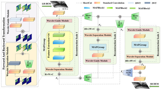
Figure 1.
Architecture of a dual-domain multi-scale attention fusion network. The three sub-networks are highlighted in pale green.
Following 3 × 3 convolution for feature extraction on the LR DEM, the information extraction process of 3 sub-networks can be described as follows:
where , and denote the output feature maps after passing through the 3 sub-networks, , , and correspond to the 3 sub-networks, which progressively process input data at different feature scales. represents an upsampling layer.
To address the issue of gradient vanishing, DDMAFN employs global residuals and local residuals to complete the reconstruction task by reusing features extracted from the preceding layer, as illustrated in the following equation:
where represents the sub-pixel convolutional upsampling layer.
3.2. Reconstruction Sub-Network
This sub-network, comprising six components, is employed to extract DEM image features.
3.2.1. Wavelet Guide Module
Accurately capturing and reconstructing detail and structural information in the image is crucial for DEM data super-resolution. Therefore, we designed a wavelet guide module that integrates spatial and wavelet domains to augment the model’s capacity to represent DEM data. Figure 1 illustrates the wavelet guide module. Initially, the input feature maps enter the wavelet guide module, where they undergo processing in the spatial and wavelet domains. Spatial domain processing involves feature extraction via a 3 × 3 convolutional layer. Meanwhile, processing in the wavelet domain captures image details and structure by decomposing the feature maps into high-frequency and low-frequency components using the Discrete haar wavelet transform (DWT). The high-frequency component contains image details, whereas the low-frequency component reflects the overall image structure. To reduce computational complexity and ensure consistent channel dimensions, wavelet coefficients undergo dimensionality reduction using 1 × 1 convolutional layers. Next, features from the spatial and wavelet domains are merged to produce the wavelet-guided output.
where and denote the input and output feature map of the current module, respectively. represents the concatenation function and represents the Haar wavelet positive transform function.
3.2.2. Wavelet Separation Module
Current DEM data super-resolution methods primarily rely on interpolation or single convolution operations for image reconstruction. Despite improved performance, these methods still struggle to capture the global structure and details of the image. Accurately recovering the complex structure and details of DEM data is crucial for enhancing DEM reconstruction quality. Therefore, the feature maps in the wavelet separation module (depicted in Figure 1) are divided into two parallel branches. One branch reconstructs wavelet domain features using the Inverse Wavelet Transform (IWT) to ensure accurate restoration, while the other branch reconstructs spatial domain features through 3 × 3 convolution and bicubic upsampling, maintaining dimensionality consistency with the wavelet domain output. The outputs of these two branches are fused to recover and enhance feature information from a spatial perspective, forming the final output.
where, represents the add function and represents the Haar Inverse Wavelet Transform function.
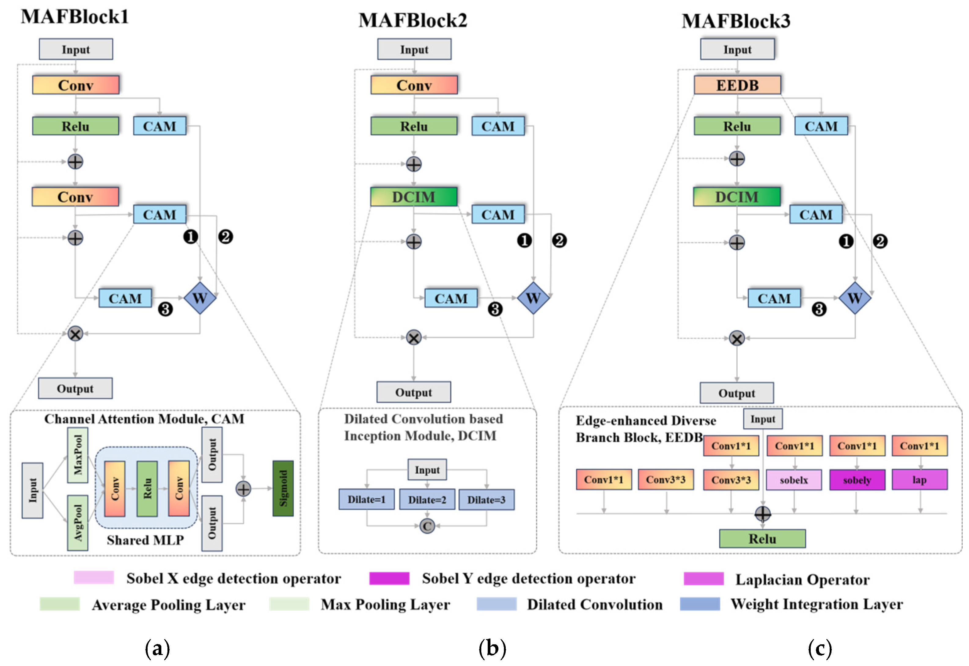
3.2.3. Multi-Scale Attention Fusion Blocks
MAF groups (MAFGroup), depicted in Figure 1, cascade three types of multi-scale attention fusion blocks (MAFBlock) with residual links to ensure deeper feature extraction, resulting in feature maps that integrate wavelet and spatial domains. During feature extraction, we introduce an additional residual link on top of the standard residual block, enabling more effective reuse of front-layer features. This design enhances the network’s ability to effectively utilize and transfer front-layer information, enriching background information for subsequent feature processing.
where 1/2/3 in represents three versions of MAFBlock (e.g., Figure 2), and ×16 represents a cascade of 16 MAFBlocks stacked atop one another. The MAFBlock comprises two core components: the feature extraction component and the multi-scale attention fusion.

Figure 2.
(a–c) are the three versions of the multi-scale attention fusion block.
The MAFBlock exists in three versions, all sharing a unified structural design to enhance feature extraction, adaptability, and robustness of the model.
The base block type combines convolutional operations with an attention mechanism. Initially, convolution processes the input feature map, dividing it into two branches. One branch enhances block representation with nonlinear features, facilitating richer feature transformation. The other emphasizes key features and suppresses redundant information via the Channel Attention Module (CAM) [45]. The CAM processing steps ensure proper weight assignment to the feature maps at different stages, enhancing the block’s ability to utilize and improve features of varying size and importance.
The second block type aims to broaden the perceptual range while preserving spatial information integrity. Introducing the dilated convolutional-based inception module (DCIM, as shown in Figure 2b) [46] captures features and details across different scales, enhancing multi-scale feature extraction. DCIM uses three 3 × 3 filters with dilation factors of 1, 2, and 3. Dilation is accomplished by inserting zeros between the filter elements to accommodate features of varying sizes and shapes in the image. Applying these dilation convolutions in parallel enables the modules to focus on features across different perceptual regions of the image, extracting multi-scale features in a single forward pass and capturing diverse image details and complexity.
Existing methods often overlook the importance of edge and detail information in DEM data processing. The third block type introduces an Edge Enhancement Diverse Branch Block in Figure 2c. This block enhances the multi-scale attention fusion module by prioritizing edge information extraction and emphasis, enriching the features. It contains six parallel branches, each performing specific operations on the input feature maps. The 1 × 1 convolution adjusts channel numbers and increases the non-linearity, while the 3 × 3 convolution captures a broader range of spatial information. These two are connected in tandem. Additionally, the module uses Sobel X and Y operators to extract horizontal and vertical edge features and employs the Laplace operator to extract second-order edge information, emphasizing detailed variations. The feature fusion from the six parallel branches provides a richer representation of edge-sensitive features for multi-scale attention fusion. This enables the network to leverage multiple convolutional operation scales and edge detection operators, enhancing edge feature sensitivity and representation and thereby improving super-resolution task performance.
3.3. Mutil-Scale Loss Function
Recognizing that the loss preserves image details more effectively than the loss and captures subtle variations in super-resolution tasks, this paper proposes a multiple supervised loss function based on the loss, with the goal of reconstructing pixel-level features and edge features at SR. To enhance the reconstruction of pixel-level information, this paper introduces a pixel-level loss function to facilitate multi-scale DEM reconstruction using the output characteristics of each sub-network.
where , , and are the HR sample data obtained by downsampling from the original high-resolution DEM data by factors of 1, 2, and 4, respectively. Additionally, the predicted SR results are reconstructed at three scales utilizing the feature outputs of each sub-network: , , , represents the pixel number of the DEM data.
To enhance edge information and ensure global model consistency, this paper introduces an edge loss, .
where , , and are extracted from the HR DEM using Sobel X, Sobel Y, and Laplace operators. , , and denote the results using Sobel X, Sobel Y, and Laplace operators in the SR DEM. The , , and denote the weighting parameters. represents the pixel number of the DEM data.
The final loss function combines pixel-level loss and edge-supervised loss , which are weighted and combined to guide the model in reconstructing a high-quality SR more comprehensively.
where and represent the weight coefficients of the pixel-level loss function and the edge-level loss function, respectively.
4. Experiments
4.1. Datasets
This study utilizes two datasets to construct data samples for the DEM SR model. The first dataset includes HR and LR samples from two different sources. HR data are sourced from the DAAC Asian Alpine Dataset (HMA), maintained by the U.S. National Snow and Ice Data Center (NSIDC), renowned for its reliability and detailed depiction of the Asian alpine. This dataset meticulously describes the intricate topographic features of the Tibetan Plateau and its surrounding region at an 8 m spatial resolution.
Conversely, LR data are sourced from the reliable ASTER GDEM, known for its broad coverage and consistent data quality, offering global elevation information at a 30 m resolution. ASTER GDEM covers the same latitude and longitude range as the HR data but at a reduced resolution. This combination aims to simulate real-world degradation processes and validate the model’s applicability. The second dataset exclusively employs Shuttle Radar Topography Mission (SRTM) data.
Bicubic downsampling of the SRTM HR data allowed us to acquire LR data at various scales. These data enable us to observe the model’s performance under diverse degradation scenarios.
4.2. Metrics
This paper evaluates the proposed method’s performance using Peak Signal-to-Noise Ratio (PSNR), Root Mean Square Error (RMSE), and Mean Absolute Error (MAE). Additionally, subjective judgments are made by integrating grayscale images with pseudo-3D images. It is important to note that we adjusted the PSNR calculation formula to suit the DEM’s characteristics, ensuring accurate assessment of pixel value differences between reconstructed and real data:
where is the maximum elevation value, is the minimum elevation value, and MSE, RMSE, and MAE are calculated by the formula:
where is the pixel value of the real HR DEM at the location and is the pixel value of the reconstructed SR DEM data at the same location . m and n represent the number of rows and columns of the image, respectively.
Additionally, given the crucial role of terrain feature consistency in DEM quality, this paper uses and as evaluation indexes to assess the model’s reconstruction performance on DEM data.
where represents the resolution of the DEM data, denotes the number of grids in the input data, and represents the elevation value of the i-th grid.
4.3. Data Preprocessing
During preprocessing, we curated two datasets. In the first dataset, we ensured accurate geospatial alignment and applied projection transformations to each HR and LR sample pair. We then selected 1055 LR-HR sample pairs from various regions, each containing rich topographic details. Subsequently, we partitioned 1039 samples for training and evaluation and 16 samples for testing purposes. To align with model training requirements, we uniformly cropped the HR data to a size of 512 × 512 pixels. Simultaneously, we resized the LR data after cropping to establish a 4× mapping ratio with the HR data. It is noteworthy that implementing the mapping relationship between HMA HR data and ASTER GDEM LR data under this simulation approach is highly challenging, akin to a more intricate degradation process. Conversely, for the second dataset, we chose 30 m SRTM data from flatland areas, measuring 7201 × 7201 pixels. To fit the model and enhance dataset diversity, we partitioned these data into 256 × 256-pixel patches and generated LR samples through downsampling with bicubic interpolation. Throughout this process, we rigorously screened the data quality and ultimately selected 659 high-quality DEMs, allocating 643 for training and 16 for testing. Additionally, we normalized the HR and LR datasets to establish a more stable and consistent database for model training.
4.4. Experimental Environment Settings
The experiments were conducted using Python 3.7, the Pytorch 1.11.0 framework, and NVIDIA GeForce RTX 3060 GPU. Adam optimizer was selected with an initial learning rate of 1 × 10⁻⁴, adaptively adjusted during training, and a batch size of 16. Additionally, we horizontally flipped or rotated the samples randomly to enhance sample diversity. In the super-resolution reconstruction experiments, DDMAFN was compared with Bicubic, SRCNN, VDSR, EDSR, SRGAN, DWSR, RCAN, SAN, SRFBN, EFDN, D-SRGAN, GISR, RSPCN, EDEM, and FEN models. Their performance was assessed based on PSNR, RMSE, MAE, , and metrics.
5. Results and Discussion
5.1. 4× Super-Resolution Results for GDEM to HMA Dataset
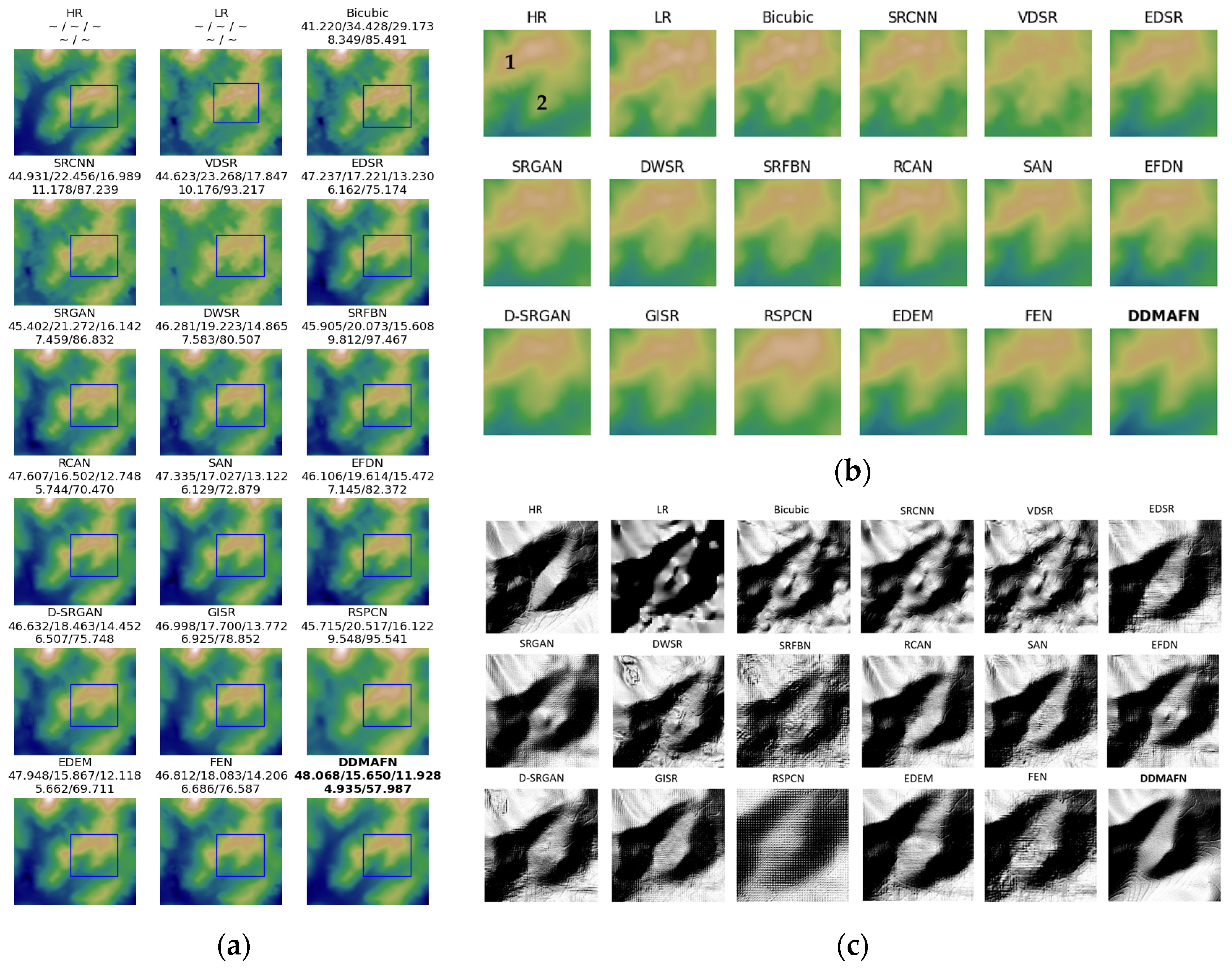
In the DEM SR task, HMA data served as the HR dataset, while GDEM data was used as the LR dataset. Table 1 shows that the bicubic interpolation method yields poor results in terms of PSNR, RMSE, and MAE. SRCNN, VDSR, and EDSR outperform bicubic interpolation across all metrics, demonstrating the effectiveness of deep learning in DEM SR tasks. Among the models involved tested, DDMAFN demonstrates the best performance. Additionally, DWSR, RCAN, SAN, SRFBN, EFDN, FEN, and EDEM also show outstanding performance. Their PSNR values range from 45.97 to 49.10, RMSE values from 14.25 to 20.51, and MAE values from 10.96 and 15.71. Although these models perform slightly lower than that of DDMAFN, they still significantly improve over the bicubic interpolation methods. Notably, GAN-based methods (e.g., SRGAN, D-SRGAN, and GISR) have relatively low PSNR. This may be because GAN methods focus more on the visual quality rather than faithfully reproducing original image details. Compared to the Bicubic method, DDMAFN improves in all three metrics. DDMAFN has a 21.35% higher PSNR than bicubic. Bicubic’s RMSE is 2.63 times higher, and its MAE is 2.98 times higher than DDMAFN’s. Table 1 illustrates that RCAN, EDEM, and DDMAFN perform excellently in slope and aspect errors. Specifically, DDMAFN achieves and values of 4.15° and 111.47° respectively.

Table 1.
4× SR results for the baseline model and DDMAFN on GDEM and HMA data.
Figure 3a displays the SR results for 16 different models. Figure 3b offers a magnified view of the specific area, whereas Figure 3c illustrates a zoomed hillshade map. A comparison between HMA data (HR) and GDEM (LR) reveals significant differences in mountaintop texture, particularly evident in the labeled region (1) in Figure 3b. Across the 16 model hillshade maps, it is evident that the Bicubic method fails to effectively reconstruct region (1), resulting in an outcome closer to the LR data. Similarly, the SRCNN and VDSR methods do not significantly enhance the result, exhibiting confusing textures in the region (2). Conversely, EDSR and EDEM outperform SRCNN and VDSR in the convolutional model, exhibiting fewer brown areas and a texture closer to resembling the HR image, thus demonstrating significant improvement. SRGAN, representing the GAN-based SR model, does not significantly outperform EDSR on the result map. The DWSR method employs a combination of frequency and wavelet domain features but exhibits blurred texture treatment in the region (2). The RCAN, SAN, EFDN, GISR, RSPCN, FEN, and DDMAFN methods deviate from the HR data in the shape of region (1), yet in region (2), the deviation is reduced, and they are closer to the HR data. Figure 3c reveals that the hillshade produced by Bicubic, SRCNN, and VDSR closely resembles the LR data but deviates significantly from the HR data. Conversely, methods like EDSR, SRGAN, DWSR, SRFBN, RCAN, SAN, EFDN, GISR, FEN, and EDEM are closer to the HR data in terms of hillshade appearance, albeit with some texture streaking issues. Specifically, DWSR and SRFBN exhibit more fragmented terrain depiction. Additionally, the RSPCN and FEN models exhibit a checkerboard effect, somewhat diminishing the quality of reconstruction. Conversely, DDMAFN results closely resemble HR data, allowing for better recovery of the local texture details and edge information while preserving the overall image structure consistency.
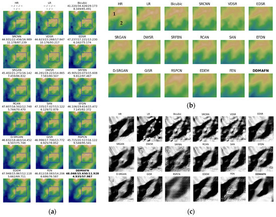
Figure 3.
4× SR results for the baseline model and DDMAFN on GDEM and HMA data. (a) is the SR results, (b) is the zoomed-in region(1 and 2 represent areas of significant variation), and (c) is the hillshade maps in the zoomed-in region.
5.2. 4× Super-Resolution Results on SRTM Dataset
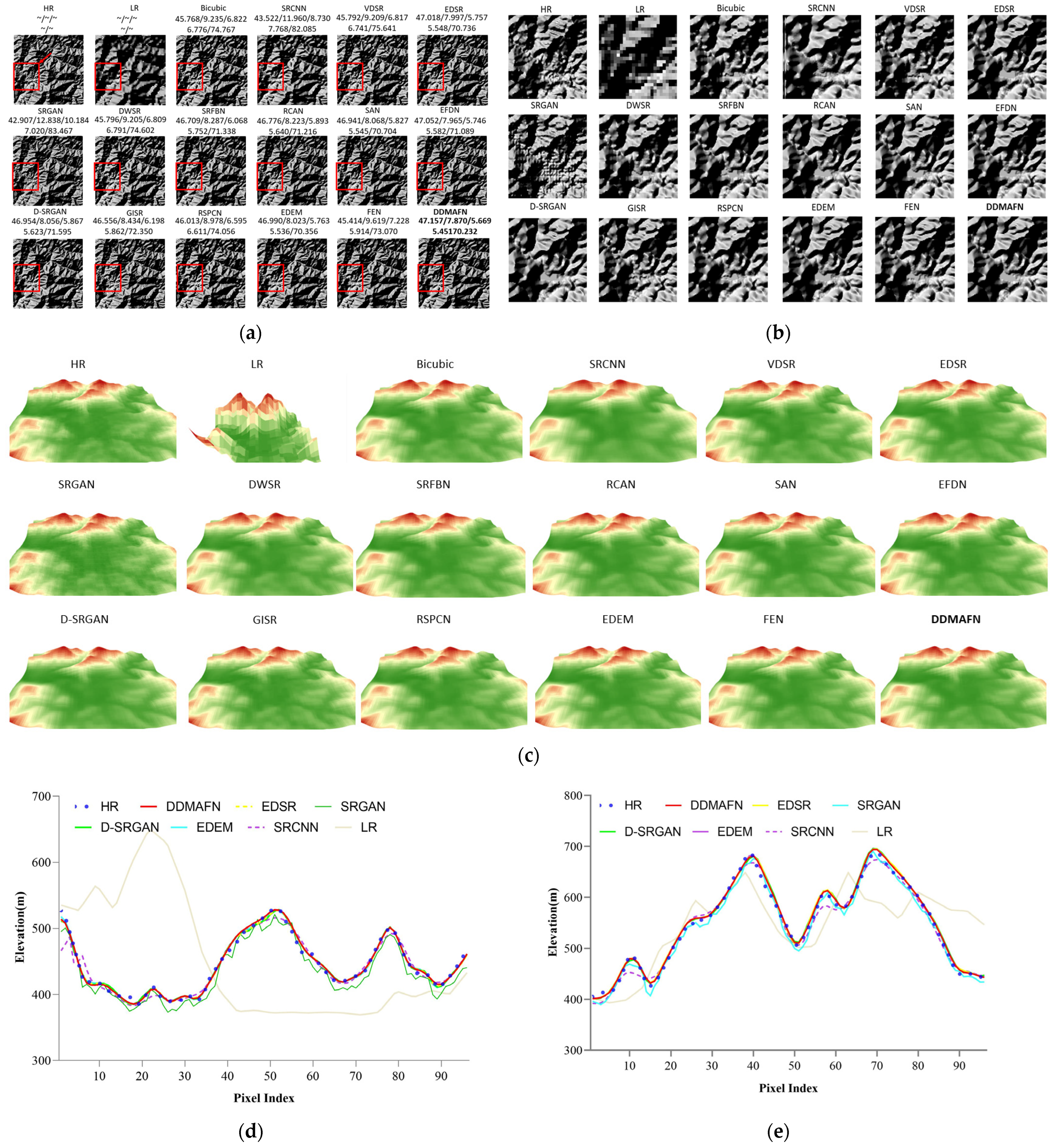
Table 2 presents the results of the 4× SR models on the SRTM data. Deep learning models generally outperform the Bicubic method, with VDSR and DWSR enhancing the deep network’s performance and marginally increasing the PSNR. RCAN, SAN, SRFBN, EFDN, EDEM, and DDMAFN all perform excellently, with PSNR values close to or above 48.50 and low RMSE and MAE. DDMAFN achieves the highest PSNR of 48.80 and the lowest RMSE of 6.70. Notably, EDSR, EDEM, and DDMAFN have similar PSNR, RMSE-elevation, and MAE-elevation values, maintaining the best results. However, DDMAFN, like EDSR and EDEM, has a low value, indicating good performance in restoring terrain slope. Additionally, DDMAFN achieves a low value, further verifying its advantages in maintaining the terrain’s spatial structure. SRGAN performs the poorest performance among the three metrics, with the lowest PNSR of 43.27 and the highest RMSE and MAE of 12.27 and 9.96, respectively. Additionally, the SRFBN has the best performance, with an MAE value of 4.68. By comparison, SRCNN, VDSR, DWSR, D-SRGAN, and GISR perform mediocrely in PSNR, RMSE, and MAE metrics. Additionally, and indexes show that these models still have room for improvement in feature extraction and reconstruction ability when processing DEM data. DDMAFN improves PSNR by 5.54 over SRGAN, while SRGAN’s RMSE is about 1.83 times that of DDMAFN, and its MAE is 2.13 times that of SRFBN.
Table 2.
4× SR results for the baseline model and DDMAFN on SRTM data.
Figure 4a displays the hillshade maps generated by 16 models for the DEM SR results, while Figure 4b provides a zoomed-in view of a partial area of the hillshade. Figure 4c presents a 3D visualization of the red-marked region, while Figure 4d and Figure 4e display graphs of the cross-section containing 11 rows and 13 columns, respectively. Generally, the 16 models can produce terrain features that closely resemble the HR data, indicating a high level of reconstruction capability. However, in some of the regional observations, we observed that the LR maps lacked topographic information, making it challenging to discern topographic details compared to the HR data. Comparing the hillshade maps of these 16 models, we observe that the Bicubic method better maintains the basic morphology consistent with the HR data, although significant differences exist in the details of the hillshade. The morphology differences between the SRCNN method and the HR data are considerable, with many fine-grained features left unrevealed. While the VDSR method excels in fine-grained features, it generates numerous pseudo-topographies compared with the HR hillshade maps, affecting the reconstruction accuracy. The EDSR method has similar issues, along with the EDSR, SRGAN, SRFBN, D-SRGAN, and GISR methods, which suffer from the mesh texture problem, further deteriorating the reconstruction quality. Furthermore, the false texture generated by the SAN method on the left side is a notable issue. The hillshade maps generated by EDSR, RCAN, EFDN, EDEM, and DDMAFN closely resemble the HR data and exhibit relatively better reconstruction quality. While they may not perfectly capture the features of the fine-grained terrain on the upper left side, these three methods effectively represent terrain features close to the HR data and demonstrate high reconstruction accuracy, especially in the high mountain part on the lower right side. Three-dimensional visualization (Figure 4c) further validates the DDMAFN model’s performance across diverse terrains, with reconstructed terrains closely resembling the actual high-resolution data in morphology and texture. A comparison of cross-section plots (Figure 4d,e) reveals that super-resolution models deviate at sharp elevation changes, while in flat regions with gradual changes, all models accurately fit the DEM HR curve. In contrast, the DDMAFN model fits the DEM HR curve more precisely, highlighting its superiority in detail preservation.
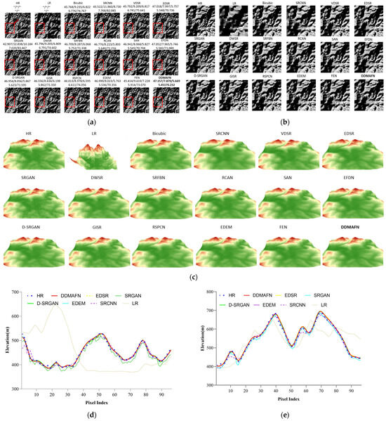
Figure 4.
4× SR results for the baseline model and DDMAFN on SRTM data. (a) is the hillshade map of SR results, and (b) is the hillshade map of the zoomed-in region (Corresponds to the red-boxed area in figure (a)).(c) is a 3D visualization of (b). (d) Represents the cross-section curve in row 11 of region (b). (e) Represents the cross-section curve in column 3 of region (b).
5.3. Ablation Experiments and Discussion
5.3.1. Effectiveness of Sub-Network Structure
To assess the proposed sub-network’s efficacy in multi-scale SR, we initially identified the experiment’s key scale factors: 2× and 8×. In the 2× model, we reduced the final sub-network to extract low magnification image features, whereas, in the 8× model, we appended an additional sub-network final one to capture high magnification image details.
- (1)
- Effectiveness of Sub-Networks with 2× Super-Resolution on SRTM Dataset
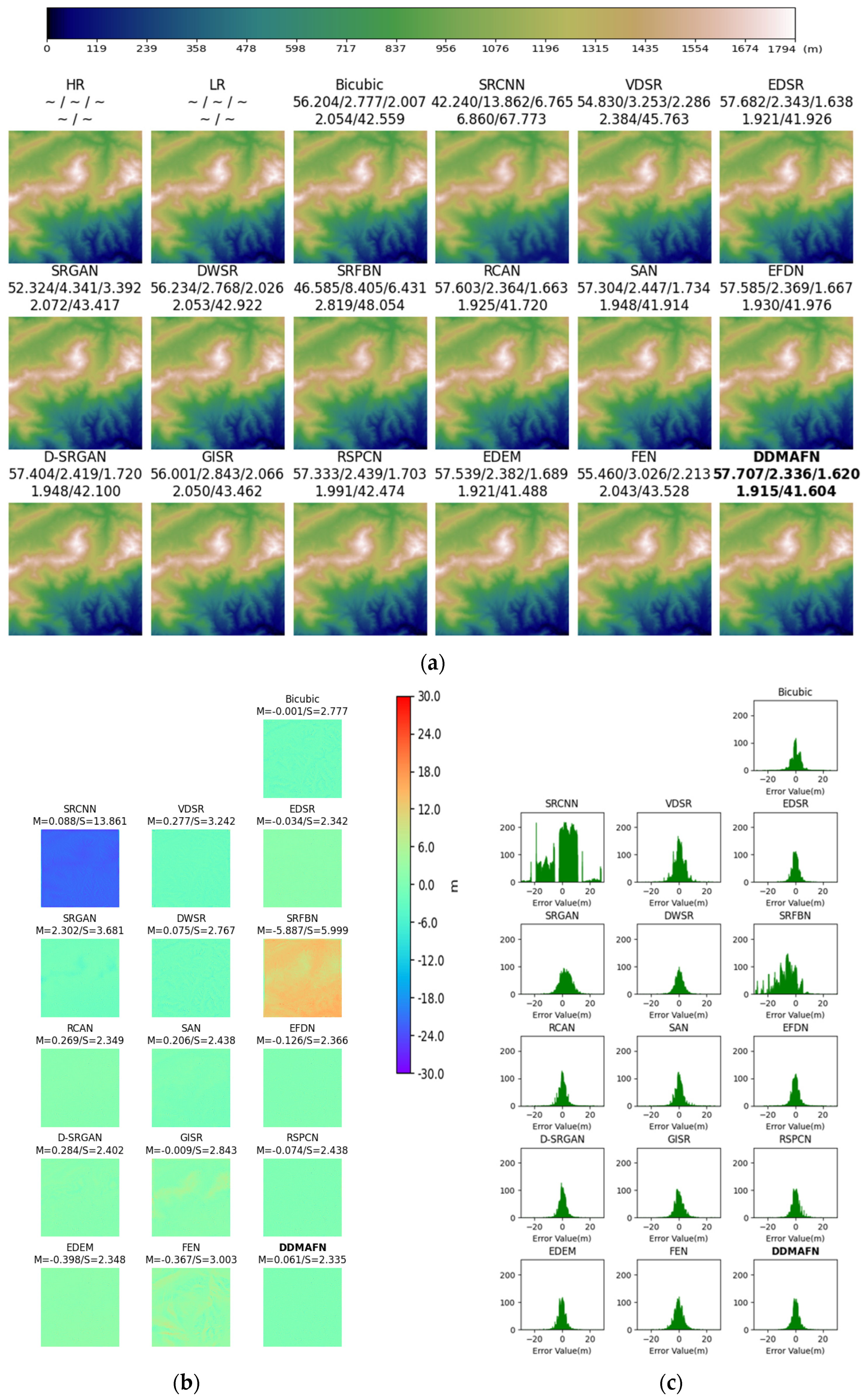
Table 3 displays the 2× SR results after removing the final sub-network (as depicted in Figure 1). In terms of PNSR, the EDSR, RCAN, EDEM, and DDMAFN models exhibit similar values, with RCAN slightly outperforming others at 57.13. Additionally, the Bicubic method demonstrates a relatively higher PNSR of 55.58, whereas the SRCNN yields the lowest PNSR of 45.44. Despite the simplicity and relatively high PSNR (55.58) of the traditional Bicubic algorithm, when compared with the 4× super-resolution reconstruction results of SRTM and HMA data, its limitations become evident. In terms of RMSE, the EDSR, RCAN, and DDMAFN models achieved the best performance, with identical values of 2.56, owing to their adoption of advanced network structures, showcasing the potential and advantages of deep learning in DEM data SR tasks. In terms of MAE, the EDSR, RCAN, and DDMAFN models demonstrate favorable performance, with DDMAFN achieving the lowest MAE value of 1.78. Upon comparing the performance of each model based on PNSR, RMSE, and MAE, the DDMAFN model closely approaches the best-performing model, achieving a PSNR of up to 57.11. Furthermore, it attains a low RMSE value of 2.56, demonstrating its robust capability to minimize reconstruction error. Particularly noteworthy is that DDMAFN attains the lowest MAE value of 1.78. Additionally, DDMAFN has exhibited good performance in the and metrics, suggesting its effectiveness and robustness in restoring terrain features in DEM data, owing to the advanced network structure design and multi-scale loss function constraints.
Table 3.
2× SR results for the baseline model and DDMAF on SRTM data.
From the 2× SR results depicted in Figure 5a, distinguishing differences between the 16 models visually is challenging. For further evaluation, error maps of the 2× SR images and the original HR images were calculated and plotted (Figure 5b) alongside a histogram of the error data (Figure 5c). Figure 5b,c collectively illustrates that the errors of DDMAFN, RSPCN, EDSR, and RCAN models are closer to zero, signifying their superior performance in the SR task and their ability to more accurately recover the HR image information. Nonetheless, the error distribution of SRCNN appears irregular, suggesting potential instability or inaccuracies in the reconstruction effectiveness of this model in certain regions. SRFBN errors predominantly exhibit negativity, whereas SRGAN errors lean towards positivity, indicating a potential bias or tendency in the reconstruction process of these models. RSPCN, FEN, and EDEM display mean error values close to 0 but negative, suggesting a limited extent of model generalization ability, resulting in slightly lower reconstruction results compared to the actual elevation value. The error distributions of SAN and D-SRGAN show similarities, possibly suggesting commonality in their SR strategies. While the distribution of positive and negative error values of GISR is normal, it lacks complete symmetry. Similarly to DWSR, its error distribution range is larger.
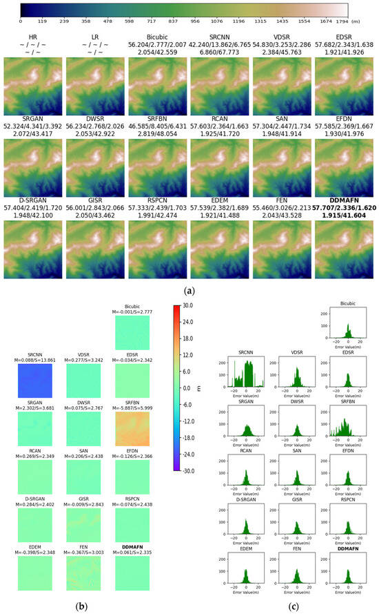
Figure 5.
2× SR results for the baseline model and DDMAFN on SRTM data. (a) is the SR results. (b) is error maps for HR-SR. (c) is the histogram of the error data.
- (2)
- Effectiveness of Sub-Networks with 8× Super-Resolution on SRTM Dataset
In the 8× SR experiments (Table 4), the Bicubic method yields a PSNR of 40.08, with RMSE and MAE values of 18.54 and 13.46, respectively. SRCNN exhibits a slightly lower PSNR than Bicubic at 39.45, accompanied by higher RMSE and MAE. VDSR and DWSR marginally enhance PSNR and reduce the errors. EDSR significantly improves PSNR to 41.15 while also substantially reducing RMSE and MAE. RCAN, SAN, SRFBN, EFDN, and DDMAFN achieved higher PSNR values and lower errors. Particularly, the DDMAFN achieves a PSNR of 41.24, with corresponding RMSE and MAE values of 16.11 and 11.49. It is notable that the SRGAN model performs inadequately in this task, exhibiting substantially lower PSNR value compared to other models and significantly higher RMSE and MAE. Additionally, considering DEM data’s emphasis on terrain slope and aspect, VDSR, SAN, EFDN, GISR, and DDMAFN models exhibit comparable performance in the and indexes, with DDMAFN demonstrating the best performance at 7.8 and 93.75, respectively. This further validates the strong terrain feature reconstruction ability of the sub-network, fully showcasing the robustness and effectiveness of the DDMAFN model in DEM data super-resolution reconstruction tasks. Overall, the DDMAFN model excels in image quality improvement, error control, and detail recovery in the 8× SR task.
Table 4.
8× SR results for the baseline model and DDMAFN on SRTM data.
Figure 6a displays the error maps of the SR results. Comparative analysis of the 8× SR images with the HR images revealed considerable variation in error distributions among the 16 models (Figure 6b). The error distributions of Bicubic, VDSR, RCAN, EDEM, D-SRGAN, EFDN, and DDMAFN are more centralized and closer to zero, possibly due to their superior preservation of original image information during reconstruction. Peaks of DWSR, EDSR, RSPCN, and DDMAFN are observed in the positive error region, while peaks of SRFBN, SAN, and EFDN emerge in the negative error region, possibly indicating variations in their reconstruction strategies or network structures, leading to some deviation. The larger and irregular error distribution of SRCNN may arise from its limitations in handling complex textures or details. The gradual increase in error from negative to positive for SRGAN may relate to its characteristics in balancing perceptual quality and pixel accuracy. Among all the models, GISR exhibits the smoothest error distribution, suggesting improved consistency and stability in processing different regions. Through 8× ablation experiments, we observe that the model structure proposed in this paper continues to yield satisfactory results in the SR task despite the addition of sub-networks, validating the model design’s effectiveness.
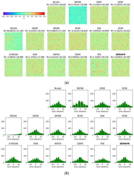
Figure 6.
The error maps of 8× SR results for the baseline model and DDMAFN on SRTM data. (a) is error maps for HR-SR. (b) is the histogram of the error data.
5.3.2. The Effect of Weights on Superscoring Results in Multi-Scale Attention Mechanisms
To explore the impact of various weight assignments in the multi-scale attention mechanism on the SR results, we conducted four sets of experiments for comparative analysis (displayed in Table 5). The weight assignments included (0:0:1), (0.1:0.1:0.8), (0.2:0.2:0.6), and a set of experiments that employed weight adaptive adjustment (Self-Adaption). In the experiment employing a weight adaptive adjustment allocation strategy, variance is utilized as an evaluation metric to dynamically assign more reasonable weights to each output. Experimental results indicate that in the (0:0:1) experiment, where the weights are entirely focused on the last scale, the model achieves a PSNR of 48.94, RMSE of 14.80, MAE of 11.35, with and values of 4.42 and 113.52, respectively. Adopting a balanced weight distribution method, like 0.2:0.2:0.6, significantly enhances the model’s performance, as reflected by the rise in PSNR value and the decline in RMSE and MAE, and . The model’s performance can be further optimized by moderately increasing the weight of the last branch, for instance, to 0.1:0.1:0.8. Although the RMSE value experiences a slight increase, it remains low, while the reduction in MAE suggests that the model optimizes other evaluation metrics while preserving high reconstruction quality. Notably, the weight allocation strategy in this group merits further reduction of the and indexes. This may be attributed to the last branch’s greater expressiveness in reconstructing specific details or terrain textures; thus, appropriately increasing its weight enhances the model’s performance. When the strategy of Self-Adaption was used, it did not bring the expected performance improvement.
Table 5.
4× SR results under different weight settings for DDMAFN.
5.3.3. Effectiveness of the Main Modules
Table 6 delineates the contributions and interactions among the DWT-IWT wavelet forward and inverse transforms, the MAFBlock, and the customized loss function in the SR task. Experimental results demonstrate that the DWT-IWT wavelet transform, as a fundamental component, significantly enhances SR performance and achieves satisfactory reconstruction quality when applied independently. In the absence of other key components, the MAFBlock exhibited poor performance, resulting in a decrease in PSNR to 42.20 and an increase in RMSE, MAE, , and to 30.98, 23.11, 46.31, and 155.58, respectively, suggesting that its benefits need to be complemented by other components for full realization. Additionally, the customized multi-scale loss function demonstrates its significance in enhancing SR performance. The combination of DWT-IWT and MAFBlock alone does not yield satisfactory performance improvement. However, the introduction of atop DWT-IWT notably enhances the model’s performance, with the PSNR increasing to 48.93 and RMSE and MAE, , and slightly decreasing. This indicates the effectiveness of integrating with the wavelet transform in super-resolution tasks. Introducing DWT-IWT, MAFBlock and simultaneously optimizes model performance, yielding the highest PSNR of 49.37 and the lowest RMSE and MAE of 14.02 and 10.80, respectively.
Table 6.
4× SR results for DDMAFN with different combinations of key modules.
5.3.4. Impact of Weight Settings on Network Performance
- (1)
- Effect of Edge and Pixel Loss Weight Setting on Super-Resolution Reconstruction Performance
In the super-resolution reconstruction of DEM data, topographic relief, and morphological changes are crucial for the fineness and accuracy of the reconstruction. Edge information, an important indicator of terrain changes, significantly impacts reconstruction quality. To focus the network model on edge information in DEM data, we set different weight ratios for edge loss and pixel loss in the loss function (as shown in Table 7). We compare the reconstruction results with real data in terms of edge features. Experimental results show significant performance improvement by increasing edge loss weight appropriately (e.g., = 0.9, = 0.1 in Experiment 12). While pixel loss also plays an important role, it mainly focuses on pixel-level differences and is less sensitive to reconstructing terrain details than edge loss. Decreasing pixel loss weight and increasing edge loss weight in the loss function helps the network model achieve better super-resolution reconstruction results. However, when the edge loss weight is too high (e.g., = 1, = 0 in Experiment 3), the network model’s performance decreases. Therefore, in super-resolution reconstruction of DEM data, adjusting the weight ratio of edge loss and pixel loss in the loss function is key to achieving high-performance reconstruction.
Table 7.
Results with different edge and pixel loss weight settings of .
- (2)
- Effect of Edge Detection Loss Weight Settings on Super-Resolution Reconstruction Performance
The weight settings (, , ) for different edge extraction methods (Sobel X, Sobel Y, and Laplace operator) in the edge loss function impact the super-resolution reconstruction of DEM data. As shown in Table 8, experiments show that model performance declines when edge weights in a specific direction are too high (e.g., Experiments 23 and 7). This may be because the model overemphasizes edge information in one direction, ignoring critical information in others, which affects the comprehensiveness and accuracy of the reconstruction results. Conversely, when the weight allocation is more balanced (e.g., Experiments 3 and 5), the model performs better, highlighting the importance of considering edge information from multiple directions. Additionally, the Laplace operator shows unique advantages in edge extraction. Experiments indicate better reconstruction results when Laplace operator weights are moderate (e.g., Experiments 5 and 19). This is because the Laplace operator captures second-order derivative information, which is sensitive to abrupt changes and details in the terrain data. Thus, reasonable utilization of edge information extracted by the Laplace operator enhances the fineness and clarity of super-resolution reconstruction in DEM data. Furthermore, the weight assignment of the Sobel operator in the x and y directions significantly impacts model performance. The Sobel operator extracts edge information horizontally and vertically, which is crucial for recovering topographic relief and orientation in DEM data. Experimental results show that balanced weights for Sobel X and Sobel Y better retain the topographic structure of the original DEM data (e.g., Experiments 3 and 11).
Table 8.
Results with different edge detection loss weight settings of .
5.3.5. Analysis of the Generalization Ability of Models across Different Terrains
In this paper, we propose the DDMAFN to address the challenge of super-resolution reconstruction of DEM data. First, we consider the complex topography of the Tibetan Plateau, which ranges from 3963.211 m to 7924.954 m in elevation, encompassing steep mountains, deep canyons, and varied geomorphic textures. The experimental results indicate that the DDMAFN achieves excellent reconstruction results even in this challenging environment. DDMAFN surpasses other deep learning models and the traditional Bicubic algorithm in several evaluation metrics, including peak PSNR, RMSE, MAE, and (see Table 1 for details). Meanwhile, DDMAFN demonstrates comparable performance to other state-of-the-art models, such as EDEM, EFDN, and SAN, on the SRTM dataset, which has a lower elevation (0–1794 m) and gentler terrain. Notably, although SRCNN slightly underperforms traditional interpolation algorithms due to its concise network structure, DDMAFN still maintains optimal performance in metrics such as RMSE, and . This demonstrates the strong generalization ability of the DDMAFN model in handling terrains of varying complexity.
Second, the visualization of the reconstruction results from GDEM to HMA data (Figure 3) shows that DDMAFN excels in restoring DEM terrain features and detailed textures, accurately reproducing the complex features in the original data. This high compatibility with high-resolution DEM data underscores its effectiveness. In the reconstruction of SRTM data (Figure 4), models like EDSR, RCAN, EFDN, EDEM, and DDMAFN generate mountain shadow maps similar to high-resolution DEM data, indicating a degree of generalization ability. Considering the results from both datasets, DDMAFN maintains stable performance in both complex and simple terrain conditions.
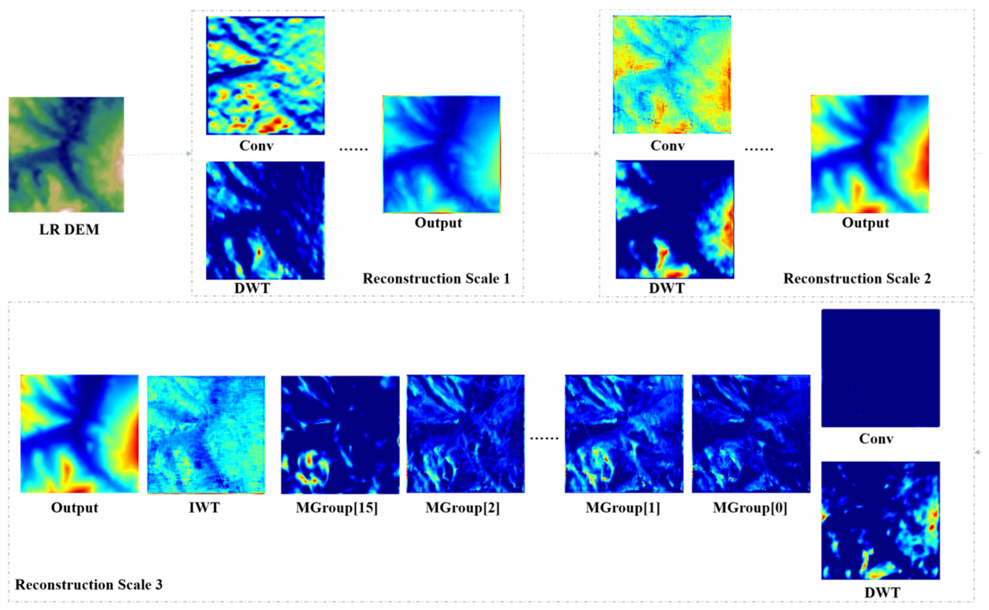
5.3.6. Interpretability Analysis
This section provides an in-depth exploration of the specific regions in the input LR DEM that are crucial for high-frequency detail extraction and edge enhancement. To achieve this, we utilize the Grad-CAM visualization technique to comprehensively visualize and analyze the core nodes in the DDMAFN. The results are presented in Figure 7.
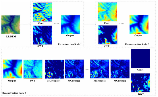
Figure 7.
Network Grad-CAM heat maps visualization.
By closely examining the heat maps of the Discrete Wavelet Transform (DWT) in the three reconstructed sub-networks, we observe that the region of interest in the wavelet guidance module demonstrates a refinement trend from coarse to fine as the network hierarchy progresses. In the first sub-network, the initial wavelet bootstrap module effectively guides the model in focusing on high-frequency detail features while providing a preliminary understanding of the overall structure of the LR DEM data. At this stage, the model demonstrates a fundamental ability to recognize the layout of each region within the LR DEM data. Simultaneously, the convolution operations in its parallel branches prioritize local feature extraction but lack the capacity to analyze global features. The combination of these two approaches creates a complementary effect, enabling the model to begin identifying key areas in the LR DEM data, such as contours of complex mountainous and flat regions, thereby enhancing its learning ability.
In the second reconstruction sub-network, the DWT component of the wavelet bootstrap module significantly enhances the model’s focus on high-frequency regions while also improving its ability to understand the overall structure. At this stage, edge delineation becomes clearer and more effective, allowing the model to better distinguish between different terrain features, such as peaks. Notably, although the LR DEM data may exhibit issues such as low quality and incoherent values due to acquisition conditions, the wavelet guidance module allows for finer focus on high-frequency details and edge features in the third sub-network, providing a deeper understanding of the numerical distribution of the LR DEM. This enhancement undoubtedly aids the model in performing high-frequency detail extraction and edge feature learning in subsequent modules. In complex terrains, this capability enables the model to more accurately reconstruct subtle features like undulations and slope changes, facilitating high-frequency detail extraction and edge feature learning in subsequent modules.
However, as the network depth increases, we observe a phenomenon: the convolutional branch of the wavelet guidance module increasingly neglects various regions of the DEM data, nearly losing its ability to recognize it in the final stage. To mitigate this unfavorable effect, we posit that the DWT in the wavelet bootstrap module is crucial, while the residual links serve a secondary auxiliary role.
Next, we analyze three different forms of the multi-scale attention module, MAFBlock, in the context of the third reconstruction sub-network. Although the different attention mechanism modules focus on the LR DEM data in slightly varied ways, they all demonstrate a strong emphasis on high-frequency regions and effectively delineate the regional layout of the LR DEM. Notably, in MAFBlock3, with the addition of the edge enhancement module, the model’s ability to control high-frequency details improves, enabling it to better perceive changes between high and low frequencies. Finally, by examining the overall output results of each sub-network, we find that as network depth increases, the model gains a more comprehensive understanding of the entirety while successfully capturing local high-frequency details and maintaining overall consistency, achieving an effective balance between the two.
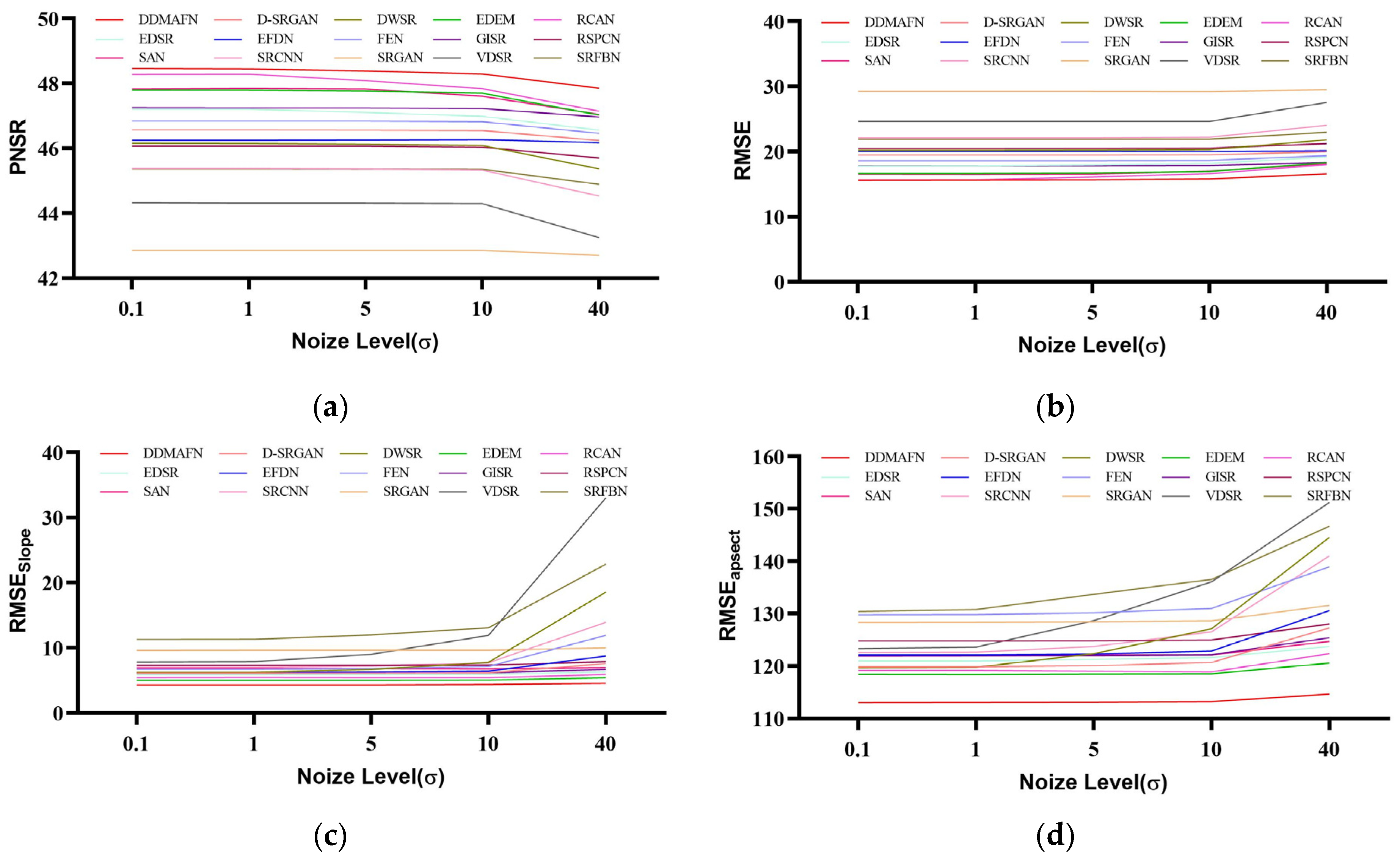
5.3.7. Sensitivity Analysis
In this section, we assess the performance of the DDMAFN model and comparison models under varying noise levels (Figure 8). Metrics including PSNR, RMSE, MAE, and were calculated by introducing Gaussian noise with variances ranging from 0.1 to 40 (shown in Figure 9). Experimental results indicate that while all models degrade with increasing noise, the DDMAFN model maintains optimal reconstruction accuracy. At low noise levels, model PSNR decreases slightly, and shows a limited increase, indicating strong robustness to low noise. At high noise levels, the DDMAFN model exhibits less PSNR reduction and smaller RMSE and MAE increases compared to the comparison models due to its multi-scale attention mechanism and progressive upsampling architecture, which effectively suppresses noise and minimizes information loss. Additionally, the SRGAN model shows the least change due to noise perturbation, possibly due to adversarial training, but demonstrates the weakest overall performance. Models like RCAN and EDEM experience greater performance degradation under high noise conditions but still outperform SRGAN.
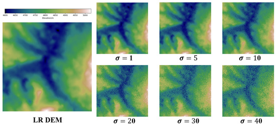
Figure 8.
Sample figure for different noise intensities.
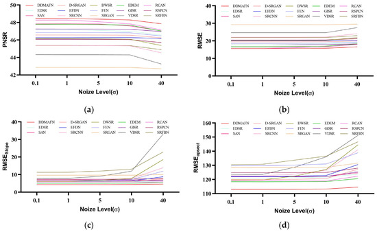
Figure 9.
Comparison of model performance under varying noise intensities. (a–d) are PNSR, RMSE, , and values for each model at different noise levels.
Figure 10 presents the terrain reconstruction results for hilly and flat regions, with the numerical values on each plot representing PSNR, RMSE, MAE, , and . In the hilly region, the DDMAFN model achieves a PSNR of 48.85 and an of 4.09, indicating its ability to capture terrain changes and learn these features during reconstruction. In the flat region, the DDMAFN model slightly improves, with PSNR increasing to 52.90 and decreasing to 3.21. This can be attributed to the flat region’s lower terrain variation, making it easier for the model to capture and replicate features. As shown in Figure 10, DDMAFN reconstructs terrain closest to the HR terrain, while the EDSR, SRGAN, SRFBN, D-SRGAN, and GISR methods exhibit varying levels of checkerboard effects across different terrains, reducing reconstruction quality. SRCNN and VDSR models show significant morphological differences and elevation errors compared to HR data. The SRCNN and VDSR models display considerable morphological differences from HR data, with significant elevation errors and failure to capture many fine-grained features. Hillshade maps generated by EDSR, RCAN, EFDN, EDEM, and DDMAFN across different terrains closely resemble those from HR DEM data, reflecting relatively high reconstruction quality. These differences may arise from varying model learning requirements for different terrain features.
Figure 10.
Terrain reconstruction results for mountain and flat regions. (a) terrain results for mountain areas, and (b) terrain results for flat areas.
5.3.8. Scalability Analysis
Table 9 summarizes the single inference time and model parameters for each model. As shown in the table, our proposed model achieves a competitive inference time of 0.75 s, comparable to other models such as EDSR, SRGAN, and FEN. Our model has 8.38 million parameters, placing it between models like VDSR (0.74 million parameters) and SRFBN (3.63 million parameters) in terms of complexity. Our model strikes a notable balance between inference speed and complexity, outperforming some models with fewer parameters (e.g., SRCNN, DWSR, RSPCN) while maintaining a reasonable inference time compared to more complex models (e.g., RCAN, SAN, EDEM). Achieving this balance is crucial for practical deployments, as it directly influences the model’s scalability and utility. Although models like RCAN and SAN are theoretically more accurate, their extensive parameters and long inference times may restrict their application in resource-constrained environments or those requiring rapid responses. In contrast, our model optimizes inference time and parameters, making it suitable for application scenarios that involve large volumes of DEM data requiring rapid computation.
Table 9.
Results of inference time and model parameters.
5.3.9. Application Analysis
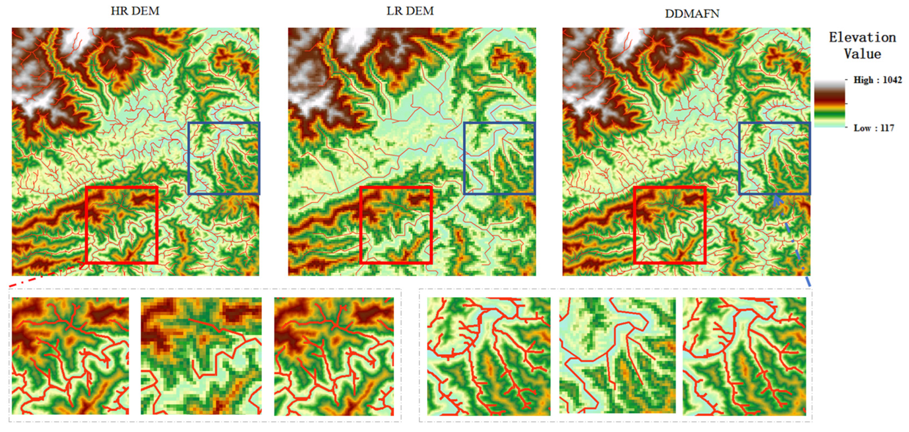
The river network is essential for depicting hydrological characteristics and plays a crucial role in water resources planning, utilization, optimal allocation, flood and drought control, tourism, and irrigation. Effective extraction of river network information is, therefore, critical. We employed the DDMAFN model to convert low-resolution DEM (LR DEM) data into high-resolution DEM (HR DEM) and subsequently extracted the river network from the resulting data. The results illustrated in Figure 11 represent the river networks extracted from the original HR DEM, LR DEM, and SR DEM, respectively. The extraction of the river network using low-resolution images often results in a significant loss of detailed information, as evidenced by the resulting images. However, the results obtained after super-resolution processing with the DDMAFN model demonstrate its effectiveness in recovering topographic information from low-resolution images. Notably, the river network structure extracted using the DDMAFN model exhibits a high degree of similarity to the results obtained from the original high-resolution DEM and maintains consistency in detail representation.

Figure 11.
Results of river network extraction. Detailed information regarding the red and blue areas is presented below, located on the left and right sides.
5.4. Limitations and Future Research
Currently, our model demonstrates strong performance, supported by sufficient paired data and high-quality samples. However, to enhance the model’s applicability and generalization capability, our future research will focus on improving DEM data quality, effectively incorporating physical information, and optimizing overall model performance.
The scarcity of the current paired DEM dataset significantly hampers the training scale and generalization capability of the model. To overcome this bottleneck, we will explore unsupervised training methods to maximize the utilization of limited data resources and enhance model performance. Meanwhile, we are developing an efficient void-filling model to address the data voids commonly encountered in HMA datasets from high mountain plateau regions. This model preprocesses DEM data to effectively fill data voids, thereby significantly enhancing its adaptability and robustness to abnormal environments.
For model optimization, we attempted to incorporate geographic information, such as slope and direction from the DEM data, as auxiliary inputs to enhance the DDMAFN model’s ability to reconstruct high-resolution terrain features. Experimental results indicated that this approach did not enhance model performance as anticipated; instead, it somewhat limited the model’s expressive capability. This finding highlights that merely combining geographically constrained information with DEM data does not guarantee improved performance. We further investigated incorporating slope and aspect information into the loss function to optimize the model using terrain feature constraints. However, experimental results demonstrate that these loss constraints tend to inhibit the effectiveness of other loss functions, such as perceptual and style losses. This suggests that while physical constraints can theoretically provide additional information, effectively integrating this information in practice remains an urgent challenge.
Given that DEM super-resolution reconstruction involves extensive data processing, improving efficiency while ensuring accuracy has become a key focus of our upcoming research. Striking a balance between model accuracy and computational cost presents a significant challenge. High-accuracy models yield superior results but often incur higher computational costs, such as longer inference times and increased model parameters. Conversely, models with lower computational costs, while more efficiently deployed, may compromise accuracy. Thus, finding the optimal balance between computational efficiency and model performance is crucial for practical applications. Accordingly, we will employ model compression techniques during the modeling process to reduce redundant parameters while ensuring accuracy, thereby achieving more efficient and accurate models to address the complex challenges encountered in practical applications.
6. Conclusions
This paper focuses on the DEM multi-scale super-resolution problem in remote sensing. We propose the DDMAFN model, which sequentially extracts features via a cascading sub-network and reconstructs DEM details using a progressive zoom-in strategy. Additionally, we introduce components, like the wavelet guidance module, multi-scale attention module, Channel Attention Module, dilation convolution perception module, and edge enhancement module, to enhance the network’s feature extraction and fusion capability. Experiments show that DDMAFN outperforms 15 state-of-the-art models in the DEM SR task, particularly excelling in PSNR, RMSE, MAE, and metrics. Furthermore, ablation experiments validated the effectiveness of the model components. In the SR task, experiments using HMA as high-resolution data and GDEM as low-resolution data show the deep learning model outperforms traditional methods. In both 2× and 8× SR experiments, DDMAFN performs well, effectively controlling the reconstruction error. In future work, we will explore more effective SR techniques to further improve DEM super-resolution reconstruction performance and quality.
Author Contributions
Conceptualization, B.H.; methodology, B.H. and X.M.; validation, B.H. and B.K.; formal analysis, B.W. and X.W.; data curation, X.M.; writing–initial draft, B.H. and X.M.; writing–reviewing and editing, B.K. and X.W. All authors have read and agreed to the published version of the manuscript.
Funding
This research was funded by the Natural Science Foundation of Sichuan Province (No. 2023NSFSC0243), the Talent Introduction Program of Chengdu University of Information Technology (No. KYTZ202261), the Shenzhen High-level Talent Research Startup Project (No. RC2024-003).
Data Availability Statement
The data presented in this study are available on request from the corresponding author.
Conflicts of Interest
The authors declare no conflicts of interest.
References
- Rossi, C.; Gernhardt, S. Urban DEM generation, analysis and enhancements using TanDEM-X. ISPRS J. Photogramm. Remote Sens. 2013, 85, 120–131. [Google Scholar] [CrossRef]
- Zhang, Y.; Zhang, Y.; Mo, D.; Zhang, Y.; Li, X. Direct Digital Surface Model Generation by Semi-Global Vertical Line Locus Matching. Remote Sens. 2017, 9, 214. [Google Scholar] [CrossRef]
- Scott Watson, C.; Kargel, J.S.; Tiruwa, B. UAV-Derived Himalayan Topography: Hazard Assessments and Comparison with Global DEM Products. Drones 2019, 3, 18. [Google Scholar] [CrossRef]
- Chen, G.; Chen, Y.; Wilson, J.P.; Zhou, A.; Chen, Y.; Su, H. An Enhanced Residual Feature Fusion Network Integrated with a Terrain Weight Module for Digital Elevation Model Super-Resolution. Remote Sens. 2023, 15, 1038. [Google Scholar] [CrossRef]
- Wu, H.; Ni, N.; Zhang, L. Lightweight Stepless Super-Resolution of Remote Sensing Images via Saliency-Aware Dynamic Routing Strategy. IEEE Trans. Geosci. Remote Sens. 2023, 61, 3236624. [Google Scholar] [CrossRef]
- Achilleos, G. The Inverse Distance Weighted interpolation method and error propagation mechanism—Creating a DEM from an analogue topographical map. J. Spat. Sci. 2011, 56, 283–304. [Google Scholar] [CrossRef]
- Rees, W.G. The accuracy of Digital Elevation Models interpolated to higher resolutions. Int. J. Remote Sens. 2000, 21, 7–20. [Google Scholar] [CrossRef]
- Shepard, D. A Two-Dimensional Interpolation Function for Irregularly-Spaced Data. In Proceedings of the 1968 23rd ACM National Conference, Las Vegas, NV, USA, 27–29 August 1968; pp. 517–524. [Google Scholar] [CrossRef]
- Cressie, N. The origins of kriging. Math. Geol. 1990, 22, 239–252. [Google Scholar] [CrossRef]
- Wackernagel, H. Ordinary kriging. In Multivariate Geostatistics: An Introduction with Applications; Springer: Heidelberg/Berlin, Germany, 2003; pp. 79–88. [Google Scholar] [CrossRef]
- Shi, W.Z.; Tian, Y. A hybrid interpolation method for the refinement of a regular grid digital elevation model. Int. J. Geogr. Inf. Sci. 2006, 20, 53–67. [Google Scholar] [CrossRef]
- Chen, Z.; Wang, X.; Xu, Z.; Hou, W. Convolutional neural network based dem super resolution. Int. Arch. Photogramm. Remote Sens. Spat. Inf. Sci. 2016, 41, 247–250. [Google Scholar] [CrossRef]
- Demiray, B.Z.; Sit, M.; Demir, I. DEM super-resolution with efficientNetV2. arXiv 2021, arXiv:2109.09661. [Google Scholar]
- Ma, X.; Li, H.; Chen, Z. Feature-Enhanced Deep Learning Network for Digital Elevation Model Super-Resolution. IEEE J. Sel. Top. Appl. Earth Obs. Remote Sens. 2023, 16, 5670–5685. [Google Scholar] [CrossRef]
- Jiao, D.; Wang, D.; Lv, H.; Peng, Y. Super-resolution reconstruction of a digital elevation model based on a deep residual network. Open Geosci. 2020, 12, 1369–1382. [Google Scholar] [CrossRef]
- Jiang, Y.; Xiong, L.; Huang, X.; Li, S.; Shen, W. Super-resolution for terrain modeling using deep learning in high mountain Asia. Int. J. Appl. Earth Obs. Geoinf. 2023, 118, 103296. [Google Scholar] [CrossRef]
- Jiang, L.; Hu, Y.; Xia, X.; Liang, Q.; Soltoggio, A.; Kabir, S.R. A Multi-Scale Mapping Approach Based on a Deep Learning CNN Model for Reconstructing High-Resolution Urban DEMs. Water 2020, 12, 1369. [Google Scholar] [CrossRef]
- Yue, L.; Shen, H.; Yuan, Q.; Zhang, L. Fusion of multi-scale DEMs using a regularized super-resolution method. Int. J. Geogr. Inf. Sci. 2015, 29, 2095–2120. [Google Scholar] [CrossRef]
- Zhang, Y.; Yu, W. Comparison of DEM Super-Resolution Methods Based on Interpolation and Neural Networks. Sensors 2022, 22, 745. [Google Scholar] [CrossRef]
- Zhou, A.; Chen, Y.; Wilson, J.P.; Chen, G.; Min, W.; Xu, R. A multi-terrain feature-based deep convolutional neural network for constructing super-resolution DEMs. Int. J. Appl. Earth Obs. Geoinf. 2023, 120, 103338. [Google Scholar] [CrossRef]
- Chantaveerod, A.; Woradit, K.; Seagar, A.; Limpiti, T. A Novel Catchment Estimation for Super-Resolution DEM With Physically Based Algorithms: Surface Water Path Delineation and Specific Catchment Area Calculation. IEEE Access 2023, 11, 70132–70152. [Google Scholar] [CrossRef]
- Dahal, A.; Van den Bout, B.; van Westen, C.J.; Nolde, M. Deep Learning-Based Super-Resolution of Digital Elevation Models in Data Poor Regions. 2022. Available online: https://eartharxiv.org/repository/view/4639/ (accessed on 30 August 2024).
- Deng, X.; Hua, W.; Liu, X.; Chen, S.; Zhang, W.; Duan, J. D-SRCAGAN: DEM Super-resolution Generative Adversarial Network. IEEE Geosci. Remote Sens. Lett. 2022; Early Access. [Google Scholar] [CrossRef]
- Mohammed, A.; Kashif, M.; Zama, H.; Ansari, M.A.; Ali, S. Master GAN: Multiple Attention is all you Need: A Multiple Attention Guided Super Resolution Network for Dems. In Proceedings of the IGARSS 2023—2023 IEEE International Geoscience and Remote Sensing Symposium, Pasadena, CA, USA, 16–21 July 2023; pp. 5154–5157. [Google Scholar] [CrossRef]
- Moreira, L.A.; Poelking, L.M.; Araki, H. Enhancing SRTM digital elevation models with deep-learning-based super-resolution image generation. Bol. Cienc. Geodesicas 2022, 28, e2022023. [Google Scholar] [CrossRef]
- Panagiotou, E.; Chochlakis, G.; Grammatikopoulos, L.; Charou, E. Generating Elevation Surface from a Single RGB Remotely Sensed Image Using Deep Learning. Remote Sens. 2020, 12, 2002. [Google Scholar] [CrossRef]
- Wu, Z.; Ma, P. ESRGAN-based DEM super-resolution for enhanced slope deformation monitoring in lantau island of Hong Kong. Int. Arch. Photogramm. Remote Sens. Spat. Inf. Sci. 2020, 43, 351–356. [Google Scholar] [CrossRef]
- Wu, Z.; Zhao, Z.; Ma, P.; Huang, B. Real-World DEM Super-Resolution Based on Generative Adversarial Networks for Improving InSAR Topographic Phase Simulation. IEEE J. Sel. Top. Appl. Earth Obs. Remote Sens. 2021, 14, 8373–8385. [Google Scholar] [CrossRef]
- Guo, T.; Mousavi, H.S.; Vu, T.H.; Monga, V. Deep Wavelet Prediction for Image Super-Resolution. In Proceedings of the 2017 IEEE Conference on Computer Vision and Pattern Recognition Workshops, Honolulu, HI, USA, 21–26 July 2017; pp. 104–113. [Google Scholar]
- Zhang, R.; Bian, S.; Li, H. RSPCN: Super-Resolution of Digital Elevation Model Based on Recursive Sub-Pixel Convolutional Neural Networks. ISPRS Int. J. Geo-Inf. 2021, 10, 501. [Google Scholar] [CrossRef]
- Wang, Y. Edge-enhanced Feature Distillation Network for Efficient Super-Resolution. In Proceedings of the 2022 IEEE/CVF Conference on Computer Vision and Pattern Recognition Workshops (CVPRW), New Orleans, LA, USA, 19–20 June 2022; pp. 777–785. [Google Scholar]
- Zhou, A.; Chen, Y.; Wilson, J.P.; Su, H.; Xiong, Z.; Cheng, Q. An Enhanced Double-Filter Deep Residual Neural Network for Generating Super Resolution DEMs. Remote Sens. 2021, 13, 3089. [Google Scholar] [CrossRef]
- Yao, S.; Cheng, Y.; Yang, F.; Mozerov, M.G. A continuous digital elevation representation model for DEM super-resolution. ISPRS J. Photogramm. Remote Sens. 2024, 208, 1–13. [Google Scholar] [CrossRef]
- Paul, S.; Gupta, A. SIRAN: Sinkhorn Distance Regularized Adversarial Network for DEM Super-resolution using Discrimi-native Spatial Self-attention. arXiv 2023, arXiv:2311.16490. [Google Scholar]
- Guan, L.; Hu, J.; Pan, H.; Wu, W.; Sun, Q.; Chen, S.; Fan, H. Fusion of public DEMs based on sparse representation and adaptive regularization variation model. ISPRS J. Photogramm. Remote Sens. 2020, 169, 125–134. [Google Scholar] [CrossRef]
- Rakhmanov, A.; Wiseman, Y. Compression of GNSS Data with the Aim of Speeding up Communication to Autonomous Vehicles. Remote Sens. 2023, 15, 2165. [Google Scholar] [CrossRef]
- Li, Z.; Zhu, X.; Yao, S.; Yue, Y.; García-Fernández, F.; Lim, E.G.; Levers, A. A large scale Digital Elevation Model super-resolution Transformer. Int. J. Appl. Earth Obs. Geoinf. 2023, 124, 103496. [Google Scholar] [CrossRef]
- Kubade, A.; Patel, D.; Sharma, A.; Rajan, K.S. AFN: Attentional feedback network based 3D terrain super-resolution. In Proceedings of the Asian Conference on Computer Vision, Kyoto, Japan, 30 November–4 December 2020. [Google Scholar] [CrossRef]
- Liu, C.; Du, W.; Tian, X. Lunar DEM Super-resolution reconstruction via sparse representation. In Proceedings of the 2017 10th International Congress on Image and Signal Processing, BioMedical Engineering and Informatics, Shanghai, China, 14–16 October 2017; pp. 1–5. [Google Scholar]
- Xu, Z.; Chen, Z.; Yi, W.; Gui, Q.; Hou, W.; Ding, M. Deep gradient prior network for DEM super-resolution: Transfer learning from image to DEM. ISPRS J. Photogramm. Remote Sens. 2019, 150, 80–90. [Google Scholar] [CrossRef]
- Zhang, X.; Zhang, W.; Guo, S.; Zhang, P.; Fang, H.; Mu, H.; Du, P. UnTDIP: Unsupervised neural network for DEM super-resolution integrating terrain knowledge and deep prior. Int. J. Appl. Earth Obs. Geoinf. 2023, 122, 103430. [Google Scholar] [CrossRef]
- Han, X.; Ma, X.; Li, H.; Chen, Z. A Global-Information-Constrained Deep Learning Network for Digital Elevation Model Super-Resolution. Remote Sens. 2023, 15, 305. [Google Scholar] [CrossRef]
- Xu, Z.; Wang, X.; Chen, Z.; Xiong, D.; Ding, M.; Hou, W. Nonlocal similarity based DEM super resolution. ISPRS J. Photogramm. Remote Sens. 2015, 110, 48–54. [Google Scholar] [CrossRef]
- Zhang, Y.; Zheng, Z.; Luo, Y.; Zhang, Y.; Wu, J.; Peng, Z. A CNN-Based Subpixel Level DSM Generation Approach via Single Image Super-Resolution. Photogramm. Eng. Remote Sens. 2019, 85, 765–775. [Google Scholar] [CrossRef]
- Woo, S.; Park, J.; Lee, J.-Y.; Kweon, I.S. CBAM: Convolutional block attention module. In Proceedings of the European Conference on Computer Vision (ECCV), Munich, Germany, 8–14 September 2018; pp. 3–19. [Google Scholar] [CrossRef]
- Shi, W.; Jiang, F.; Zhao, D. Single image super-resolution with dilated convolution based multi-scale information learning inception module. In Proceedings of the 2017 IEEE International Conference on Image Processing (ICIP), Beijing, China, 17–20 September 2017; IEEE: Piscataway Township, NJ, USA; pp. 977–981. [Google Scholar] [CrossRef]


Disclaimer/Publisher’s Note: The statements, opinions and data contained in all publications are solely those of the individual author(s) and contributor(s) and not of MDPI and/or the editor(s). MDPI and/or the editor(s) disclaim responsibility for any injury to people or property resulting from any ideas, methods, instructions or products referred to in the content. |
© 2024 by the authors. Licensee MDPI, Basel, Switzerland. This article is an open access article distributed under the terms and conditions of the Creative Commons Attribution (CC BY) license (https://creativecommons.org/licenses/by/4.0/).