L-GraphSAGE: A Graph Neural Network-Based Approach for IoV Application Encrypted Traffic Identification

Abstract

Recently, with a crucial role in developing smart transportation systems, the Internet of Vehicles (IoV), with all kinds of in-vehicle devices, has undergone significant advancement for autonomous driving, in-vehicle infotainment, etc. With the development of these IoV devices, the complexity and volume of in-vehicle data flows within information communication have increased dramatically. To adapt these changes to secure and smart transportation, encrypted communication realization, real-time decision-making, traffic management enhancement, and overall transportation efficiency improvement are essential. However, the security of a traffic system under encrypted communication is still inadequate, as attackers can identify in-vehicle devices through fingerprinting attacks, causing potential privacy breaches. Nevertheless, existing IoV traffic application models for encrypted traffic identification are weak and often exhibit poor generalization in some dynamic scenarios, where route switching and TCP congestion occur frequently. In this paper, we propose LineGraph-GraphSAGE (L-GraphSAGE), a graph neural network (GNN) model designed to improve the generalization ability of the IoV application of traffic identification in these dynamic scenarios. L-GraphSAGE utilizes node features, including text attributes, node context information, and node degree, to learn hyperparameters that can be transferred to unknown nodes. Our model demonstrates promising results in both UNSW Sydney public datasets and real-world environments. In public IoV datasets, we achieve an accuracy of 94.23%(↑0.23%). Furthermore, our model achieves an F1 change rate of 0.20%(↑96.92%) in $\alpha$ train, $\beta$ infer, and 0.60%(↑75.00%) in $\beta$ train, $\alpha$ infer when evaluated on a dataset consisting of five classes of data collected from real-world environments. These results highlight the effectiveness of our proposed approach in enhancing IoV application identification in dynamic network scenarios.

1. Introduction

With the pervasive reach of the Internet, ensuring robust network security has become paramount, particularly within the realm of smart transportation systems, where the Internet of Vehicles (IoV) plays a central role [1,2]. As IoV devices become increasingly integrated into traffic applications, they enhance connectivity and efficiency and expose critical infrastructure to heightened risks. This vulnerability is especially pronounced in the context of IoV. Data flow integrity and system operations are crucial for maintaining safe and efficient transportation networks. To effectively manage, monitor, and safeguard these IoV systems, it is essential to accurately identify network flows and applications, thereby ensuring the security and reliability of smart transportation infrastructures [3,4].

As traditional Deep Packet Inspection (DPI) introduces high overheads and fails when the traffic is encrypted [5], machine learning (ML)-based flow identification is emerging as a promising security paradigm. Accordingly, many ML-based mechanisms have been proposed. For instance, Fu et al. [6] proposed Whisper, a real-time malicious flow identification system based on ML, which utilizes frequency domain features to achieve high accuracy and high throughput. Although Whisper utilizes sequence information represented by the frequency domain and achieves bounded information loss, its representation is incomplete due to the lack of flow interactivity. Zhu et al. [7] proposed Robust critical fine-tuning (RiFT), a novel approach to enhance generalization without compromising adversarial robustness. Li et al. [8] introduced FOAP, a systematic solution that achieves fine-grained user action identification within an open-world environment. However, the scenario of FOAP is confined to a single network, primarily focusing on close-range wireless environments.

Deep learning (DL) is also an effective classification method for encrypted network flow. Giampaolo et al. [9] provided the first attempt to employ Few Shot Learning (FSL) to classify mobile application encrypted flows. Although the two-way flow features of the convection are processed in [9], the interaction features between the flows are not fully considered. Moreover, many existing works, such as [10,11,12,13,14,15,16], have utilized deep learning techniques for traffic identification, providing valuable insights for practical applications. Recently, Lo et al. [17] proposed E-GraphSAGE, an IoV identification system based on graph neural networks (GNNs). E-GraphSAGE aims to identify network intrusions in the IoV by utilizing the structural features of graph data to capture edge features and topological information.

Overall, the works mentioned above are the basis and key to network management and surveillance, as their objective is to organize various flows into different classes for IoV device identification. Consequently, these works have yielded favorable outcomes within their specific contexts.

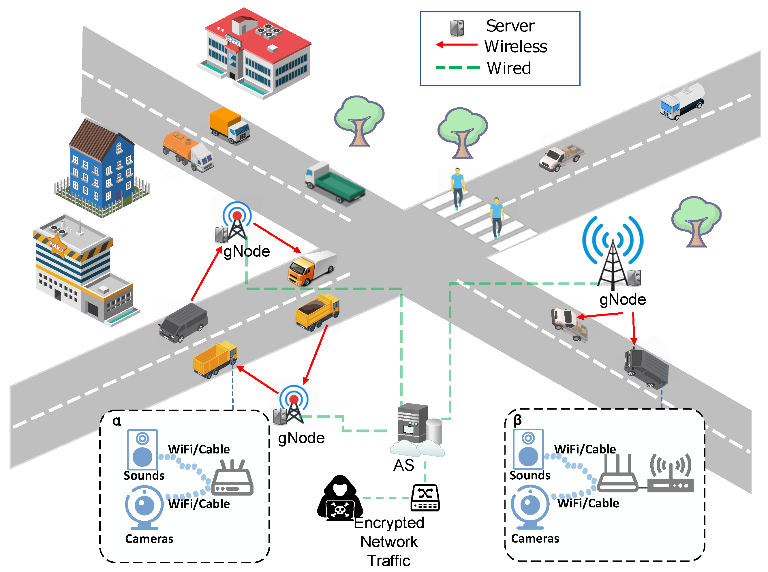
Nonetheless, several challenges arise in discerning multiple IoV devices in multi-level router environments. One challenge is the fluctuations in network features induced by wired or wireless transmission and router switching. For instance, these fluctuations in a typical IoV scenario are shown in Figure 1. In this figure, wired transmission means that IoV connects to the Telematics Box (T-BOX) via the bus, and wireless transmission means that IoV devices use 3G/4G to gNode. To alleviate this challenge, this paper sets up a simulation environment by applying router switching to collect relatively authentic traffic data. Then, a series of network graphs are constructed by leveraging GNN to effectively capture the relationships among complex flows and achieve improved identification performance. The main contributions of this paper are three-fold.

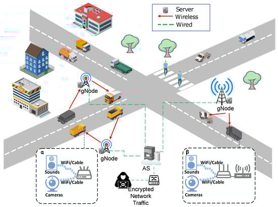
Figure 1. Packet change scenarios caused by route switching.

• We pose the problem of the poor generalization of IoV identified by most current flow identification models in packet change scenarios caused by route switching.
• We propose L-GraphSAGE, a GNN-based IoV application identification framework. L-GraphSAGE combines model learning techniques and can identify instances of existing classes that are not encountered during the training process.
• We implement a set of graph construction optimization methods for identifying IoV devices. These methods are further optimized using an embedding generation algorithm to achieve more accurate identification of IoV devices.

The rest of this paper is organized as follows. Our aims are introduced in Section 2. We introduce the workflow of L-GraphSAGE in Section 3. The evaluation and conclusion are presented in Section 4 and Section 5, respectively.

2. Motivation

As shown in Figure 1, there are a lot of IoV devices running in cars, and cars are networked, so there are data flows in cars that the adversary listens to. The adversary discussed in this paper captures network traffic on a wireless access point. Their goal is to identify network flows generated by various IoV devices. We define the network flow as a sequence of packets corresponding to socket-to-socket communication identified by the tuple (src.ip, src.port, dst.ip, dst.port, protocol).

The adversary can trace back all network flows to different devices according to their source addresses. However, the adversary cannot obtain the plaintext payload and destination features of the flows. Our assumptions match the real-world scenario, since IoV devices’ network flows are typically encrypted, and the adversary cannot access the plaintext.

For the same IoV devices that function via wired transmission or wireless transmission, the IPs of their flows and their payloads carried by network flows through different levels of routers are both different in various network areas. As we mentioned before, the existing models have limitations in the identification of multiple IoV devices in multi-level router scenarios, so they have the problem of poor identification generalization in the scenario of Figure 1. To better illustrate how the feature vectors change in $\alpha$ and $\beta$ network environments. We guarantee that only environments $\alpha$ and $\beta$ switch, and the other conditions remain unchanged. We apply the t-SNE [18] method to project high-dimensional feature vectors extracted by algorithm [8] into 2D vectors. Dahua data collected from $\alpha$ and $\beta$ environments are shown in Table 1. Hence, we can draw all the vectors in 2D space, which is shown in Figure 2. From these results, we can see that the distribution of feature vectors changes significantly when the network environment is changed. Therefore, traditional machine learning fails to correlate flow relationships, and traditional GNN first-order node aggregation information is missing, leading to misidentification according to Section 3.3.1. These results show the problem of poor identification generalization in Figure 1. To improve the generalization ability of identification applications, we developed L-GraphSAGE to identify untrained application flow. The model we developed improves the generalization of untrained data in complex scenarios by processing data features and enhancing node representation.

Table 1. Five IoT devices’ data collection.

IoV Device	Version	Functions	Collection Description	Server	Collection Time
Hikvision camera	B12HV3	Video real-time transmission	The device is connected by a switch to collect	Hikvision	5 h per scenario
Dahua camera	E6A	Video real-time transmission	The device is connected by WiFi to collect	Dahua	5 h per scenario
Wyze Cam	V3	Video real-time transmission	The camera is paired with WiFi via the Wyze APP, and PCAPdroid is used for collection	Wyze	5 h per scenario
Xiaomi Sound	Pro	Question and answer, timing, playing music, setting reminders	Data is collected by pairing WiFi	Xiaomi	5 h per scenario
Amazon Echo Dot	5th5	Question and answer	Data is collected by pairing WiFi	Amazon	5 h per scenario

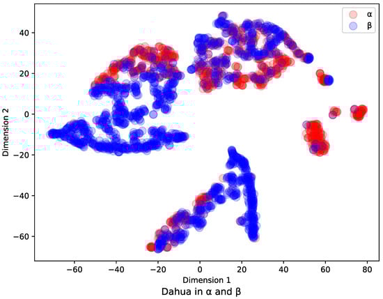
Figure 2. Distribution of feature vectors between $\alpha$ and $\beta$ environments. The t-SNE [18] method was used to project high-dimensional feature vectors extracted by algorithm [8] into 2D vectors. Dahua data collected from $\alpha$ and $\beta$ environments are shown in Table 1.

3. Workflow

3.1. Overview

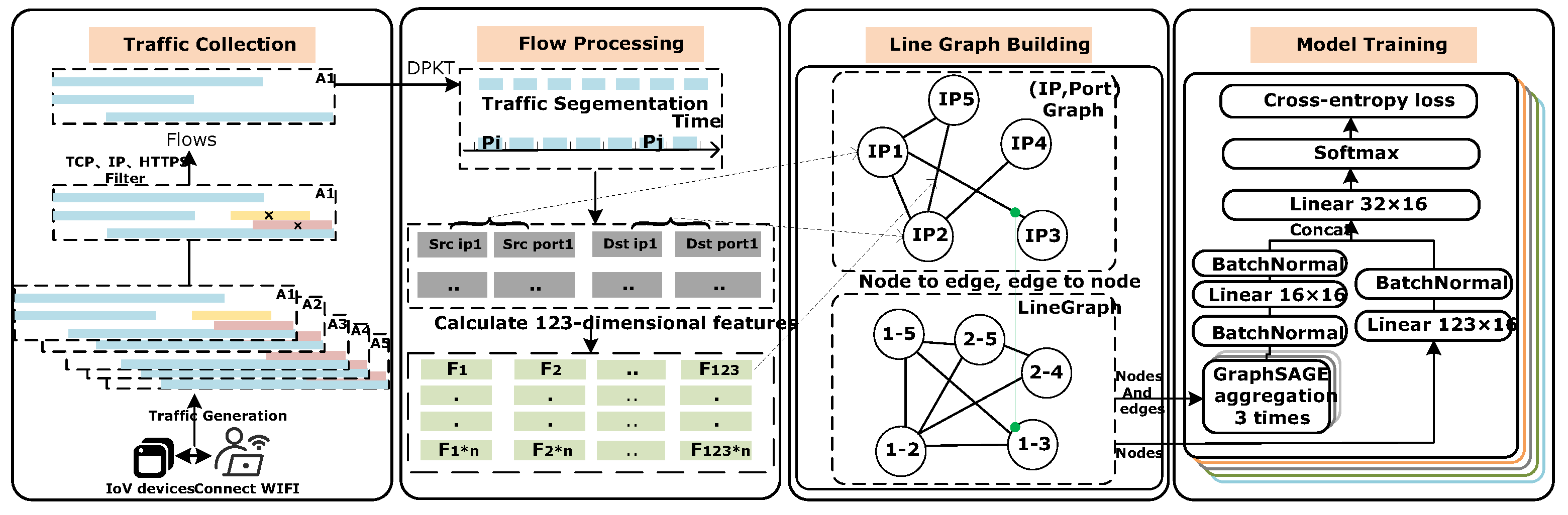
Figure 3 shows the system architecture, from which we can observe that the process of our work includes four phases: traffic collection, flow processing, line graph building, and model training.

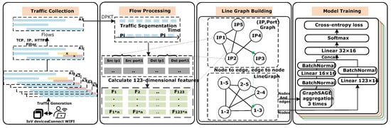
Figure 3. An overview of the L-GraphSAGE system architecture. For each IoV device, there are four phases. In the traffic collection phase, traffic collection and noise filtering are carried out. The flow processing phase uses DPKT to generate tuples and uses the algorithm in [8] to generate the tuple’s 123-dimensional features. The LineGraph building phase uses (IP, Port) as a node and edges as points to build the (IP, Port) graph, and then converts the points of the (IP, Port) graph to edges, and the edges to points, to build the line graph. In the model training phase, the constructed line graph is put into the model for training. Each of the five IoV device classes is trained on its model.

3.1.1. Traffic Collection

We establish an interactive environment to capture the traffic of real IoV devices, as shown in Figure 1. This involves connecting IoV devices to designated WiFi or cables, simulating traffic generated by various behaviors on these devices, and employing the Wireshark traffic collection tool on the host to monitor the forwarding port. Subsequently, we collect the generated traffic and store it in PCAP files. We eliminate most interference information by filtering out IP addresses and retaining PCAP packets containing strongly correlated traffic behavior data. Further details on this implementation are provided in Section 3.2.

3.1.2. Flow Processing

This module is responsible for the manual processing of pcap flow packets, including tasks such as flow segmentation, feature extraction, and feature generation. Flow segmentation cuts the pcap into different flows. DPKT is a Python module for fast, simple packet parsing, with definitions for the basic TCP/IP protocols. We use DPKT to extract flows from each pcap and divide flows by packets to obtain the tuple (timestamp, source IP, source port, destination IP, destination port, packet length), and remove timeout retransmission packets according to the sequence number. These tuples are then sorted by timestamp. All flows generated by the target application during this period are considered to be multiple samples. Feature extraction involves extracting size and arrival time features from each packet within the sample. Additionally, we apply the algorithm in [8] to generate 123-dimensional features.

3.1.3. Line Graph Building

Using the tuple (timestamp, source IP, source port, destination IP, destination port, packet length) generated during the flow processing phase, along with the tuple’s 123-dimensional features generated following the algorithm in [8], we build the (IP, Port) graph using tuple’s IP and Port as nodes and the tuple’s 123-dimensional features as edges. Then convert the (IP, Port) graph’s nodes to edges, and edges to nodes.

3.1.4. Model Training

The GNN is used to construct a relationship graph between flows. First, the processed data are stored as a two-dimensional array according to each row of tuples, features, and labels. Upon loading the data, the (IP, Port) is designated as the node, while the flow serves as the edge to construct an undirected graph with edge attributes. Through mapping relationships, the (IP, Port) of the original graph are converted into edges, and the edges are transformed into points to form a line graph. Second, the constructed line graph is fed into the GraphSAGE model for training. Batch normalization stabilizes training, and a linear layer is added to prevent gradient explosion. Softmax is utilized for data normalization, and the difference loss between relations is computed for all samples’ softmax vectors to optimize the adaptive process. The optimizer adopts Adam, while the loss function applies cross-entropy to measure the difference between the model output and the actual label. Finally, this loss function assumes that the model’s output is a probability distribution, and then calculates the deviation between the probability distribution of the model’s output and the probability distribution of the actual label.

3.1.5. Model Inference

The flow that needs to be identified is collected, and the subgraphs are constructed. These are then fed into different IoV graph models to obtain the maximum probability as the inference identification result.

3.2. Data Collection and Feature Processing

The data collection is divided into three stages: sender, collection, and data labeling. The sender is IoV devices in Table 1.

3.2.1. Sender

We pair audio speakers with routed WiFi and regularly set questions to audio speakers; thus, the audio speakers can answer questions regularly to generate traffic. As for cameras, we connect them directly to the router, enabling them to transmit real-time video data. To effectively simulate dynamic scenarios, we periodically switch the WiFi connection to change the IP address.

3.2.2. Collection and Data Labeling

To collect data traffic information from the speakers and cameras routed to the servers, we utilize a switch for channel detection. We filter the traffic by source IP addresses to generate PCAP files, which are then manually labeled for each batch.

3.3. L-GraphSAGE Algorithm

By transforming (IP, Port) into an edge and representing the flow as a node, a graph is constructed, where the edge connects nodes according to the association of the flow. This method makes full use of node features, such as attributes, node context, and node degree, for inductive learning. The main theoretical foundations and research methodologies encompass the following aspects:

3.3.1. Embedding Generation Algorithm

Hamilton et al. [19] proposed the GraphSAGE algorithm, which can generate vector representations of unknown nodes and has been widely applied in many fields. We utilized this algorithm and improved it, as shown in Algorithm 1.

Algorithm 1 assumes that the model has been trained and the parameters must be fixed. We assume that we have learned the parameters of K aggregator functions (expressed as $AD{D}_k$, $\forall k\in \{1,...,K\}$), which aggregate information from node neighbors, as well as a set of weight matrices $W^k$, $\forall k\in \{1,...,K\}$, which are used to propagate information between different layers of the model.

Algorithm 1: GraphSAGE embedding generation algorithm

Input: Graph G(V, E); input the tuple’s 123-dimensional features {$x_v$, $\forall v\in$ V}; normalized function STD; depth $K=3$; weight matrices $W^k$, $\forall k\in$ {1,...,K}; weight matrices $W^L$; non-linearity $\sigma$; aggregator functions $AD{D}_k$, $\forall k\in$ {1,..., K}; neighborhood function N: v → $2^v$    Output: Vector representations $z_v$ for all $v\in V$   1: $h_v^0\leftarrow STD\left(x_v\right)$, $\forall v\in$V   2: for $1\le k\le \left|K\right|$ do   3:   for $\forall v\in V$ do   4:    $h_{N\left(v\right)}^k\leftarrow AD{D}_k\left(\{h_u^{k-1},\forall u\in N\left(v\right)\}\right)$   5:    $h_v^k\leftarrow \sigma (W^k·CONCAT(h_v^{k-1},h_{N\left(v\right)}^k))$   6:   end for   7:   $h_v^k\leftarrow h_v^k/{\parallel h_v^k\parallel }_2,\forall v\in V$   8: end for   9: $z_v\leftarrow h_v^K,\forall v\in V$    10: $z_v\leftarrow W^L·z_v,\forall v\in V$    11: return $z_v,\forall v\in V$

Algorithm 1 describes the embedding generation process in a case where the entire graph G(V, E), and features for all nodes $x_v$ representing the tuple’s 123-dimensional features, $\forall v\in V$, are provided as inputs. We aggregated the features of neighbor nodes from the 1st to the nth order and found that setting $K=3$ yielded the best results, as discussed in Section 4.2. Each step in the outer loop of Algorithm 1 proceeds as follows, where k denotes the current step in the outer loop and $h^k$ denotes a node’s representation at this step: First, each node $v\in V$ aggregates the representations of the nodes in its immediate neighborhood, $\{h_u^{k-1},\forall u\in N\left(v\right)\}$, into a single vector $h_{N\left(v\right)}^k$. Note that this aggregation step depends on the representations generated at the previous iteration of the outer loop (i.e., $k-1$), and the $k=0$ (“base case”) representations are defined as the input node features. After aggregating the neighboring feature vectors, GraphSAGE then concatenates the node’s current representation, $h_v^{k-1}$, with the aggregated neighborhood vector, $h_{N\left(v\right)}^k$, and this concatenated vector is fed through a fully connected layer with the nonlinear activation function $\sigma$, which transforms the representations to be used at the next step of the algorithm (i.e., $h_v^k,\forall v\in V$). For notational convenience, we denote the final representation’s output at depth K as $z_v\equiv h_v^K,\forall v\in V$. The aggregation of the neighbor representations can be performed by a variety of aggregator architectures in Figure 3. $W^L$ represents the weight parameter of $h_v^K$ through three linear layers.

3.3.2. Aggregator

The vector of the current node and the vector of the adjacent node are summed in the corresponding dimension. The specific formula is (1), where W represents the weight parameter, $h_v^{k-1}$ represents the $k-1$ step representation of node v, $h_u^{k-1}$ represents the $k-1$ representation of v’s neighbor u, and $N\left(v\right)$ represents the first-order neighbor node of v.

$$\begin{array}{c}\hfill h_v^k\leftarrow \sigma (W·ADD\left(h_v^{k-1}\cup h_u^{k-1},\forall u\in N\left(v\right)\right))\end{array}$$

(1)

We can choose other aggregation functions, such as Mean, Max, or LSTM. The reason why we choose Add is explained in the ablation experiment section (Section 4.1).

3.3.3. Parameter Updating

Given that L-GraphSAGE outputs flows with associated labels, we selected the cross-entropy loss function to optimize our model. The specific formula is as follows (2):

$$\begin{array}{cc}\hfill & l(x,y)=-{\displaystyle \frac{1}{N}}\sum _{n=1}^N\sum _{c=1}^C{w}_c·log{\displaystyle \frac{exp\left(x_{n,c}\right)}{{\displaystyle \sum _{i=1}^C}exp\left(x_{n,i}\right)}}·y_{n,c}\hfill \end{array}$$

(2)

In the above Formula (2), x is the input, y is the target label, w is the weight value, and C is the number of classes. Additionally, N is the total number of flows. For this loss function, we expect the proportion of each class in the same class to be larger, and the loss to approach zero.

4. Evaluation

To verify the validity of the model, we evaluated the data on publicly available datasets (UNSW Sydney IoV datasets) and the dataset collected by ourselves.

4.1. Ablation Experiment

• Experimental setup. The environment used in our experiment was Intel(R) Xeon(R) CPU E5-2678 v3 @ 2.50GHz, CPU 48 cores, 2 threads per core, 2 GPU TITAN RTX, 64-bit Ubuntu 22.04.1LTS, x86_64. The network environment incorporated a combination of normal and UNSW Sydney IoV flows (Pixtar Photo Frame, TP-Link Camera, Triby Speaker, Withings Baby Monitor, Withings Sleep Sensor ) [20]. As mentioned above, there are many kinds of node aggregation methods in L-GraphSAGE, including Mean, Add, Max, and LSTM. In order to verify which aggregation function is the most effective, we conducted an ablation experiment using public datasets. The training ratio was 1:1:1:1:2. The inference ratio was 1:1:1:1:2. We ensured that the inference data did not appear in the training data. The training epochs were the same.
• Result. The experimental results are shown in Table 2, where five training and inference results are averaged. The experimental results show that the Add function is better in UNSW Sydney. Therefore, in the following experiment, we chose Add to aggregate node information. In particular, we find that LSTM outperforms the Add function because LSTM relies on temporal features, and the limited visibility of temporal features during graph construction can result in the suboptimal utilization of temporal information.
  Table 2. Aggregation on UNSW Sydney datasets.

  Aggregation Method	UNSW Sydney Datasets (Five IoT Devices)
  	Accuracy	Recall	F1-Score
  L-GraphSAGE-Mean	69.10%	63.18%	62.76%
  L-GraphSAGE-Add	94.23%	93.34%	94.02%
  L-GraphSAGE-Max	78.10%	77.92%	77.59%
  L-GraphSAGE-LSTM	85.67%	85.00%	85.48%

4.2. Evaluation on Public Datasets

• Experimental setup: In order to reflect the model effect in a more comprehensive way, Recall, Precision, F1-score, and Accuracy were used as metrics. We only identified Pixtar Photo Frame, TP-Link Camera, Triby Speaker, Withings Baby Monitor, and Withings Sleep Sensor. The reason we chose these five classes is that UNSW Sydney is real traffic on the Internet, which does not have a specific scenario. To reflect the model identification ability, the training ratio was 1:1:1:1:2 and the inference ratio was 1:1:1:1:2. We ensured that the inference data did not appear in the training data, and the training Epochs were the same. To stabilize the experimental data, the results of the five training and inference identifications were averaged.
• Results: The experimental results are shown in Table 3, from which we can observe that our method is powerful on the UNSW Sydney dataset since we effectively aggregate the relationship between flows. Compared with other models used on UNSW Sydney, the accuracy of our model on this dataset is improved by 0.23% and the F1 of our model on this dataset is improved by 3.02%. However, in the datasets, some flow features are not obvious and are too similar (tuples are the same and features are similar), leading to a lower Recall. As a consequence, each IoV-built graph neural network is disturbed. So compared with DLGNN, our model Recall is decreased by 0.36%. To highlight the advantages of L-GraphSAGE, we conducted the following analysis: dynamic line graph neural network (DLGNN) [21]-based identification with semisupervised learning. DLGNN only performs first-order neighbor node aggregation. L-GraphSAGE performs third-order neighbor node aggregation, which contains more node information. Recursive Feature Elimination with Random Forest (RFE-RF) [22] is used for feature selection, and then, random forest is used for classification, but the key feature information of the node will be lost. Recursive Feature Elimination with multilayer perceptron (RFE-MLP) [23] is a hybrid feature selection method tasked for multi-class network anomalies using a multilayer perceptron network. RFE-MLP will lose the key feature information of nodes. ExtraTreesClassifier (ETC) [24] has no special structural assumptions about the correlation between features and cannot handle complex relationships between data. E-GraphSAGE(EG) [17] performs second-order neighbor node aggregation, and some key node information will be lost.
  Table 3. Comparison Results on UNSW Sydney datasets.

  Method	UNSW Sydney Datasets (Five IoT Devices)
  	Accuracy	Recall	F1-Score
  DLGNN [21]	94.00%	93.70%	89.22%
  RFE-RF [22]	83.34%	82.23%	80.36%
  RFE-MLP [23]	88.33%	86.70%	86.40%
  ETC [24]	92.22%	91.13%	91.00%
  EG [17]	84.95%	88.15%	86.05%
  L-GraphSAGE	94.23%	93.34%	94.02%

4.3. Evaluation on Packet Change Scenarios Caused by Route Switching

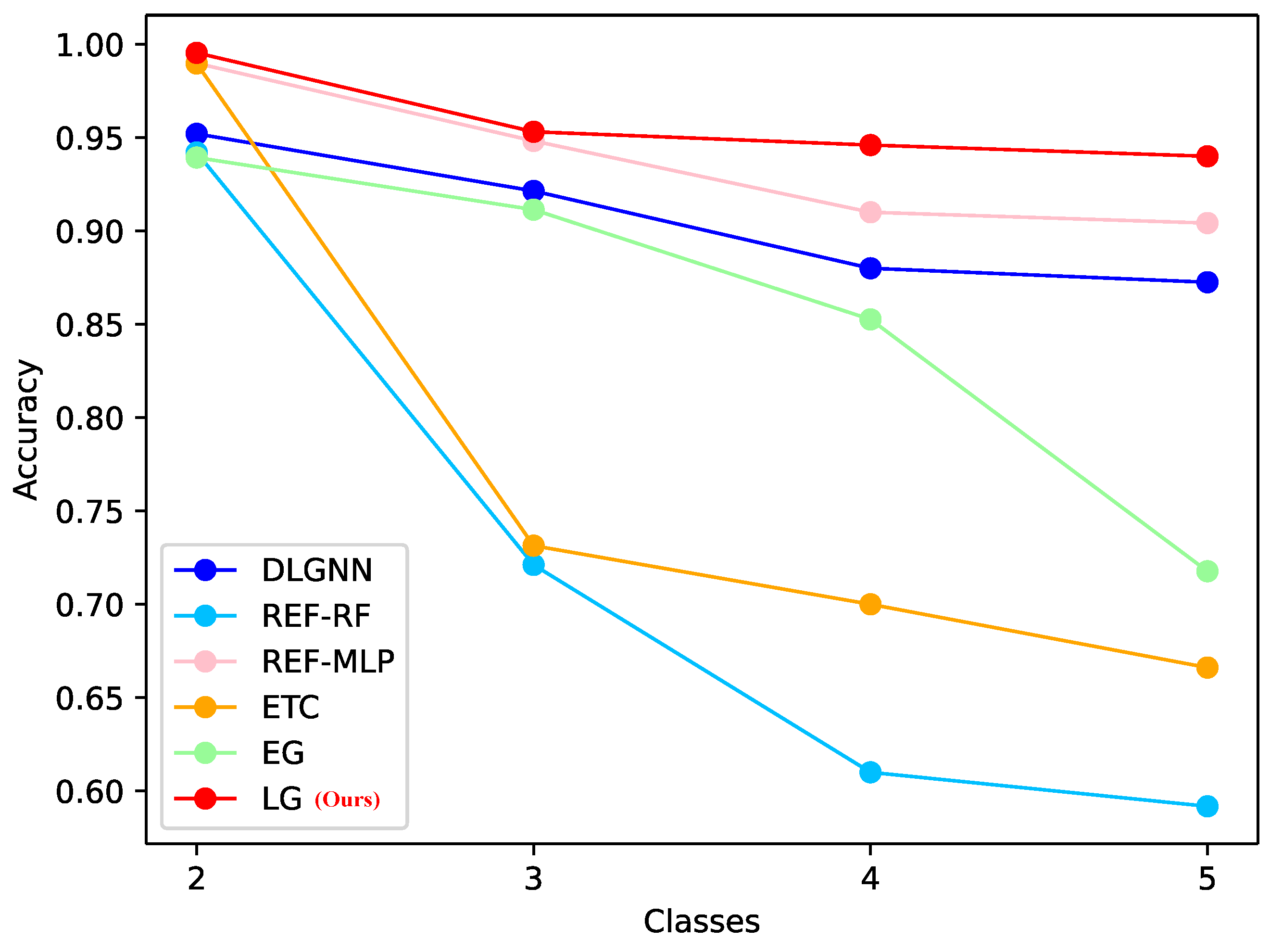
• Experimental setup: The scenario construction is shown in Figure 1. We used WiFi or Cable to connect the routers and collect IoV device traffic in environments $\alpha$ and $\beta$ through switches. Since most IoV devices communicate with different servers in reality, to simulate IoV applications more realistically, we utilize five IoV devices to communicate with different servers. The device list is shown in Table 1. For the Hikvision camera, we used switches to collect data. We simulated different environments by modifying the IP settings. For the Dahua camera, we used WiFi to collect data. We changed the environment by modifying the WiFi for the Dahua camera. For Wyze Cam, we paired it with WiFi via the Wyze APP, and PCAPdroid was used for collection. The process for Xiaomi and Amazon Sound was the same as that for Dahua. After that, we process the collected pcaps as described in Section 3.1.2. In fact, routers themselves generate traffic. Through our analysis, we found that the routers’ own packets only account for 4% of the total packets. We found that most of the routers are short flows, so we can use DPKT to filter them. To eliminate the noise effect, we filtered the non-functional flows of IoV devices to ensure that no other noise occurred. To evaluate the effect of the model, we used the data collected in the $\alpha$ or $\beta$ environment as the training set and the data collected in the $\alpha$ and $\beta$ environments as the inference set. We also used the Accuracy, Recall, and F1-score metrics for evaluation, and the results are shown in Table 4. To reflect the difference in environment transformation, we used $\alpha$ for training and the infer results from $\alpha$ and $\beta$ for comparison; then, we used $\beta$ for training and the infer results from $\alpha$ and $\beta$ for comparison. Additionally, we collect data from the $\alpha$ and $\beta$ environments and added classes. We ensured that the inference data did not appear in the training data. To stabilize the experimental data, the results of the five training and inference identifications were averaged. We conducted a visualization of the effect of model recognition ability when class increases in Figure 4 to verify the effect of class increase on the model.
  Table 4. Comparison results on five IoV devices’ datasets ($\alpha$ and $\beta$).

  Method	$\mathit{\alpha }$ Train, $\mathit{\alpha }$ Infer			$\mathit{\alpha }$ Train, $\mathit{\beta }$ Infer
  	Accuracy	Recall	F1-Score	Accuracy	Recall	F1-Score
  DLGNN [21]	96.06%	94.55%	94.92%	87.25%(↓8.8%)	87.25%(↓7.3%)	88.44%(↓6.5%)
  RFE-RF [22]	16.52%	21.80%	8.15%	59.18%(↑42.7%)	59.18%(↑37.4%)	48.99%(↑40.8%)
  RFE-MLP [23]	82.12%	85.73%	79.85%	90.42%(↑8.3%)	90.42%(↑4.7%)	91.38%(↑11.5%)
  ETC [24]	47.85%	64.18%	46.15%	66.61%(↑18.8%)	66.61%(↑2.4%)	55.22%(↑9.1%)
  EG [17]	90.02%	91.13%	88.26%	71.77%(↓18.3%)	71.77%(↓19.4%)	72.41%(↓15.9%)
  L-GraphSAGE	96.22%	96.22%	94.01%	94.00%(↓2.2%)	94.00%(↓2.2%)	94.17%(↑0.2%)
  Method	$\mathit{\beta }$ Train, $\mathit{\beta }$ Infer			$\mathit{\beta }$ Train, $\mathit{\alpha }$ Infer
  	Accuracy	Recall	F1-Score	Accuracy	Recall	F1-Score
  DLGNN [21]	94.42%	94.42%	94.03%	91.60%(↓2.8%)	91.60%(↓2.8%)	91.68%(↓2.4%)
  RFE-RF [22]	76.00%	76.00%	63.00%	76.00%(↑0%)	72.00%(↓4%)	73.00%(↑10%)
  RFE-MLP [23]	83.21%	83.21%	85.26%	68.70%(↓14.5%)	72.00%(↓13.2%)	74.19%(↓11.1%)
  ETC [24]	80.92%	80.92%	79.76%	60.31%(↓20.6%)	32.00%(↓48.9%)	22.28%(↓57.5%)
  EG [17]	91.22%	91.22%	91.71%	88.55%(↓2.7%)	88.55%(↓2.7%)	88.18%(↓3.5%)
  L-GraphSAGE	94.66%	94.66%	94.28%	93.60%(↓1.1%)	93.60%(↓1.1%)	93.65%(↓0.6%)

  

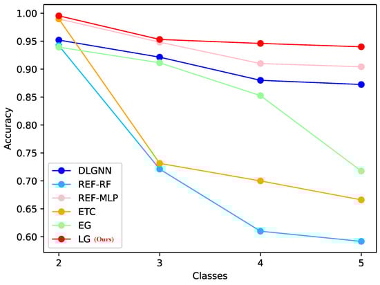  Figure 4. Model generalization on five IoV devices’ data collection.
• Results: The experimental results in Table 4 show that L-GraphSAGE has a good ability to identify IoV devices in complex scenarios. Although RFE-RF was trained in $\beta$, and its inference accuracy changed to 0% in $\alpha$ and $\beta$, its Recall and F1-score changed greatly. Compared with L-GraphSAGE’s training and inference results in the same environment, L-GraphSAGE’s training and inference in different environments are more stable. These experiments demonstrated that despite significant variations in the data collected by IoV in different environments and the utilization of different servers for communication, the L-GraphSAGE method can achieve better identification of IoV applications by utilizing (IP, Port) information. For other comparison models, there is no strict correlation between flows, resulting in the loss of a strong relationship between the flows. As a consequence, recognition in the real world is not as good as the method we proposed. As the number of classes increases, although the recognition accuracy of the L-GraphSAGE model decreases, it exhibits more stability than other models. Nevertheless, overfitting and underfitting occurred in this experiment. Some studies [25,26,27] require large amounts of training data to avoid overfitting and underfitting. Therefore, we increased the amount of training data from 1G pcap to 2G pcap for each IoV graph to avoid overfitting and underfitting. Moreover, we applied dropout and batch normalization during both the training and inference phases to mitigate overfitting and improve model generalization.

5. Conclusions

In this paper, we mitigated the issue of poor generalization observed in current flow identification models within diverse IoV communication scenarios involving various applications and servers. Specifically, we propose a GNN-based model named L-GraphSAGE to improve the generalization ability of model identification. Our model demonstrates promising performance on public datasets. Furthermore, we validate the effectiveness of multi-classification using the L-GraphSAGE model on datasets collected in our constructed scenarios. Our model achieves an F1 change rate of 0.20%(↑96.92%) in $\alpha$ train, $\beta$ infer and 0.60%(↑75.00%) in $\beta$ train, $\alpha$ infer. Considering that route switching results in IP conversion, we use L-GraphSAGE in this project to train the automatically collected data once a day. In anticipation of the inevitable presence of noise in real-world applications, our future research will focus on integrating controlled noise into the L-GraphSAGE model. This approach is aimed at evaluating and improving L-GraphSAGE’s robustness, ensuring that the proposed model performs reliably under non-ideal conditions.

References

- Laghari, A.A.; Khan, A.A.; Alkanhel, R.; Elmannai, H.; Bourouis, S. Lightweight-biov: Blockchain distributed ledger technology (bdlt) for internet of vehicles (iovs). Electronics 2023, 12, 677. [Google Scholar] [CrossRef]
- Chen, J.; Wang, Z.; Srivastava, G.; Alghamdi, T.A.; Khan, F.; Kumari, S.; Xiong, H. Industrial blockchain threshold signatures in federated learning for unified space-air-ground-sea model training. J. Ind. Inf. Integr. 2024, 39, 100593. [Google Scholar] [CrossRef]
- Taslimasa, H.; Dadkhah, S.; Neto, E.C.P.; Xiong, P.; Ray, S.; Ghorbani, A.A. Security issues in Internet of Vehicles (IoV): A comprehensive survey. Internet Things 2023, 22, 100809. [Google Scholar] [CrossRef]
- Chen, J.; Yan, H.; Liu, Z.; Zhang, M.; Xiong, H.; Yu, S. When Federated Learning Meets Privacy-Preserving Computation. ACM Comput. Surv. 2024, 56, 319. [Google Scholar] [CrossRef]
- Salman, O.; Elhajj, I.H.; Chehab, A.; Kayssi, A. A machine learning based framework for IoT device identification and abnormal traffic detection. Trans. Emerg. Telecommun. Technol. 2022, 33, e3743. [Google Scholar] [CrossRef]
- Fu, C.; Li, Q.; Shen, M.; Xu, K. Realtime robust malicious flow detection via frequency domain analysis. In Proceedings of the CCS ’21: Proceedings of the 2021 ACM SIGSAC Conference on Computer and Communications Security, Virtual, 15–19 November 2021; pp. 3431–3446. [Google Scholar]
- Zhu, K.; Hu, X.; Wang, J.; Xie, X.; Yang, G. Improving Generalization of Adversarial Training via Robust Critical Fine-Tuning. arXiv 2023, arXiv:2308.02533. [Google Scholar]
- Li, J.; Zhou, H.; Wu, S.; Luo, X.; Wang, T.; Zhan, X.; Ma, X. FOAP: Fine-Grained Open-World android app fingerprinting. In 31st USENIX Security Symposium (USENIX Security 22); USENIX Association: Boston, MA, USA, 2022. [Google Scholar]
- Bovenzi, G.; Di Monda, D.; Montieri, A.; Persico, V.; Pescapé, A. Few Shot Learning Approaches for Classifying Rare Mobile-App Encrypted flow Samples. In Proceedings of the IEEE INFOCOM 2023—IEEE Conference on Computer Communications Workshops (INFOCOM WKSHPS), Hoboken, NJ, USA, 20–20 May 2023. [Google Scholar]
- Al-Garadi, M.A.; Mohamed, A.; Al-Ali, A.K.; Du, X.; Ali, I.; Guizani, M. A survey of machine and deep learning methods for internet of things (IoT) security. IEEE Commun. Surv. Tutorials 2018, 22, 1646–1685. [Google Scholar] [CrossRef]
- Aleesa, A.M.; Zaidan, B.B.; Zaidan, A.A.; Sahar, N.M. Review of Intrusion Detection Systems Based on Deep Learning Techniques: Coherent Taxonomy, Challenges, Motivations, Recommendations, Substantial Analysis and Future Directions. Neural Comput. Appl. 2019, 32, 9827–9858. [Google Scholar] [CrossRef]
- Apruzzese, G.; Colajanni, M.; Ferretti, L.; Guido, A.; Marchetti, M. On the effectiveness of machine and deep learning for cyber security. In Proceedings of the Proceedings of 2018 10th International Conference on Cyber Conflict (CyCon), Tallinn, Estonia, 29 May–1 June 2018; IEEE: Piscataway, NJ, USA, 2018; pp. 371–390. [Google Scholar]
- Berman, D.S.; Buczak, A.L.; Chavis, J.S.; Corbett, C.L. A survey of deep learning methods for cyber security. Information 2019, 10, 122. [Google Scholar] [CrossRef]
- Ferrag, M.A.; Maglaras, L.; Moschoyiannis, S.; Janicke, H. Deep learning for cyber security intrusion detection: Approaches, datasets, and comparative study. J. Inf. Secur. Appl. 2020, 50, 102419. [Google Scholar] [CrossRef]
- Wickramasinghe, C.S.; Marino, D.L.; Amarasinghe, K.; Manic, M. Generalization of deep learning for cyber-physical system security: A survey. In Proceedings of the IECON 2018-44th Annual Conference of the IEEE Industrial Electronics Society, Washington, DC, USA, 21–23 October 2018; IEEE: Piscataway, NJ, USA, 2018; pp. 745–751. [Google Scholar]
- Xin, Y.; Kong, L.; Liu, Z.; Chen, Y.; Li, Y.; Zhu, H.; Gao, M.; Hou, H.; Wang, C. Machine learning and deep learning methods for cybersecurity. IEEE Access 2018, 6, 35365–35381. [Google Scholar] [CrossRef]
- Lo, W.W.; Layeghy, S.; Sarhan, M.; Gallagher, M.; Portmann, M. E-graphsage: A graph neural network based intrusion detection system for IoT. In Proceedings of the NOMS 2022-2022 IEEE/IFIP Network Operations and Management Symposium, Budapest, Hungary, 25–29 April 2022; pp. 1–9. [Google Scholar] [CrossRef]
- Hinton, G.; Van Der Maaten, L. Visualizing data using t-sne. J. Mach. Learn. Res. 2008, 9, 2579–2605. [Google Scholar]
- Hamilton, W.; Ying, Z.; Leskovec, J. Inductive representation learning on large graphs. Adv. Neural Inf. Process. Syst. 2017, 30, 1024–1034. [Google Scholar]
- Wannigama, S.; Sivanathan, A.; Hamza, A.; Gharakheili, H.H. Unveiling Behavioral Transparency of Protocols Communicated by IoT Networked Assets. In Proceedings of the IEEE WoWMoM workshop on Smart Computing for Smart Cities (SC2), Perth, Australia, 4–7 June 2024. [Google Scholar]
- Duan, G.; Lv, H.; Wang, H.; Feng, G. Application of a dynamic line graph neural network for intrusion detec tion with semisupervised learning. IEEE Trans. Inf. Forensics Secur. 2022, 18, 699–714. [Google Scholar] [CrossRef]
- Tonni, Z.A.; Mazumder, R. A novel feature selection technique for intrusion detection system using rf-rfe and bio-inspired optimization. In Proceedings of the 2023 57th Annual Conference on Information Sciences and Systems (CISS), Baltimore, MD, USA, 22–24 March 2023; pp. 1–6. [Google Scholar]
- Yin, Y.; Jang-Jaccard, J.; Xu, W.; Singh, A.; Zhu, J.; Sabrina, F.; Kwak, J. Igrf-rfe: A hybrid feature selection method for mlp-based network intrusion detection on unsw-nb15 dataset. J. Big Data 2023, 10, 15. [Google Scholar] [CrossRef]
- Sarhan, M.; Layeghy, S.; Moustafa, N.; Portmann, M. Netflow datasets for machine learning-based network intrusion detection systems. In Proceedings of the In Big Data Technologies and Applications: 10th EAI International Conference, BDTA, Virtual, 11 December 2020. [Google Scholar]
- Aceto, G.; Ciuonzo, D.; Montieri, A.; Pescapè, A. Mimetic: Mobile encrypted traffic classification using multimodal deep learning. Comput. Netw. 2019, 165, 106944. [Google Scholar] [CrossRef]
- Sirinam, P.; Imani, M.; Juarez, M.; Wright, M. Deep fingerprinting: Undermining website fingerprinting defenses with deep learning. In Proceedings of the 2018 ACM SIGSAC Conference on Computer and Communications Security, Toronto, ON, Canada, 15–19 October 2018. [Google Scholar]
- Sirinam, P.; Mathews, N.; Rahman, M.S.; Wright, M. Triplet fingerprinting: More practical and portable website fingerprinting with n-shot learning. In Proceedings of the 2019 ACM SIGSAC Conference on Computer and Communications Security, London UK, 11–15 November 2019. [Google Scholar]
Disclaimer/Publisher’s Note: The statements, opinions and data contained in all publications are solely those of the individual author(s) and contributor(s) and not of MDPI and/or the editor(s). MDPI and/or the editor(s) disclaim responsibility for any injury to people or property resulting from any ideas, methods, instructions or products referred to in the content. |
© 2024 by the authors. Licensee MDPI, Basel, Switzerland. This article is an open access article distributed under the terms and conditions of the Creative Commons Attribution (CC BY) license (https://creativecommons.org/licenses/by/4.0/).