Article

Small-Signal Modeling of Grid-Forming Wind Turbines in Active Power and DC Voltage Control Timescale

1
State Grid Hubei Electric Power Research Institute, Wuhan 430077, China
2
State Grid Hubei Electric Power Co., Ltd., Wuhan 430077, China
3
College of Information Science and Engineering, Wuhan University of Science and Technology, Wuhan 430081, China
*
Author to whom correspondence should be addressed.
These authors contributed equally to this work.
Electronics 2024, 13(23), 4728; https://doi.org/10.3390/electronics13234728
Submission received: 8 October 2024 / Revised: 7 November 2024 / Accepted: 14 November 2024 / Published: 29 November 2024

Abstract

:
Grid-forming wind turbines (GFM-WTs) based on virtual synchronous control can support the voltage and frequency of power system by emulating the synchronous generator. The dynamic characteristics of a GFM-WT decided by virtual synchronous control, dq-axis voltage, and current control is significant for small-signal stability analysis. This paper builds a small-signal model of a GFM-WT in active power control (APC) and DC voltage control (DVC) timescale from the perspective of internal voltage. The proposed model describes how the magnitude and phase of the internal voltage are excited by the unbalanced active and reactive power when small disturbances occur. Interactions in different control loops can be identified by the reduced order model. We verify the accuracy of the proposed model in APC and DVC timescales by time domain simulations based on MATLAB/Simulink. Case studies show how the control parameters interact with each other in the two timescales.

1. Introduction

Grid-connected voltage source converters (VSCs) of WTs are essential equipment of the modern power system [1,2,3]. Depending on the type of grid-connected VSCs’ control, WTs are divided into two types: grid-following wind turbines (GFL-WTs) and GFM-WTs. A GFL-WT tracks the phase of terminal voltage using phase-locked loop (PLL) [4]. On the other hand, a GFM-WT generates a synchronous phase using the virtual synchronous control by detecting the grid frequency and voltage. In this way, a GFM-WT can be considered a controllable voltage source, which directly controls the phase and magnitude of its internal voltage [5]. The dynamic stability of GFM-WTs is a significant issue and has attracted extensive attention from researchers.
Using dynamic stability analysis, researchers have proposed different types of small-signal models of GFM-WTs. The state-space model of a GFM-WT was built considering the dynamics of each element in [6]. Baruwa, M. et al. proposed a state-space model to analyze low-frequency oscillation related to GFM-WTs [7]. Models of a GFM-WT with distributed virtual inertia were derived in weak-grid conditions [8,9]. On the basis of the proposed state-space models, eigenvalue and singular value decomposition analysis can evaluate the small-signal stability of the systems. However, the order of the state-space models considering full timescales is too high, which causes difficulties for the stability analysis of a system with multiple GFM-WTs.
Impedance-based models are proposed to describe the dynamic characteristics of a GFM-WT. The wideband dq-frame impedance-based models of GFM-WTs are established with inner voltage and current control loops [10,11,12]. A sequence impedance model of a GFM-WT based on harmonic linearization is established [13]. Based on Nyquist stability criterion or generalized Nyquist criterion, one can determine the stability of a system with GFM-WTs utilizing the proposed impedance-based models.
In order to describe the dynamic characteristics with mechanism understanding, some researchers have proposed small-signal models of VSCs in a type-4 wind turbine [14,15,16] and a multi-terminal HVDC system [17,18] based on the motion equation concept. Y. Huang et al. proposed the concept of stability in the DVC timescale and described the dynamic characteristics of the DC voltage of VSCs by equivalent damping [15,16]. The results showed that the stability of VSCs in the DVC timescale is very important for renewable energy systems. Furthermore, H. Yuan, W. Zheng et al. described the characteristics of VSCs of a type-4 wind turbine and a multi-terminal HVDC system in a DVC timescale with active/reactive power and phase/magnitude of internal voltage as the interfaces [17,18]. The models can characterize the dynamics of VSCs in DVC timescale with clear mechanism understanding, i.e., equivalent inertia and damping. However, for GFM-WTs, it lacks a small-signal model considering both virtual synchronous control in APC timescale and control loops in the DVC timescale.
This paper builds a small-signal model of a GFM-WT from the perspective of internal voltage in APC and DVC timescales. In this model, the active and reactive power are the input signals and the phase and magnitude of the internal voltage are the output signals. The dynamics of a GFM-WT is characterized by the corresponding transfer functions from the active/reactive power to the phase/magnitude of the internal voltage. The coupling of a GFM-WT from the reactive/active power to the phase/magnitude is also described analytically. Moreover, we analyze the interactions among the control parameters in the APC timescale and parameters in the DVC timescale.
The structure of this paper is as follows: Section 2 introduces the basic control scheme of a GFM-WT and the concept of internal voltage. Section 3 builds the original small-signal model with a GFM-WT in APC and DVC joint timescale. Model verification and case studies are presented in Section 4 and Section 5, conclusions are drawn in Section 6.

2. Control Scheme and Definition of Internal Voltage

This section introduces the basic control scheme of a GFM-WT connected in an infinite grid and presents the concept of internal voltage.

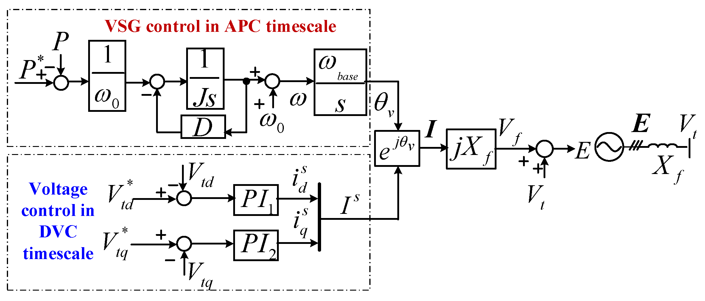
2.1. Basic Control Scheme of a GFM-WT

Figure 1 depicts the basic control scheme of a GFM-WT, including VSG control, voltage outer loop, and current inter loop. To eliminate the current harmonics, a GFM-WT is connected to the grid via an LC filter. The effect of a filter capacitor C f and the dynamics of the inductance currents are neglected.
The control process of a GFM-WT is as follows: At first, the active power and reactive power can be calculated by measuring the terminal voltage and current at the point of common coupling (PCC). Then, VSG control analogously the inertia and damping characteristics of the synchronous generation to obtain the virtual synchronous angle θ v . The dq axis reference voltages are aquired through the reactive power. In this paper, the reference voltage values are provided as 1 and 0. Next, voltage and current loops act sequentially to produce the dq-axis reference internal voltage by the PI control. The PWM modulation signal is obtained through dq transformation. The IGBT control signal is produced by a PWM controller. Consequently, the inverter generates voltage, which is characterized as its internal voltage E θ .
The response time of the VSG, voltage loop, and current loop is approximately 1 s, 0.1 s, and 0.01 s, respectively. For simplicity, only the APC and DVC timescales are considered, allowing currents to track their reference values instantaneously.

2.2. Definition of Internal Voltage

A grid-connected device can be represented by an equivalent voltage source in series with an impedance. Within the AC system, the equipment inputs and outputs both active and reactive power, while energy storage elements store unbalanced power [19,20]. The state expression for this unbalanced power is determined by the magnitude and phase of the internal voltage [21,22]. When the system is perturbed, the magnitude and phase of the internal voltage begin to change in response to variations in imbalance power, reflecting the dynamic characteristics of the equipment itself.
Hence, the phase and magnitude dynamic of the internal voltage under the excitation of active and reactive power can be used as a universal idea to describe the dynamic characteristics of equipment in the AC grid.

3. Proposed a GFM-WT Model

A GFM-WT model is proposed to analyze the dynamics of the internal voltage, which includes two parts: building the original small-signal model and simplifying it to obtain an analytical model represented by transfer functions.

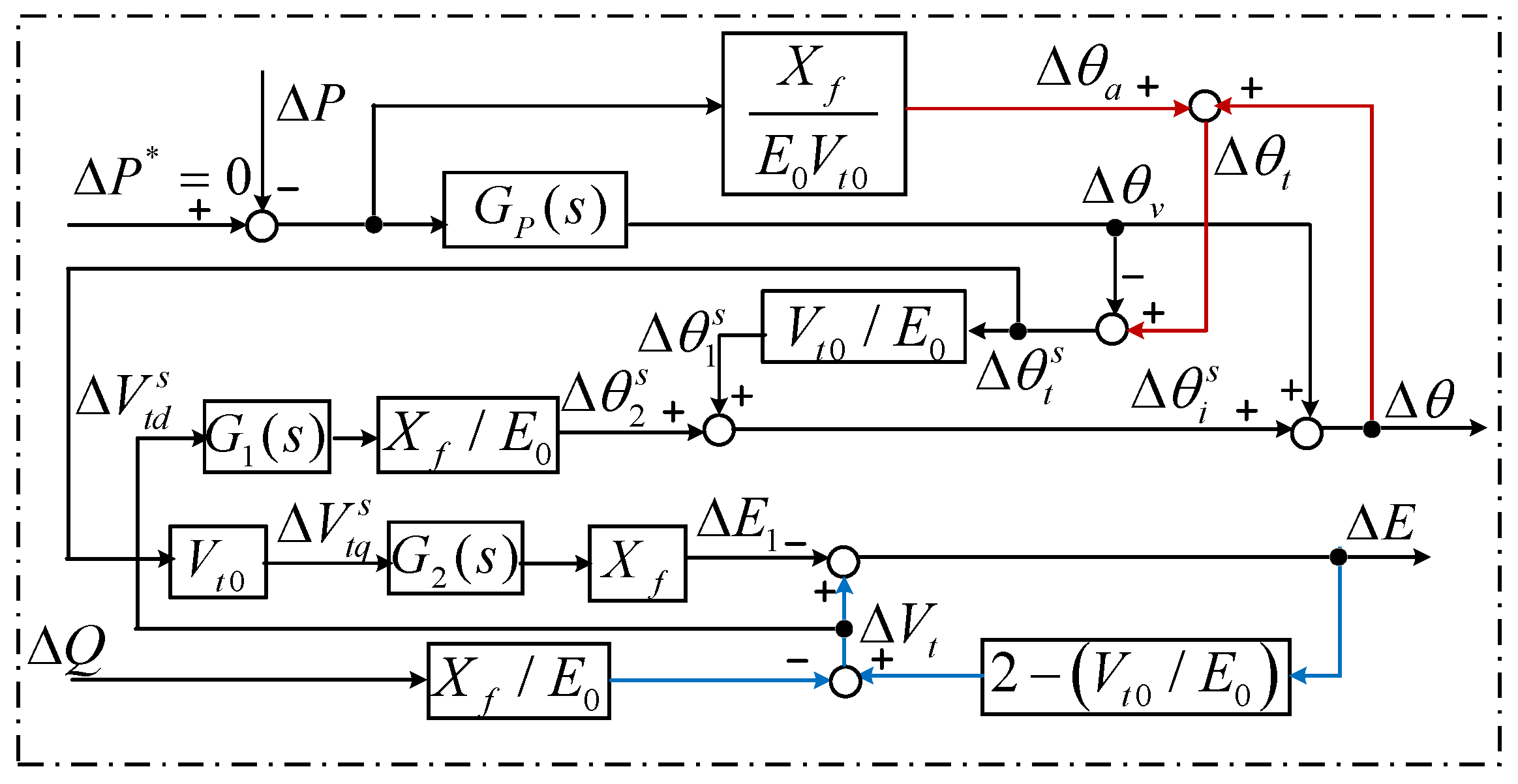
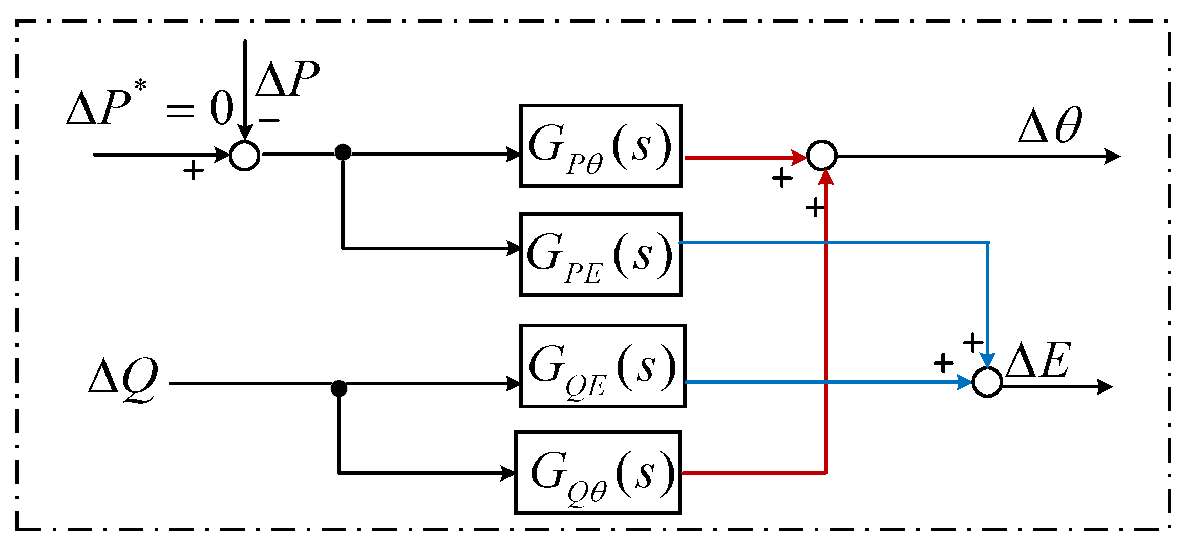
3.1. The Original Small-Signal Model of a GFM-WT

Based on the system control configuration and the assumptions in Section 2, Figure 2 illustrates the dynamics diagram of a GFM-WT in APC and DVC joint timescales. During this dynamic process, the VSG control yields a synchronization angle, and the voltage control loop outputs dq-axis reference currents. Utilizing the circuit relationships, the internal voltage is determined and considered as the final representation. The nonlinear differential-algebraic equations of the system can be linearized under small perturbations; hence, each control loop needs to be linearized at the initial operating point. The procedures are as follows:
(1) Linearization of active power control: Active power control can be depicted as
ω = P * P ω 0 1 J s + D + ω 0 ,
θ v = ω b a s e s ω 0 .
where ω 0 is rated angular frequency. Linearizing (1) and (2) at some initial operating points, presents
Δ ω = 1 J s + D Δ P ,
Δ θ v = ω b a s e s Δ ω .
Therefore, the phase of the virtual synchronous can be further expressed as
Δ θ v = ω b a s e J s 2 + D s Δ P G P ( s ) Δ P .
(2) Linearization of the production of the dq-axis terminal voltage: The dq components of terminal voltage can be expressed as
V t d s = V t c o s θ t s ,
V t q s = V t s i n θ t s ,
where θ t s is the angle of the terminal voltage in the VSG-synchronized frame, it can be indicated as
θ t s = θ t θ v .
where θ t is the angle of the terminal voltage in the public frame, Linearizing (6)–(8) at certain initial operating point yields
Δ V t d s = c o s θ t 0 s Δ V t V t 0 s i n θ t 0 s Δ θ t s ,
Δ V t q s = s i n θ t 0 s Δ V t + V t 0 c o s θ t 0 s Δ θ t s ,
Δ θ t s = Δ θ t Δ θ v .
(3) Linearization of dq-axis voltage loop control: The specific expressions of voltage loop are described as
i d s = V t d s * V t d s k P 1 + k I 1 s ,
i q s = V t q s * V t q s k P 2 + k I 2 s .
where k P 1 and k I 1 are the proportional and integral parameters of the PI controller in d-axis voltage controller, and k P 2 and k I 2 are proportional and integral parameters of the PI controller in q-axis voltage controller. Linearizing (12) and (13) at some initial operating point results
Δ i d s = k P 1 s + k I 1 s Δ V t d s G 1 ( s ) Δ V t d s ,
Δ i q s = k P 2 s + k I 2 s Δ V t q s G 2 ( s ) Δ V t q s .
(4) Linearization of the generation of the internal voltage: According to the Figure 2, the internal voltage can be expressed as
E = j X f i + V t .
In VSG-synchronized frame, the dq components of the internal voltage can be written as
E d s = V t c o s θ t s X f i q s ,
E q s = V t i s i n θ t s + X f i d s ,
Linearizing (17) and (18) at some initial operating point produces
Δ E d s = c o s θ t 0 s Δ V t V t 0 s i n θ t 0 s Δ θ t s X f Δ i q s .
Δ E q s = s i n θ t 0 s Δ V t + V t 0 c o s θ t 0 s Δ θ t s + X f Δ i d s .
On the other hand, the dq components of the internal voltage can be directly decomposed using the vector. The formulas for decomposition are
E d s = E c o s θ i s ,
E q s = E s i n θ i s ,
where θ i s is the angle of the internal voltage in the VSG-synchronized frame, and θ i s can be written as
θ i s = θ θ v .
where θ is the angle of the internal voltage in the public frame. Linearizing (21)–(23) at some initial operating point, we have
Δ E d s = c o s θ i 0 s Δ E E 0 s i n θ i 0 s Δ θ i s ,
Δ E q s = s i n θ i 0 s Δ E + E 0 c o s θ i 0 s Δ θ i s .
Δ θ i s = Δ θ + Δ θ v .
Combining (19)–(20) and (24)–(25), the magnitude and the phase of the internal voltage in the VSG-synchronized frame can be derived as
Δ θ i s = c o s θ i 0 s E i 0 X f Δ i d s + V t 0 Δ θ t s + s i n θ i 0 s E i 0 X f Δ i q s Δ V t ,
Δ E = c o s θ i 0 s X f Δ i q s + Δ V t + s i n θ i 0 s X f Δ i d s + V t 0 Δ θ t s .
Consequently, the original linearized model of a GFM-WT in APC and DVC joint timescales is obtained as shown in Figure 3.

3.2. Simplify the GF-WT Small-Signal Model

Observe that additional values are present in the input signals, and the correlation between the power and internal voltage has not yet been directly established. Consequently, we will simplify the original linearized model depicted in Figure 3.

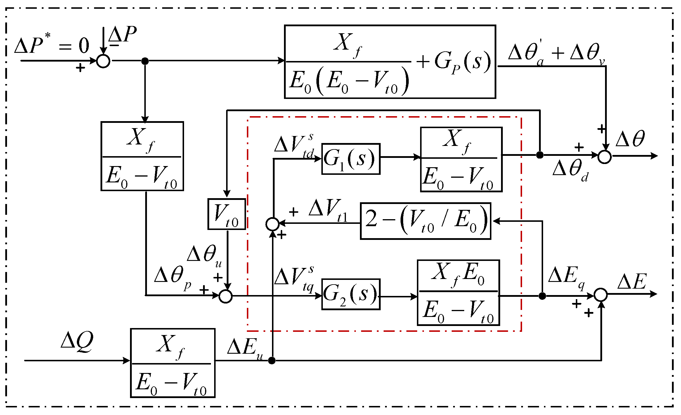
3.2.1. Replace the Terminal Voltage

The active and reactive power generated by the internal voltage and terminal voltage can be formulated as
P = E V t s i n θ i θ t X f ,
Q = E 2 X f E V t c o s θ i θ t X f .
Linearizing (29) and (30), Δ θ t and Δ V t are given as follows:
Δ θ t = Δ θ + 2 s i n θ i 0 s V t 0 Δ E X f c o s θ i 0 s E 0 V t 0 Δ P X f s i n θ i 0 s E 0 V t 0 Δ Q .
Δ V t = 2 c o s θ i 0 s V t 0 E 0 Δ E + X f s i n θ i 0 s E 0 Δ P X f c o s θ i 0 s E 0 Δ Q .
where θ i 0 s and θ t 0 s refer to the steady-state phase of the internal voltage and the terminal voltage in the VSG-synchronized reference frame, they are usually less than 10 degrees under small perturbations. That is, s i n θ i 0 s 0 , s i n θ t 0 s 0 , and c o s θ i 0 s 1 , c o s θ t 0 s 1 . Substituting the results into (31) and (32), Δ θ t and Δ V t can further be represented as
Δ θ t = Δ θ X f E 0 V t 0 Δ P .
Δ V t = 2 V t 0 E Δ E X f E i 0 Δ Q .
Hence, the original small-signal model depicted in Figure 3 can be changed into Figure 4 utilizing the above relationships.

3.2.2. Open the Feedback Loops

Figure 4 illustrates the presence of two feedback loops in the model. We initially simplify the feedback loop related to the phase of the internal voltage. The relationship among Δ θ , Δ θ 1 s , Δ θ 2 s and Δ θ v can be written as
Δ θ = Δ θ 1 s + Δ θ 2 s + Δ θ v
Substituting (5) into (35), Δ θ can be computed as
Δ θ = Δ θ 1 s + Δ θ 2 s G p ( s ) Δ P
Let us simplify the branch pertaining to Δ θ 1 s . We can establish the relationship among Δ θ 1 s , Δ θ t s , and Δ θ t as represented in Figure 4. The precise formulations are
Δ θ 1 s = Δ θ t s V t 0 E 0 ,
Δ θ t s = Δ θ t + G p ( s ) Δ P ,
Δ θ t = Δ θ X f E 0 V t 0 Δ P .
Substituting (39) into (38), Δ θ t s can be expressed as
Δ θ t s = Δ θ + ( G p ( s ) X f E 0 V t 0 ) Δ P
Combining (37) and (39), Δ θ 1 s can be computed as
Δ θ 1 s = V t 0 E 0 Δ θ X f E 0 2 Δ P + V t 0 E 0 G p ( s ) Δ P
The other branch involved Δ θ 2 s , can be described by Δ V t d s
Δ θ 2 s = X f E 0 2 G 1 ( s ) Δ V t d s
Substituting (41), (42) into (36), the phase of internal voltage can be calculated as
Δ θ = ( X f E 0 ( E 0 V t 0 ) + G p ( s ) ) Δ P + X f G 1 ( s ) ( E 0 V t 0 ) Δ V t d s
Substituting (43), into (40), the phase of internal voltage in VSG-synchronized reference frame can be presented as
Δ θ t s = X f V t 0 ( E 0 V t 0 ) Δ P + X f G 1 ( s ) ( E 0 V t 0 ) Δ V t d s
According to Δ V t q s = V t 0 Δ θ t s , the q-axis terminal voltage Δ V t q s can be further illustrated as
Δ V t q s = X f ( E 0 V t 0 ) Δ P + X f V t 0 G 1 ( s ) ( E 0 V t 0 ) Δ V t d s
In Figure 4, the feedback loop generated by the magnitude of the internal voltage Δ E can be depicted as
Δ E = Δ E 1 + Δ V t
where Δ E 1 can be described by Δ V t q s
Δ E 1 = G 2 ( s ) X f Δ V t q s
Substituting (47) and (34) into (46), Δ E can be given by
Δ E = X f E 0 V t 0 Δ Q + G 2 ( s ) X f E 0 E 0 V t 0 Δ V t q s
Substituting (48) into (34), in accordance with Δ V t d s = Δ V t , the d-axis terminal voltage Δ V t d s can be articulated as
Δ V t d s = G 2 ( s ) X f E 0 V t 0 ( 2 E 0 V t 0 ) Δ V t q s + X f E 0 V t 0 Δ Q
The new relationships among Δ θ , Δ E , Δ V t d s , Δ V t q s are given by (43), (45), (48) and (49). Figure 4 can now be converted into Figure 5.

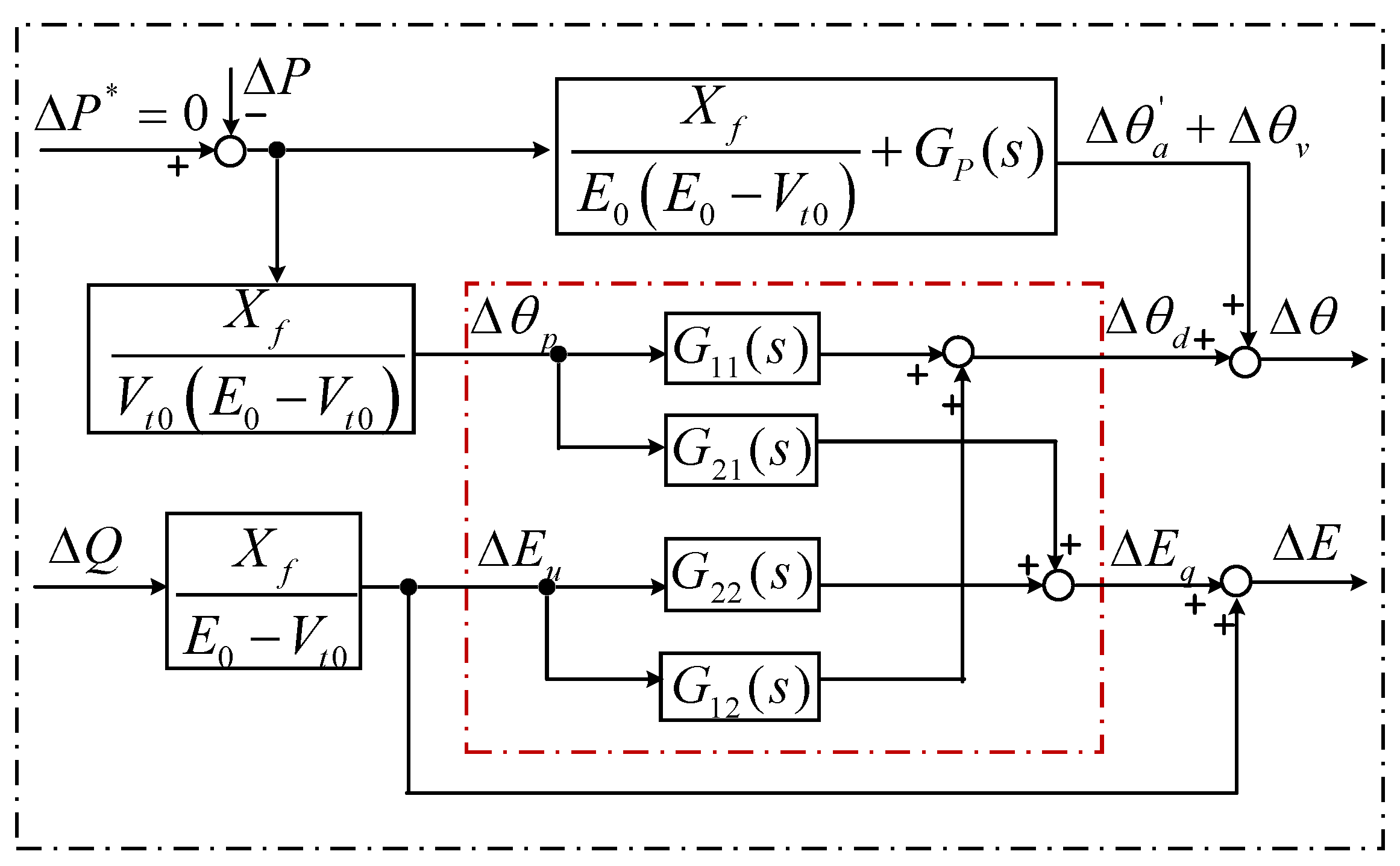
3.2.3. Simplify the Coupled Circuits

As manifested by the red dashed line in Figure 5, the subsequent mathematical relationships can be represented by the following five equations
Δ V t q s = Δ θ p + Δ θ u
Δ E q = G 2 ( s ) X f E 0 E 0 V t 0 Δ V t q s
Δ V t 1 = ( 2 V t 0 E 0 ) Δ E q
Δ V t d s = Δ V t 1 + Δ E u
Δ θ d = X f G 1 ( s ) E 0 V t 0 Δ V t d s
Combining (50)–(54), Δ θ d and Δ E q can be expressed by Δ θ p and Δ E u
Δ θ d = G 11 ( s ) Δ θ p + G 12 ( s ) Δ E u
Δ E q = G 21 ( s ) Δ θ p + G 22 ( s ) Δ E u
where the detailed expressions of G 11 ( s ) , G 12 ( s ) , G 21 ( s ) and G 22 ( s ) can be found in Appendix A.1. Figure 5 can be transformed into Figure 6.
Subsequently, by integrating with the remaining branches, the magnitude and phase of the internal voltage can be calculated by
Δ θ = ( X f E 0 ( E 0 V t 0 ) + G P ( s ) + X f G 11 ( s ) V t 0 ( E 0 V t 0 ) ) G P θ ( s ) Δ P + X f ( E 0 V t 0 ) G 12 ( s ) G Q θ Δ Q Δ E = X f V t 0 ( E 0 V t 0 ) G 21 ( s ) G P E ( s ) Δ P + X f ( E 0 V t 0 ) G 22 ( s ) G Q E ( s ) Δ Q
Figure 6 can now be modified to Figure 7. The correlation between the active/reactive power and the phase/magnitude of the internal voltage is articulated via transfer functions. Thus, the equations for amplitude and phase can be calculated in the presence of unbalanced power.

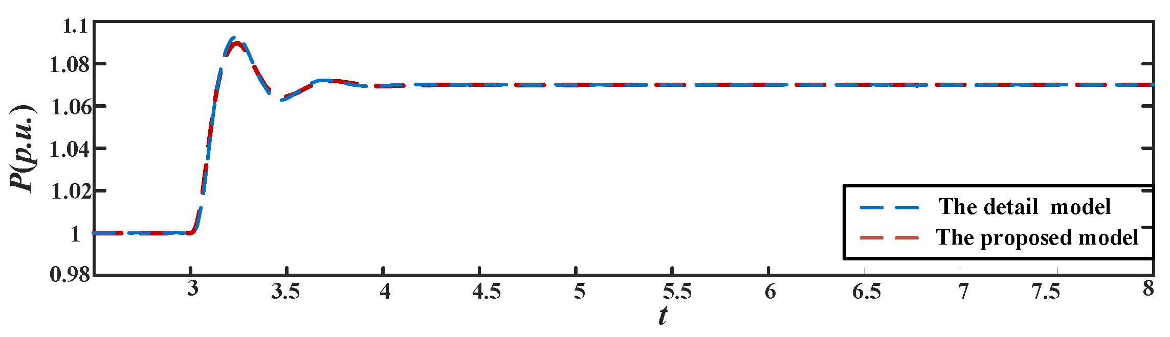
4. Verification of the Proposed GF-WT Model

The proposed model in the APC and DVC timescale is verified by comparing it with the detailed component model in MATLAB/Simulink. Assume that a small disturbance (0.01 p.u.) in active power occurs at 3 s. Figure 8 shows the responses of the active power output P of the proposed and detailed model under the parameters listed in Appendix A.2. The results indicate that the proposed model without the current loop can match the detailed model in the APC and DVC timescales. Table 1 presents the comparison results between the proposed and detailed models at different operating points, representing the closeness in values for λ 1 , 2 and λ 3 , 4 . Our focus is on λ 1 , 2 and λ 3 , 4 in the APC and DVC timescales, and consequently, the proposed model can be applied to analyze small-signal stability problems.

5. Case Study

In this section, several control parameters are selected to discuss the dynamic interactions at different timescales based on the proposed GFM-WT model. Other parameters are provided in Appendix A.2.

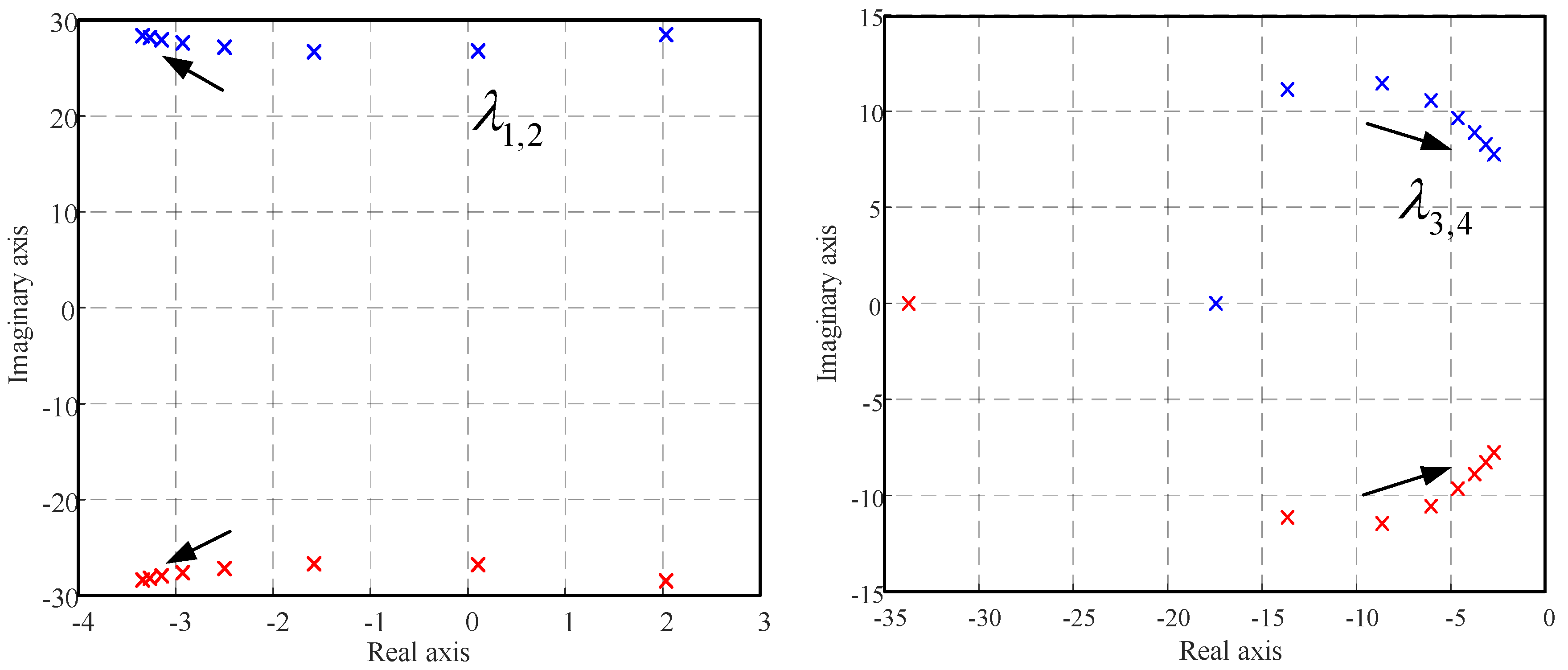
5.1. Effect of VSG Parameters

Considering the inertia coefficient J of the VSG control, with k I 1 = k I 2 = 100 , it is noted that the real parts of λ 1 , 2 transition from 2.00 to −3.34 as J increases, while the real parts of λ 3 , 4 change from −17.44 and −33.73 to −2.71, as indicated in Table 2. The damping ratio (DR) of λ 1 , 2 increases from 0 to 0.11, while that of λ 3 , 4 falls from 0.82 to 0.33. It may be concluded that J influences the APC and DVC timescales. The system is unstable at J = 2. Additionally, the root locus diagrams for λ 1 , 2 and λ 3 , 4 are shown in Figure 9.

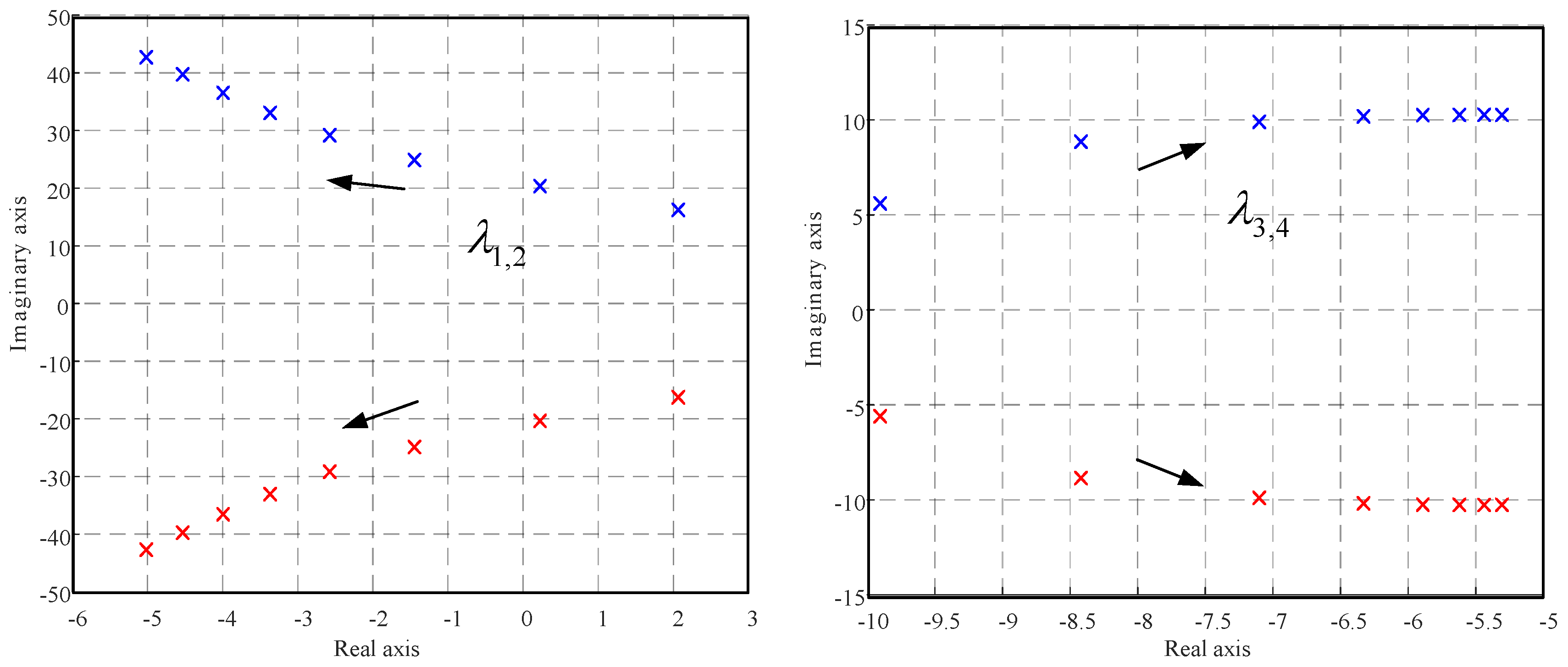
5.2. Effect of Voltage Control Parameters

Considering the integral parameter k I 1 with J = 8 , k I 2 = 140 , it is observed that the real parts of λ 1 , 2 transition from 2.06 to −5.01 as k I 1 increases, while those of λ 3 , 4 shift from −9.90 to −5.30, as shown in Table 3. The damping ratio (DR) of λ 1 , 2 rises from −0.09 to 0.11, whereas that of λ 3 , 4 declines from 0.57 to 0.45. This suggests that k I 1 significantly affects the APC and DVC timescales, with the system exhibiting instability at k I 1 = 50 . Furthermore, the root locus diagrams for λ 1 , 2 and λ 3 , 4 are demonstrated in Figure 10.
For the proposed GFM-WT model, it involves the APC and DVC timescale. The above effect of the parameters reveal the interactions between the APC and DVC timescale, thereby reflecting the dynamic stability in multiple timescales.

6. Conclusions

This paper builds a small-signal model of a GFM-WT in APC and DVC timescales from the perspective of internal voltage. The proposed model has the active and reactive power as the input signals and the phase and magnitude of the internal voltage as the output signals. Transfer functions among the active/reactive power and the phase/magnitude of the internal voltage can describe the characteristics and couplings in the APC and DVC timescale within the GFM-WT separately from the AC networks. Compared with the detailed component model, the proposed model is verified to be accurate in the DVC timescale. Moreover, the interactions among the controllers in the APC and DVC timescales are analyzed based on the model and verified by the simulations. In future work, we will further study how to describe the dynamics of a GFM-WT by equivalent inertia and damping based on the motion equation concept.

Author Contributions

Conceptualization, methodology, writing—reviewing and editing: K.J., X.J., D.L. and W.Z.; modeling, simulation: K.J., W.Z., L.T. and S.C.; All authors have read and agreed to the published version of the manuscript.

Funding

This study was supported by the State Grid Technology Project (NO.52153223001T) and the National Natural Science Foundation of China under Grant 62303356.

Data Availability Statement

Data are contained within the article.

Conflicts of Interest

Author Kezheng Jiang was employed by the State Grid Hubei Electric Power Research Institute. The remaining authors declare that the research was conducted in the absence of any commercial or financial relationships that could be construed as a potential conflict of interest.

Abbreviations

P , Q Active and reactive power output of GFM VSC
V t Terminal voltage vector
V t , θ t Magnitude and phase of the terminal voltage
E Internal voltage vector
E , θ Magnitude and phase of the internal voltage
V g Vector representation of the AC source
i , i Vector representation and the magnitude of AC current
θ v Output angle of the VSG control
X f , C f Filter reactance and capacitance of grid-side VSCs
X L Reactance of the AC transmission line
X g Reactance of the AC source
k P 1 , k I 1           Proportional and integral parameters of the PI controller in d-axis voltage controller
k P 2 , k I 2 Proportional and integral parameters of the PI controller in q-axis voltage controller
J , D Inertia and damping parameters of the VSG control
Subscripts:
d , q The subscripts represent the d-axis and q-axis components 
of the rotation coordinate system   
0The subscript represents the initial values in the steady-state condition
Superscripts:
*The subscript represents the reference value
sThe subscript represents the signals in VSG-synchronized reference frame

Appendix A

Appendix A.1

G 11 ( s ) = ( 2 E 0 V t 0 ) G 1 ( s ) G 2 ( s ) X f 2 V t 0 ( E 0 V t 0 ) 2 ( 2 E 0 V t 0 ) G 1 ( s ) G 2 ( s ) X f 2 V t 0
G 12 ( s ) = ( E 0 V t 0 ) G 1 ( s ) X f ( E 0 V t 0 ) 2 ( 2 E 0 V t 0 ) G 1 ( s ) G 2 ( s ) X f 2 V i 0
G 21 ( s ) = ( E 0 V t 0 ) G 2 ( s ) X f E 0 V t 0 ( E 0 V t 0 ) 2 ( 2 E 0 V t 0 ) G 1 ( s ) G 2 ( s ) X f 2 V t 0
G 22 ( s ) = G 1 ( s ) G 2 ( s ) X f 2 E 0 V t 0 ( E 0 V t 0 ) 2 ( 2 E 0 V t 0 ) G 1 ( s ) G 2 ( s ) X f 2 V t 0

Appendix A.2

  • (1) Steady-state reference values:
  • Inspecting power S b a s e = 45 , 000 VA, Impedance Z b a s e = 3.2089   Ω ,
  • Phase current    I b a s e = 96.4630 A, Frequency ω b a s e = 100 π rad/s,
  • Effective value of line voltage V b a s e = 380 V.
  • (2) Control parameters and operation points:
  • VSG control          D = 80
  • voltage loop control   k P 1 = k P 2 = 0.4 ,
  • operation points        P 0 = 1.02 p.u., U t 0 = U g 0 = 1 p.u., X f = 0.1 p.u., X g = 0.2 p.u.

References

  1. Chen, Z.; Guerrero, J.M.; Blaabjerg, F. A Review of the State of the Art of Power Electronics for Wind Turbines. IEEE Trans. Power Electron. 2009, 24, 1859–1875. [Google Scholar] [CrossRef]
  2. Blaabjerg, F.; Ma, K. Future on Power Electronics for Wind Turbine Systems. IEEE J. Emerg. Sel. Top. Power Electron. 2013, 1, 139–152. [Google Scholar] [CrossRef]
  3. Liu, P.; Xie, X.; Shair, J. Adaptive Hybrid Grid-Forming and Grid-Following Control of IBRs With Enhanced Small-Signal Stability Under Varying SCRs. IEEE Trans. Power Electron. 2024, 39, 6603–6607. [Google Scholar] [CrossRef]
  4. Yang, Y.; Li, C.; Cheng, L.; Gao, X.; Xu, J.; Blaabjerg, F. A Generic Power Compensation Control for Grid Forming Virtual Synchronous Generator With Damping Correction Loop. IEEE Trans. Ind. Electron. 2024, 71, 10908–10918. [Google Scholar] [CrossRef]
  5. Lasseter, R.H.; Chen, Z.; Pattabiraman, D. Grid-Forming Inverters: A Critical Asset for the Power Grid. IEEE J. Emerg. Sel. Top. Power Electron. 2020, 8, 925–935. [Google Scholar] [CrossRef]
  6. Hu, Y.; Shao, Y.; Yang, R.; Long, X.; Chen, G. A Configurable Virtual Impedance Method for Grid-Connected Virtual Synchronous Generator to Improve the Quality of Output Current. IEEE J. Emerg. Sel. Top. Power Electron. 2020, 8, 1477–1489. [Google Scholar] [CrossRef]
  7. Baruwa, M.; Fazeli, M. Impact of virtual synchronous machines on low-frequency oscillations in power systems. IEEE Trans. Power Syst. 2020, 36, 1934–1946. [Google Scholar] [CrossRef]
  8. Saeedian, M.; Sangrody, R.; Shahparasti, M.; Taheri, S.; Pouresmaeil, E. Grid—Following DVI—Based Converter Operating in Weak Grids for Enhancing Frequency Stability. IEEE Trans. Power Deliv. 2022, 37, 338–348. [Google Scholar] [CrossRef]
  9. Saeedian, M.; Eskandari, B.; Taheri, S.; Hinkkanen, M.; Pouresmaeil, E. A Control Technique Based on Distributed Virtual Inertia for High Penetration of Renewable Energies Under Weak Grid Conditions. IEEE Syst. J. 2021, 15, 1825–1834. [Google Scholar] [CrossRef]
  10. Guo, J. Impedance Analysis and Stabilization of Virtual Synchronous Generators With Different DC-Link Voltage Controllers Under Weak Grid. IEEE Trans. Power Electron. 2021, 36, 11397–11408. [Google Scholar] [CrossRef]
  11. do Nascimento, T.F.; Salazar, A.O. Impedance Model Based Dynamic Analysis Applied to VSG-Controlled Converters in AC Microgrids. IEEE Trans. Ind. Appl. 2023, 59, 2720–2730. [Google Scholar] [CrossRef]
  12. Zou, Z. Modeling and Control of a Two-Bus System with Grid-Forming and Grid-Following Converters. IEEE J. Emerg. Sel. Top. Power Electron. 2022, 10, 7133–7149. [Google Scholar] [CrossRef]
  13. Shi, K.; Wang, Y.; Sun, Y.; Xu, P.; Gao, F. Frequency-Coupled Impedance Modeling of Virtual Synchronous Generators. IEEE Trans. Power Syst. 2021, 36, 3692–3700. [Google Scholar] [CrossRef]
  14. Yuan, H.; Yuan, X.; Hu, J. Modeling of Grid-Connected VSCs for Power System Small-Signal Stability Analysis in DC-Link Voltage Control Timescale. IEEE Trans. Power Syst. 2017, 32, 3981–3991. [Google Scholar] [CrossRef]
  15. Huang, Y.; Zhai, X.; Hu, J.; Liu, D.; Lin, C. Modeling of VSCs Modeling and Stability Analysis of VSC Internal Voltage in DC-Link Voltage Control Timescale. IEEE J. Emerg. Sel. Top. Power Electron. 2017, 6, 16–28. [Google Scholar] [CrossRef]
  16. Huang, Y.; Wang, D.; Shang, L.; Zhu, G.; Tang, H.; Li, Y. Modeling and Stability Analysis of DC-Link Voltage Control in Multi-VSCs With Integrated to Weak Grid. IEEE Trans. Energy Convers 2017, 32, 1127–1138. [Google Scholar] [CrossRef]
  17. Zheng, W.; Hu, J.; Chai, L.; Liu, B.; Sang, Z. Interaction quantification of MTDC systems connected with weak AC grids. CSEE J. Power Energy Syst. 2024, 10, 3981–3991. [Google Scholar]
  18. Zheng, W.; Hu, J.; Yuan, X. Modeling of VSCs Considering Input and Output Active Power Dynamics for Multi-Terminal HVDC Interaction Analysis in DC Voltage Control Timescale. IEEE Trans. Energy Convers. 2019, 34, 2008–2018. [Google Scholar] [CrossRef]
  19. Qu, Z.; Peng, J.C.-H.; Yang, H.; Srinivasan, D. Modeling and Analysis of Inner Controls Effects on Damping and Synchronizing Torque Components in VSG-Controlled Converter. IEEE Trans. Energy Convers. 2021, 36, 488–499. [Google Scholar] [CrossRef]
  20. Li, C.; Yang, Y.; Mijatovic, N.; Dragicevic, T. Frequency Stability Assessment of Grid-Forming VSG in Framework of MPME with Feedforward Decoupling Control Strategy. IEEE Trans. Ind. Electron. 2022, 69, 6903–6913. [Google Scholar] [CrossRef]
  21. Li, C.; Yang, Y.; Cao, Y.; Aleshina, A.; Xu, J.; Blaabjerg, F. Grid Inertia and Damping Support Enabled by Proposed Virtual Inductance Control for Grid-Forming Virtual Synchronous Generator. IEEE Trans. Power Electron. 2023, 38, 294–303. [Google Scholar] [CrossRef]
  22. Tao, L.; Zha, X.; Tian, Z.; Sun, J. Optimal Virtual Inertia Design for VSG-Based Motor Starting Systems to Improve Motor Loading Capacity. IEEE Trans. Energy Convers. 2022, 37, 1726–1738. [Google Scholar] [CrossRef]
Figure 1. Basic control scheme diagram of a GFM-WT.
Electronics 13 04728 g001
Figure 2. Dynamics of a GFM-WT in APC and DVC joint timescales.
Electronics 13 04728 g002
Figure 3. The original linearized model of a GFM-WT in APC and DVC joint timescales.
Electronics 13 04728 g003
Figure 4. The linearized model of a GF-WT with replacement the terminal voltage.
Electronics 13 04728 g004
Figure 5. The linearized model of a GF-WT with opening the feedback loops.
Electronics 13 04728 g005
Figure 6. The linearized model of a GFM-WT with simplifying the coupled circuits.
Electronics 13 04728 g006
Figure 7. The final linearized model of a GF-WT in the form of transfer functions.
Electronics 13 04728 g007
Figure 8. Comparison of the simulation response between the proposed and detailed model.
Electronics 13 04728 g008
Figure 9. Root locus of λ 1 , 2 and λ 3 , 4 to different J.
Electronics 13 04728 g009
Figure 10. Root locus of λ 1 , 2 and λ 3 , 4 to different k I 1 .
Electronics 13 04728 g010
Table 1. Comparison of eigenvalues between the proposed model and the detailed model.
D406080
the proposed model
λ 1 , 2 1.28 ± j 14.44 3.94 ± j 13.72 5.56 ± j 12.93
λ 3 , 4 12.36 ± j 58.03 12.20 ± j 58.01 10.20 ± j 55.91
the detailed model
λ 1 , 2 1.28 ± j 14.21 3.96 ± j 13.72 5.54 ± j 12.64
λ 3 , 4 11.50 ± j 55.9 11.30 ± j 55.90 10.05 ± j 58.03
λ 5 , 6 277.63 ± j 78.68 277.63 ± j 78.86 277.63 ± j 78.87
Table 2. Comparison of eigenvalues and damping ratio against different J.
λ 1 , 2 Damping Ratio λ 3 , 4 Damping Ratio
J = 2 2.00 ± j 28.4 0 17.44 , 33.73 0.82
J = 4 0.12 ± j 26.8 0 13.7 ± j 11.2 0.77
J = 6 1.58 ± j 9.27 0.05 8.63 ± j 11.4 0.60
J = 8 2.50 ± j 27.20 0.10 6.05 ± j 10.5 0.49
J = 10 2.93 ± j 27.6 0.10 4.62 ± j 9.64 0.43
J = 12 3.14 ± j 28.0 0.11 3.74 ± j 8.88 0.38
J = 14 3.26 ± j 28.20 0.11 3.14 ± j 8.26 0.35
J = 16 3.34 ± j 28.40 0.11 2.71 ± j 7.76 0.33
Table 3. Comparison of eigenvalues and damping ratio with different k I 1 .
λ 1 , 2 Damping Ratio λ 3 , 4 Damping Ratio
k I 1 = 20 2.06 ± j 16.25 −0.09 9.90 ± j 5.60 0.57
k I 1 = 40 0.22 ± j 20.36 −0.01 8.42 ± j 8.84 0.69
k I 1 = 60 1.44 ± j 24.89 0.05 7.10 ± j 9.89 0.58
k I 1 = 80 2.57 ± j 29.18 0.08 6.33 ± j 10.19 0.52
k I 1 = 100 3.36 ± j 33.04 0.10 5.89 ± j 10.26 0.49
k I 1 = 120 3.99 ± j 36.54 0.10 5.62 ± j 10.27 0.48
k I 1 = 140 4.53 ± j 39.74 0.11 5.43 ± j 10.27 0.46
k I 1 = 160 5.01 ± j 42.71 0.11 5.30 ± j 10.27 0.45
Disclaimer/Publisher’s Note: The statements, opinions and data contained in all publications are solely those of the individual author(s) and contributor(s) and not of MDPI and/or the editor(s). MDPI and/or the editor(s) disclaim responsibility for any injury to people or property resulting from any ideas, methods, instructions or products referred to in the content.

