Numerical Investigation on Deformation of the Water-Rich Silt Subsoil under Different Compaction Conditions

Abstract

Determining the deformation trend of silt subsoil under long-term aircraft loading by conventional numerical methods based on finite elements is challenging and poses several limitations. In this study, a boundary surface model for remolded saturated silt considering the influence of the soil dry density was developed, and an explicit integral algorithm with error control was used to incorporate the model into a user-defined material subroutine that the finite element software (ABAQUS 6.14) could call. In this way, the consolidated undrained dynamic triaxial test of a soil unit was established for simulation and model validation, which corroborated that the model could describe the dynamic properties of the saturated silt. Then, a numerical model of the runway with layered compaction and different compaction degrees was also developed to numerically analyze the deformation of the subsoil under cyclic aircraft loading. The results showed that the subsoil deformation increased continuously with the increase of cycle number. However, the deformation rate decreased gradually, and the silt subsoil deformation remained stable after 50 loading cycles. After the same number of loading cycles, the cumulative plastic deformation of the subsoil model with the overall compaction degree of 94% was smaller than that of the model with layered compaction. It was also shown that different aircraft speeds have minimal effect on the cumulative plastic deformation of the subsoil. Nevertheless, the ultimate cumulative plastic deformation is larger, as the loading duration is longer at low aircraft speeds. It indicates that strictly controlling of the compaction degree within a certain range of load influence is imperative in practical engineering, as it reduces the associated costs.

1. Introduction

Being an efficient and essential infrastructure, airports are indispensable to the integrated transportation system. According to local conditions, silt with poor mechanical properties is typically used as subsoil filling material during the construction of airport runways in various regions and countries [1,2]. Therefore, studying the deformation characteristics of silt subsoil under cyclic aircraft loading is critical for determining whether the airport runway meets long-term serviceability requirements [3,4].

In order to characterize the long-term deformation characteristics of the subsoil under dynamic aircraft loading, the empirical model for cumulative plastic strain model and dynamic constitutive numerical model are generally used. The empirical model presents the relationship between cyclic loading times and cumulative axial strain by a mathematical model, which is mainly based on the experimental results. Researchers from various regions and countries proposed empirical models. The most commonly used model was the exponential model proposed by Monismith et al. [5]. Later, Li [6] proposed a strain model considering the stress state. Anand et al. [7] conducted dynamic triaxial tests on roadbed soil and improved the exponential model by introducing factors such as confining pressure and static deviatoric stress based on dynamic triaxial test results. Salour and Erlingsson [8], and Tang et al. [9] used multi-stage cyclic triaxial tests to study the effects of moisture content, dynamic stress amplitude, and confining pressure on the cumulative deformation of roadbed soil, and proposed a permanent deformation prediction model considering stress history. Ren et al. [10] proposed a calculation model for the long-term cumulative plastic strain of saturated soft clay under cyclic loading, and only three parameters of the model needed to be determined, and the physical meaning of parameter was clear and easy to be determined. However, the empirical model is mainly obtained by fitting test data and field conditions, and the mathematical form is relatively simple, which makes it challenging to reflect the essential relationship between the stress and strain of soil under cyclic loading. Therefore, many researchers have investigated constitutive models to explore the essence of soil deformation.

The typical dynamic constitutive models mainly included the nested yield surface model (polyhedral model) and boundary surface model. The nested yield surface model, which was also known as the multiple yield surface model, was an elastoplasticity model based on the plasticity hardening modulus field theory. The plastic hardening modulus field theory was first applied to metals by Mroz [11]. Later, Koiter [12] and Iwan [13] applied it to study the elastoplasticity of soils. It was shown that the multiple yield surface model of the soil had the innermost and outermost yield surfaces. Also, the soil only generated elastic deformation when the stress state was in the innermost yield surface. The outermost yield surface was a plastic yield surface, and the plastic modulus of the soil varied linearly with the distance between the two yield surfaces. Provest [14] and Morz et al. [15] further improved their correlation. Later, Wan et al. [16] and Huang et al. [17] applied the theory of multiple yield surfaces to assess the cyclic characteristics of sands and clays. The nested yield surface model needed to memorize the embedded yield surfaces separately, which required higher computer memory and involved complex calculations when it was applied to numerical simulations.

The nested yield surface model was later simplified to avoid the difficulty of calculation caused by excessive yield surfaces. Morz et al. [18] proposed a boundary surface model (double-sided model). Srinil et al. [19] proposed a critical state model, which could predict the compression and shearing behaviors of saturated and unsaturated soil. Jockovic [20] proposed a critical state bounding surface model, which could describe the mechanical behavior of over-consolidated clay. Based on the rotational hardening rule, Masin [21] also established a boundary surface model, which considered the anisotropy of clay. In order to predict soil deformation caused by long-term cyclic loading, Huang et al. [22] proposed an elastic-plastic boundary surface model suitable for saturated soft clay based on the boundary surface model. Cun and Liu [23] proposed a simple boundary surface plastic model for the cyclic characteristics of saturated clays and simulated the behavior of saturated clays in the triaxial tests with monotonic and cyclic stress control and strain control.

Many researchers substituted the user-defined material model through secondary development with ABAQUS during the period of studying the soil behavior. Manzari and Yonten [24] presented the numerical implementation of an anisotropic constitutive model for clays, and the simulation effect was verified by field measurements. Using the state parameter and the steady state concept, Heidarzadeh and Kamgar [25] proposed an elastoplasticity constitutive model based on the Duncan–Chang constitutive model, which have been calibrated by experimental results of soil. Qin [26] elucidated the rationality and accuracy of the model by writing a user-defined unsaturated loess constitutive subprogram and performing numerical simulations to compare the static and dynamic triaxial test results. However, it is still a challenging problem to correlate the tests with the dynamic response theory for the silt and apply them to the engineering practice. Therefore, based on the dynamic constitutive model of saturated remolded silt, dry density was taken as the parameter for pre-treatment of ABAQUS in this study, and the secondary development platform of ABAQUS was used to accurately simulate the dynamic response of the airport runway under aircraft loading in the finite element software (ABAQUS 6.14).

Although several constitutive studies which were conducted earlier on soil deformation under dynamic loading with the boundary surface model mainly focused on clay, sand, and other fields, the studies about the dynamic constitutive modeling of saturated silt based on the dry density of soil are sparse. Therefore, in this study, the secondary development of the boundary surface model was embedded in ABAQUS, and the long-term deformation trend of runways controlled by different compaction degrees was studied, which considered the influence of dry density (compaction degree) on the shape of the boundary surface. In summary, based on tests and theoretical derivation, numerical simulation was conducted on the deformation of silt subsoil under different influencing factors, and the deformation evolution of silt subsoil under different working conditions was studied to provide references for predicting the deformation of airport silt subsoil and controlling its serviceability performance.

2. Properties of Remolded Saturated Silt

The soil samples in the study were taken from the filling soil within 5 m below the ground surface of the airport foundation, which was located in Qiaoershiying, Hohhot. The surface layer is artificially filled soil. The lower layer is the Neogene sedimentary layer and general Quaternary sedimentary layer, and the lithology is mainly silt and silty clay. The site is mainly farmland, villages, and woodlands, with higher groundwater levels, and all the soil is silt within a range of 10 m below the surface. During the period of subsoil compaction and filling, the compaction degree of soil varies with the increase in depth. In order to obtain the basic mechanical property index of soil and study the influence of compaction degrees of soil on soil properties, various basic physical tests of soil and static triaxial tests on remolded saturated silt under different dry densities were carried out according to the standard for geotechnical testing method [27].

2.1. Basic Physical Properties of Silt

The specific gravity of airport silt was determined as 2.72. The maximum dry density of silt samples is 1.9 g/cm³, and the optimum water content is 10.5%. The soil gradation was measured by a laser particle size analyzer. It was found that soil particle size is greater than 0.075 mm, and the soil content is about 30% of the total soil. Additionally, the soil content is about 65% as the particle size is from 0.005 mm to 0.075 mm, while the soil content is about 5% as the particle size is smaller than 0.005 mm. The calculated liquid limit, plastic limit, and plasticity index of the soil are 21.08%, 12.39%, and 8.69, respectively.

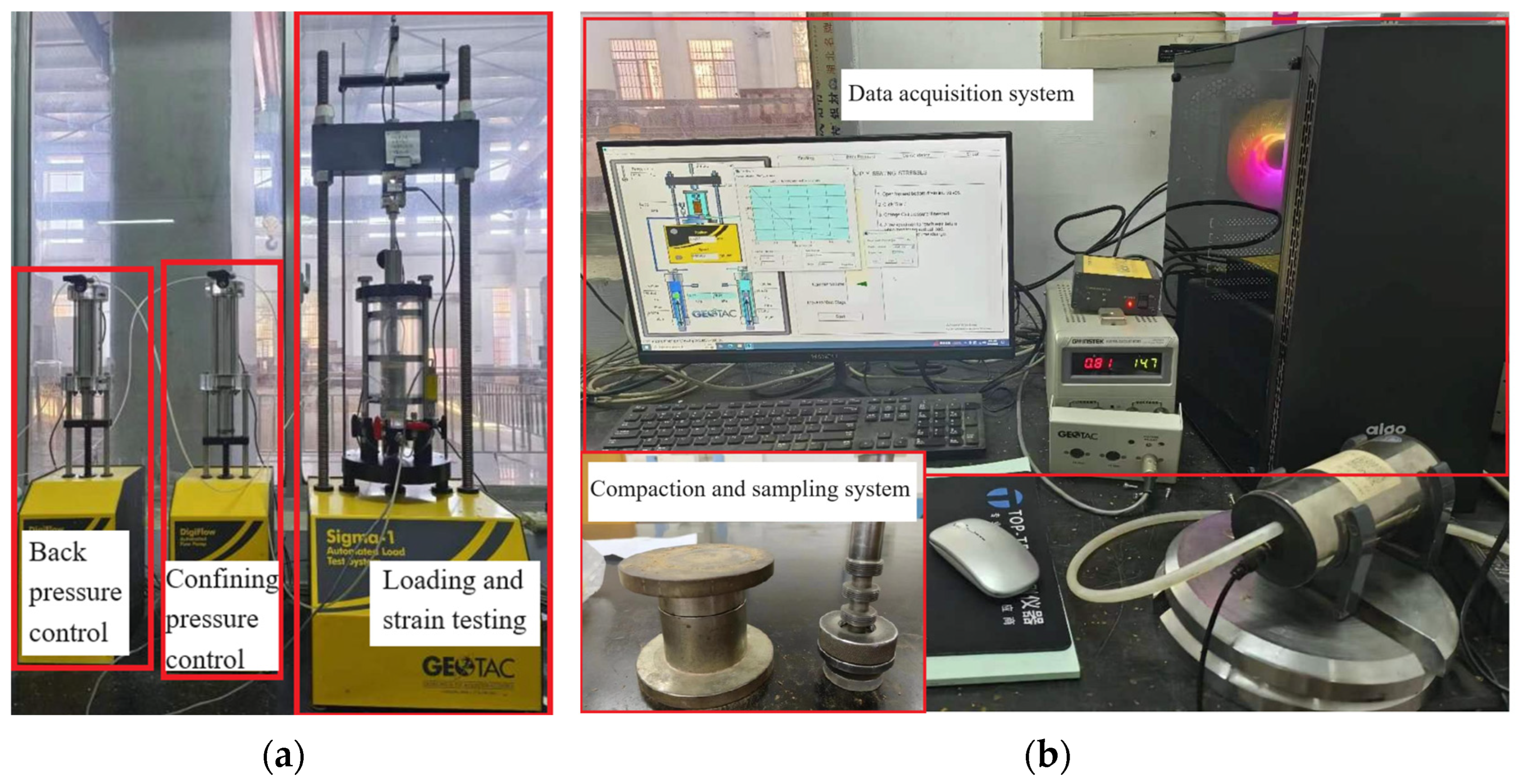
2.2. Static Triaxial Tests under Different Dry Densities

2.2.1. Setting of Compaction Degree

According to the technical specifications for construction of airfield earthwork and pavement base [28], the elevation of the airport site is 1028.60 m, which belongs to excavation or zero fill area, and the compaction degree is greater than 94% within a range of 1 m below the surface. During subsoil compaction, the soil surface is severely compressed under the impact of gravity, and the compaction degree of soil gradually decreases with the increase in depth. Considering the requirements at different depths, soil compaction degrees of 97%, 94%, and 91% were selected to represent the compaction conditions of 0–1 m, 1–4 m, and 4–10 m below the surface, respectively.

2.2.2. Sample Preparation

The preparation of static triaxial sample includes the compaction and saturation process. The diameter and the height of the sample are 39.1 mm and 80 mm, respectively. The dry soil was passed through a sieve with the diameter of 2 mm, then the optimal water content of silt was achieved by mixing with planned water. The silt was placed in a closed container for 24 h. The mass of the layered compaction silt was calculated based on the required dry density. After each layer of the silt sample is compacted, the roughness of the silt surface was increased by scraping treatment. After silt sample preparation, the silt sample was placed into a saturator for air saturation. A confining pressure of 20 kPa was preloaded during the test. The degree of saturation of the silt sample was tested, and if it was below 95%, back pressure saturation was performed until it meets the requirements.

2.2.3. Scheme of Static Triaxial Tests

After the silt sample was saturated, the consolidation undrained test (CU) was carried out according to the standard for the geotechnical testing method [27], where the shear strain rate was taken as 0.2%/min. The test was terminated when the axial strain of samples reached 20%. The tests were performed on soil with the overall compaction degrees of 97%, 94%, and 91%.

The value of confining pressure in static triaxial tests did not influence the shear strength parameters obtained from tests, so the commonly used confining pressures of 100 kPa, 200 kPa, and 300 kPa in static triaxial tests [29] were selected in each test condition. The static triaxial test systems are composed of test instruments, data acquisition system and sample preparation system, which are shown in Figure 1.

2.2.4. Stress–Strain Relationship

The failure mode of silt sample after static triaxial test is shown in Figure 2. It can be seen that no continuous shear failure surface is formed during the triaxial shear process of silt sample with different compaction degrees. The silt mainly undergoes volume expansion. The middle part of the silt sample bulges outward, and it shows a clear failure mode of shear expansion.

Figure 3 shows the stress–strain relationships of soil samples under different compaction degrees (K). The dry density is represented by ρ. As is shown in Figure 3, under different experimental conditions, when axial strain (ε₁) is small, the deviatoric stress (σ₁–σ₃) increases rapidly, and with the increase in strain, the increase rate of deviator stress (σ₁–σ₃) gradually decreases and eventually becomes stable. No peak value occurs during the increase of deviatoric stress, and all soil samples present strain-hardening behavior. Under the same compaction degree, the deformation resistance of the sample increased with the increase in confining pressure, whereas under different confining pressures, the soil generally presents the same deformation trend. Compaction degree has an evident influence on soil strength, and under the same confining pressure, compactness of soil increases, the interaction between particles increases, and the axial loading capacity of the sample increases accordingly.

2.2.5. Effective Stress Path

According to the standard for geotechnical testing method [27], the peak value of deviatoric stress (σ₁–σ₃) is usually taken as the failure point. When the deviatoric stress has no obvious peak value, the dense point of the effective stress path or the stress point corresponding to a certain axial strain (generally taken as ε₁ = 15%) should be selected as the failure point. The parameters of the failure point are selected based on the denseness of stress state points near the terminal point of the effective stress path.

Table 1. Failure points of the samples under different compaction degrees.

Compaction Degree (%)	Density/g·cm−3	Confining Pressure/kPa	Deviatoric Stress p/kPa	Deviatoric Stress q/kPa	Gradient of Failure Line M/Dimensionless
91%	1.729	100	365.615	516.226	1.401
		200	375.919	525.465
		300	450.832	629.578
94%	1.786	100	648.019	921.356	1.436
		200	660.629	940.698
		300	680.982	966.539
97%	1.843	100	640.030	929.639	1.443
		200	786.851	1136.976
		300	793.653	1138.780

enlists the failure points of the samples under different compaction degrees.

In static triaxial test, p and q are the deviatoric stress. p = (σ₁ + σ₂ + σ₃)/3, σ₂ = σ₃, q = σ₁–σ₃, and q = Mp. σ₁, σ₂, and σ₃ can be tested by static triaxial test. As seen in Table 1, the compaction degree has minimal influence on the soil damage line, and it can be considered that the compaction degree does not influence the gradient of the soil damage line (M). The value of M is unified taken as 1.4.

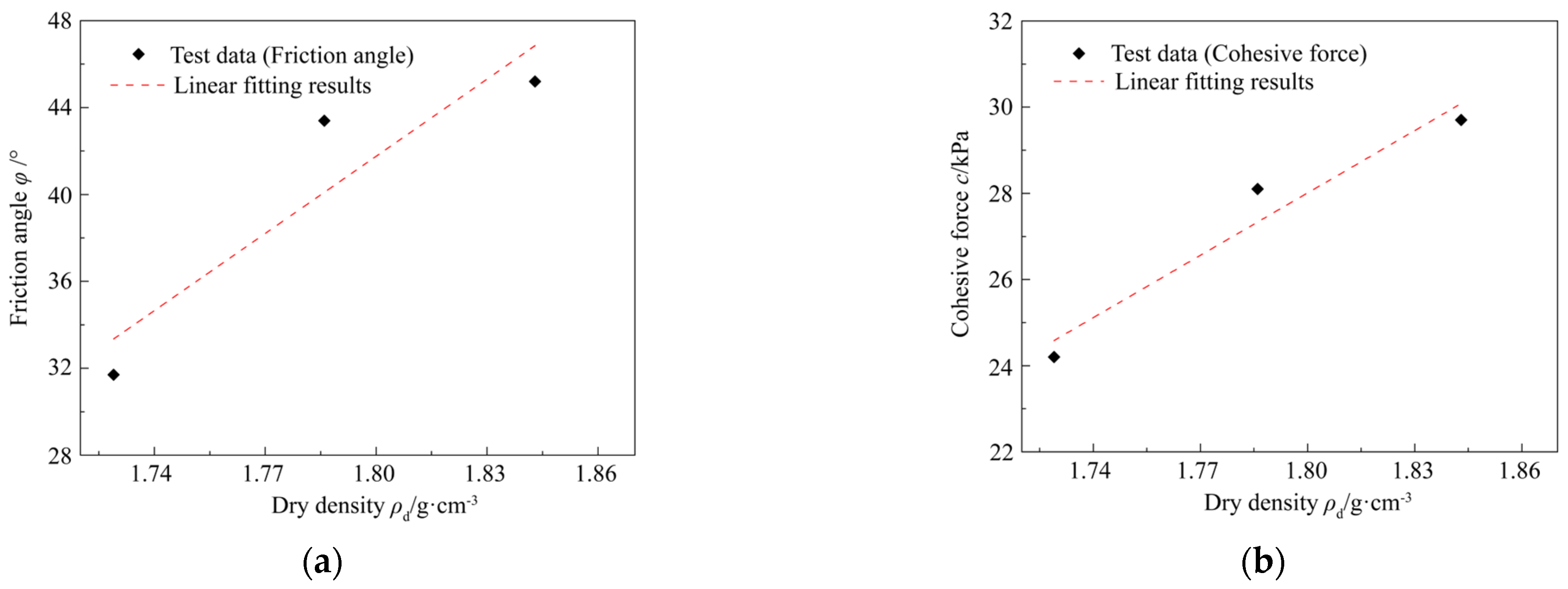
2.2.6. Analysis of Shear Strength Parameters

In the study, the Mohr–Coulomb strength theory is used to investigate the differences in the shear strength of soil caused by different compaction degrees.

$$S=c+\sigma \tan \varphi$$

(1)

where, S represents shear strength (kPa); c represents cohesion force (kPa), σ represents the normal stress (kPa), and φ represents the internal friction angle (°).

Figure 4 shows the correlation relationship between the shear strength parameters and dry density. The dry density of the samples significantly affects the shear strength parameters of the soil. The strength index of the soil increases with the increase of dry density, and the strength index of the soil exhibits a linear relationship with the dry density of the samples. The reason is that the increase in dry density of the samples leads to the decreased soil porosity, the increased contact area of particles, the increased bonding, and the increased cohesive force. It also leads to the enhanced interaction between soil particles, the enhanced deformation resistance ability, and the increased internal friction angle.

Friction angle, cohesion force, and dry density present a linear relationship, and the expression of their fitting relationship are as follows:

$$\varphi =-171.4000+118.4210{\rho }_d,R^2=0.8897$$

(2)

$$c=-58.8333+48.2456{\rho }_d,R^2=0.9056$$

(3)

3. Boundary Surface Model and Numerical Implementation

3.1. Boundary Surface Model

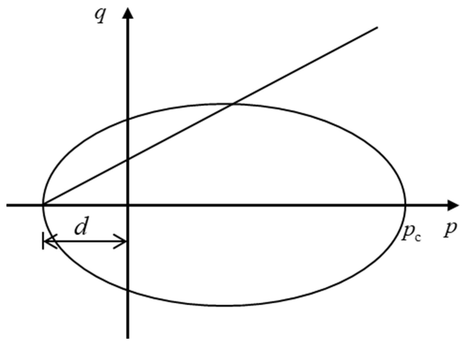
3.1.1. Boundary Surface Equation

In the manuscript, the Z-P criterion yield curve proposed by Zienkiewicz–Pande [30] was adopted. The yield curve is smooth on the p-q meridian plane and π plane. The relationship between the yield curve and hydrostatic pressure, as well as the influence of the intermediate principal stress (σ₂) on the yield curve was considered, which facilitated numerical calculations. The equation is given as Equation (4).

$${\left[\frac{\overline{p}-\frac{1}{2}(p_c-d)}{\frac{1}{2}\left(p_c+d\right)}\right]}^2+{\left[\frac{\overline{q}}{\frac{1}{2}M\left({\theta }_{\sigma }\right)(p_c+d)}\right]}^2=1$$

(4)

where, $p=\frac{{\sigma }_1+2{\sigma }_3}{3}$; $q={\sigma }_1-{\sigma }_3$; σ₁ and σ₃ are the effective stress in the respective direction; $\overline{p}$ represents virtual average stress; $\overline{q}$ represents virtual deviatoric stress; $M\left({\theta }_{\sigma }\right)$ is the curve shape function of the boundary surface in π plane; ${\theta }_{\sigma }$ is the Lode angle. $d=c\cot \varphi$; c is the cohesive force, and φ is the internal friction angle. $p_c$ is the pre-consolidation pressure. Figure 3 shows the shape of the boundary surface in p-q plane. The shape of the boundary surface is shown in Figure 5.

According to Equations (2) and (3), d can be expressed by Equation (5).

$$d=\left(-58.8333+48.2456{\rho }_d\right)\cot \left(-171.4000+118.4210{\rho }_d\right)$$

(5)

3.1.2. Reflection Principles

In the study, the interpolation function proposed by Huang and Song [17], and Huang et al. [22] was used as the interpolation function of plastic modulus. The equation is given as follows:

$$K_p=\overline{K_p}+P_a\xi \left[{\left(\frac{\partial F}{\partial \overline{p}}\right)}^2+{\left(\frac{\partial F}{\partial \overline{q}}\right)}^2\right]\left[{\left(\frac{{\delta }_0}{{\delta }_0-\delta }\right)}^u-1\right]$$

(6)

$$u=u_0\exp \left(-\varsigma {\epsilon }_s^p\right)$$

(7)

where, K_p is the actual plastic modulus. $\overline{K_p}$ is the plastic modulus of mapping points on the boundary surface. P_a represents atmospheric pressure. The parameter u denotes the influence of strain history on plastic modulus. u₀ and $\varsigma$ are model parameters. ${\epsilon }_s^p$ is the cumulative plastic shear strain in the cycle process. ${\delta }_0$ is the distance from the virtual stress point to the mapping center. $\delta$ is the distance from the true stress point to the virtual stress point.

3.1.3. Flow Rule

According to the associated flow rule, the plastic flow direction is considered equal to the plastic loading direction. So, the plastic volume strain $d{\epsilon }_v^p$ and the plastic shear strain $d{\epsilon }_s^p$ are presented in Equation (8).

$$d{\epsilon }_v^p=L\frac{\partial F}{\partial p},d{\epsilon }_s^p=L\frac{\partial F}{\partial q}$$

(8)

where, ${\epsilon }_v^p$ is the plastic volume strain. ${\epsilon }_s^p$ is the plastic shear strain, and L is the plastic scalar factor.

3.1.4. Hardening Rule

The isotropic hardening rule was used. The size of yield surface was changed rather than the shape, and the change in size of yield surface was only related to the plastic volume strain ${\epsilon }_v^p$. The equation is given as follows:

$$d{p}_c=p_c\frac{1+e_0}{\lambda -k}d{\epsilon }_v^p$$

(9)

where, P_c is the pre-consolidation pressure; e₀ is the initial void ratio; λ and κ are the gradients of the normal compression and rebound curves of e-lnp.

3.1.5. Plastic Modulus

By applying the consistency condition ($dF=0$) to Equations (8) and (9), Equation (10) can be obtained.

$$\overline{K_p}=-\frac{\partial F}{\partial p_c}\frac{\partial p_c}{\partial {\epsilon }_v^p}\frac{\partial G}{\partial \overline{p}}$$

(10)

According to the equation of the yield surface and the associated flow rule, the following equation can be obtained as follows:

$$\overline{K_p}=\left(\overline{p}+d\right)p_c\overline{p}\frac{1+e_0}{\lambda -k}\left(2\overline{p}-p_c+d\right)$$

(11)

3.1.6. Loading Criteria

The following modes were taken for the loading criteria in the study.

$\frac{\partial F}{\partial {\sigma }_{ij}}d{\epsilon }_{ij}>0$, the loading state.

$\frac{\partial F}{\partial {\sigma }_{ij}}d{\epsilon }_{ij}=0$, the neutral state.

$\frac{\partial F}{\partial {\sigma }_{ij}}d{\epsilon }_{ij}<0$, the unloading state.

3.2. Numerical Implementation

In the study, the improved Euler integral algorithm [30] was used. The strain increment ($\Delta {\epsilon }_{n+1}$) was divided into a series of substrain increments according to time so that the substrain increment ($\Delta {\epsilon }_{ss}$) can be given as $\Delta {\epsilon }_{ss}=\Delta T\Delta {\epsilon }_{n+1}$. The time increment of the substep length ($\Delta T, 0<\Delta T<1$) was controlled by astringency and error criteria. The UMAT subprogram was programmed in ABAQUS by Fortran language to realize the boundary surface model of remolded saturated silt mentioned above.

By comparing the dynamic triaxial test results of silt with different compaction degrees in the literature [31], the consolidated undrained dynamic triaxial test was conducted for simulation and verification. In the dynamic triaxial test, the diameter and the height of the cylindrical samples are 39.1 mm and 80 mm, respectively. At the beginning of the test, isotropic stress was applied to the samples, and isotropic consolidation was carried out. After the samples were consolidated and stabilized, vertical load (σ_d) was applied. A half-sine waveform with a frequency of 1 Hz was used for the dynamic load.

Table 2. Dynamic triaxial simulation scheme.

Samples	Dynamic Stress Ratio	Frequency/Hz	Dry Density/g·cm−3	Void Ratio
A	0.30	1	1.80	1.14
B	0.45		1.86	0.97
C	0.50		1.79	1.16

presents the simulation scheme for the dynamic triaxial test, while

Table 3. Material parameters of saturated silt samples with different dry densities.

Samples	Cohesive Force/kPa	Internal Friction Angle/°	Compression Gradient λ	Rebound Gradient κ	Poisson’s Ratio ν	Gradient of Failure Line M	Model Constant $\mathit{\xi }$	Atmospheric Constant /kPa	Model Constant $\mathit{\varsigma }$
A	28.0	41.75	0.25	0.15	0.2	1.4	10	101.325	3.225
B	30.9	48.86
C	27.5	40.57

enlists the material parameters of saturated silt samples with different dry densities. In the study, the number of cyclic vibrations in the test reached 10⁵, and the development trend of the cumulative strain of the samples stabilized after 1000 cycles. In the study, only the first 1000 loading cycles were simulated.

Figure 6 compares the experimental results of the dynamic triaxial test and simulation results with the confining pressure of 80 kPa. The development trend of the simulated cumulative axial strain is consistent with that of the experimental results, with minor deviations, and the maximum error is near 10%. The error of sample B is relatively large because there is a certain deviation in the simulation of small deformation. In the actual dynamic triaxial test, as the cumulative strain reaches 10%, the standard for stopping the test is achieved, and it is easy to achieve better simulation effects in the simulation of large deformation. Therefore, the constitutive model established in the study can better reflect the dynamic characteristics of saturated silt and describe the development trend of cumulative axial strain in saturated silt accurately.

4. Numerical Simulation of Subsoil Deformation

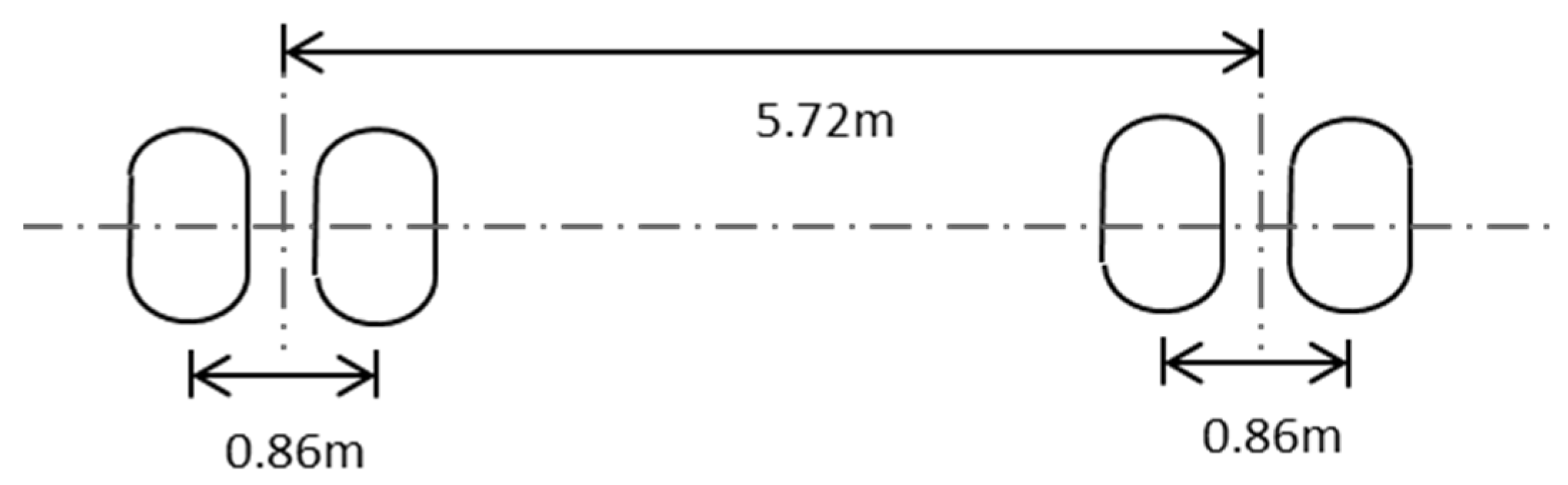
4.1. Simulation of Aircraft Loading

In the study concerning aircraft loading, only the moving load during aircraft sliding was studied. B-737-800, a typical aircraft type, was selected for numerical simulation of silt subsoil deformation under aircraft loading. Moving constant loading and moving vibration loading were used to simulate the aircraft loading. The type of vibration loading was regarded as stable sine waves. Considering aircraft weight and the impact of aircraft lift, the mathematical relationship model of dynamic load coefficient, aircraft sliding speed, and international roughness index (IRI) for airport pavement was used [32]. The maximum dynamic load coefficient of 1.1576 in the most unfavorable condition is taken, i.e., at the speed of 15 m/s, and the diameter of the outer tire is 1.105 m [33].

In the existing pavement design methods, a rectangle and two semicircles are generally used to represent wheel marks. The load was simplified into a rectangle distributed loading through equivalent analysis, which was convenient for grid division and loading arrangement in finite element analysis [34]. The thickness of the tires and the moving direction of the aircraft have no influence on the distribution characteristics of the aircraft loading. Figure 7 shows the wheel marks of the main landing gear for B-737-800.

With the sliding speed of 15 m/s for B-737-800, the relationship between pressure and time was obtained as follows:

$$P_{737}=1212.70+191.12\sin (27.14t)(\mathrm{kPa})$$

(12)

When the aircraft first slid, the maximum and minimum values of the aircraft loading appeared at the time points of 0.3 s and 1.1 s, respectively. In addition, the speeds of 10 m/s and 20 m/s were taken as the control group for follow-up analysis, and the dynamic load coefficients under the speed of 10 m/s and 20 m/s were taken as 1.1470.

The editable UMAT subroutine provided by numerical analysis software (ABAQUS 6.14) was applied to write the code of the moving load at a certain speed in the load-moving zone, and then the written subroutine was applied in numerical analysis software (ABAQUS 6.14). The numerical calculation model is established in finite element numerical analysis software (ABAQUS 6.14). The subprogram was written in Fortran language.

4.2. Simulation Scheme

According to the literature [35], the pavement surface, base layer, and cushion layer of the airport runway were all simulated by the elastic model.

Table 4. Material parameters of each pavement layer.

Layers	Material Types	Thickness /cm	Density /kg·m−3	Elastic Modulus /MPa	Poisson’s Ratio	Damping
Pavement surface	Cement concrete	36	2400	32,900	0.167	0.8
Base layer	Cement stabilized macadam	30	2300	3000	0.30	0.8
Cushion layer	Natural grit	30	2300	1200	0.35	0.8

presents the material parameters of each runway layer. The materials of the silt subsoil were given to different runway layers according to different compaction degrees. In combination with the above-mentioned triaxial test results, material parameters of the silt at different depth of the subsoil are shown in

Table 5. Material parameters of the silt at different depth of the subsoil.

Depth/m	Cohesive Force/kPa	Internal Friction Angle/°	Compression Gradient λ	Rebound Gradient κ	Poisson’s Ratio ν	Gradient of Failure Line M	Model Constant $\mathit{\xi }$	Atmospheric Constant /kPa	Model Constant $\mathit{\varsigma }$
0–1	29.7	45.2	0.016	0.005	0.3	1.4	10	101.325	1.225
1–4	28.1	43.4
4–10	24.2	38.4

. The total thickness of the airport runway is 10.96 m.

In the numerical model established by the finite element analysis software (ABAQUS 6.14), X represents the transverse direction of the airport runway. Y was the heading direction of the aircraft, and Z was the depth direction of the runway. The deformation at the bottom of the model was restricted, and the transverse deformation at the side of the model was restricted. Figure 8 shows the grid division of the runway model. ‘C3D8P’ represents the pore pressure element, and ‘C3D8R’ represents the plane stress element in software (ABAQUS 6.14). ‘C3D8R’ unit was used as the grid type of the pavement surface, base layer, and cushion layer. Considering the effect of pores and seepage, ‘C3D8P’ unit was used as the grid type of the silt subsoil, and grid refinement was performed only on the main scope affected by aircraft loading in grid division.

A case study was conducted on B-737-800 aircraft to investigate the subsoil deformation under cyclic loading. In total, 50 cycles were studied initially to evaluate the preliminary development trend of cyclic loading. The aircraft speed was 15 m/s, and the length, width, and height of the numerical model were 30 m, 20 m, and 10.96 m, respectively. The compaction degrees of the subsoil in the ranges of 0–1 m, 1–4 m, and 4–10 m were 97%, 94%, and 91%, respectively, and the subsoil model with the overall compaction degree of 94% was set as the control group.

4.3. Analysis of Subsoil Deformation Results

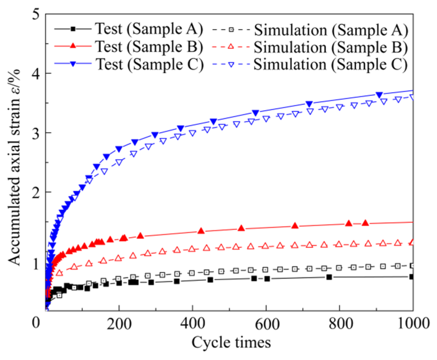
4.3.1. Impact Analysis of Cyclic Loading

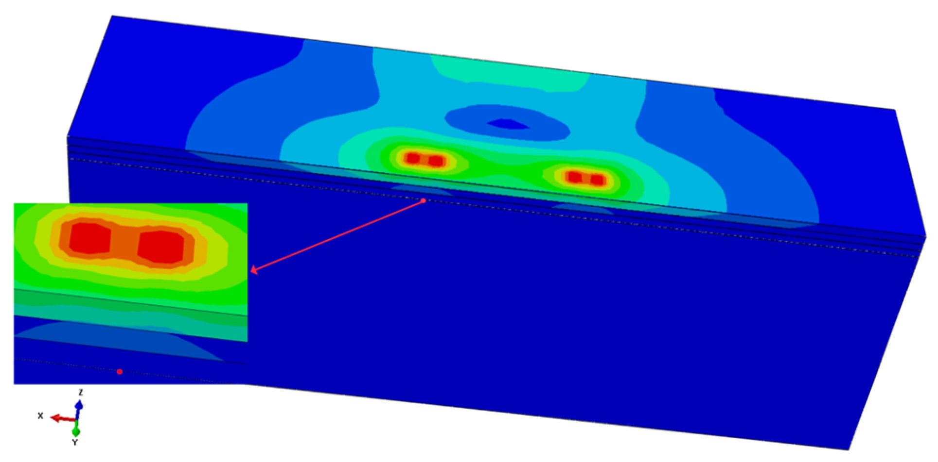
Deformation Analysis of Single Point

Analysis of subsoil deformation under cyclic loading was carried out with the aircraft type of B-737-800. Figure 9 shows the reference points under the cyclic loading during the process of aircraft sliding.

Figure 10 shows the vertical deformation diagram of the reference point under the moving cyclic loading. When the aircraft loading was loaded for the first time, the elastic deformation of 5 mm was quickly generated on the surface of the silt subsoil. As the aircraft passed, the elastic deformation recovered, and the plastic deformation accumulated at this point. The development trend of the elastic deformation was different from the stable development state of deformation in results of dynamic triaxial tests, because the model is larger, and the time increment step is too large to converge during the calculation process of ABAQUS. ABAQUS automatically reduces the step size and continues the analysis, which results in slight differences in results of elastic deformation.

In dynamic triaxial tests, the limit standard for the plastic stable state of soil fillers is obtained when the development rate of the plastic strain reaching 10⁻⁵ [36,37]. As is shown in Figure 10, as the number of loading cycles increases, the volume of silt porosity decreases rapidly. The deformation of silt caused by the decrease of porosity volume gradually decreases, so the rate of development of deformation decreases. when the number of cycles is 50, the vertical deformation on the surface of the silt subsoil reaches 3.65 mm. The cumulative plastic deformation is from 3.43 mm to 3.65 mm, as the cyclic times varies from 30 to 50. According to the relationship between small strain and deformation, as the depth of the silt subsoil is 10 m, the surface strain of silt subsoil is about 8 × 10⁻⁶ when the cyclic times varies from 30 to 50. After 50 cycles of dynamic loading, the porosity volume of the silt is very small, and the compressibility of the silt is low. Therefore, when the number of cycles reaches 50, it is considered that the silt subsoil initially reached a stable state.

By comparing the deformation of the subsoil with layered compaction and that with the overall compaction degree of 94% under moving cyclic loading, the deformation of single point on subsoil with different compaction conditions under cyclic loading is shown in Figure 11.

Table 6. Vertical deformation on the surface of the silt subsoil.

Compaction Degree	Maximum Vertical Deformation/mm (t = 0.3 s)	Maximum Vertical Deformation/mm (t = 1.1 s)
94%	2.15	1.50
97%, 94%, 91%	2.20	1.52

shows the vertical deformation on the surface of the silt subsoil with different compaction conditions at different time during the single sliding of aircraft.

Seen from Figure 11, the two conditions present the same deformation development trend as the number of cycle increases. However, due to the lower compaction degree (91%) of soil at the bottom of the subsoil with layered compaction, the load transferred to the bottom of the subsoil leads to greater deformation. Therefore, in the analysis process of cyclic loading, the vertical deformation generated by layered compaction is greater than that of the subsoil with an overall compaction degree of 94%. The ratio of the cumulative plastic deformation of the subsoil under layered and overall compaction after each loading cycle is shown in Figure 11. The ratio is larger in the initial loading process, because the initial plastic deformation of the subsoil with the overall compaction degree of 94% is minimal. As the number of cycles increase, the ratio of the cumulative plastic deformation decreases first and then stays stable. The maximum deformation under two conditions in the initial loading process are similar. However, with the increase of loading cycles, the cumulative plastic deformation of the subsoil with the overall compaction degree of 94% reaches about 1.25 mm, and the ratio of the cumulative plastic deformation of the subsoil finally reaches 2. It indicates that the long-term deformation of silt subsoil under actual compaction conditions may exceed the limit. Therefore, in actual engineering, the compaction degree of the subsoil with the depth from 4 m to 10 m should be attached more importance, when the subsoil is compacted by layers.

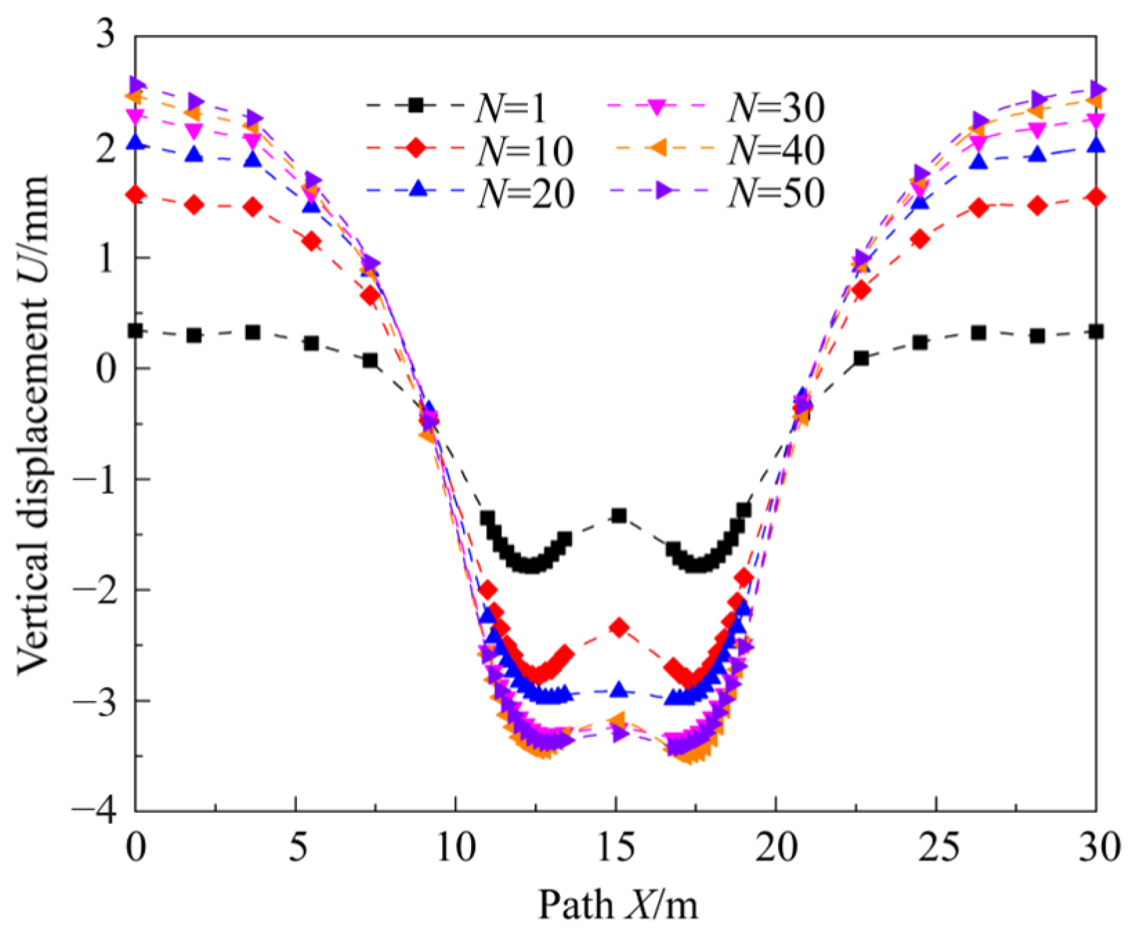
Analysis of Overall Deformation

On the top of the silt subsoil (Z = 10 m), the path in the middle of the subsoil (Y = 10 m) was selected to analyze the overall deformation of the silt subsoil under cyclic loading. Figure 12 shows the vertical deformation of the runway under different loading cycles. The vertical deformation under the concentration area of aircraft loading gradually increased with the increase of cycles. The maximum instantaneous deformation at the top of the silt subsoil under initial loading was about 2 mm. When the number of cycles increased from 1 to 10, the increase extent of vertical deformation is about 77.07%. As the number of cycles increased to 50, the increase of deformation decreased gradually. The vertical deformation stayed stable with 30 to 50 cycles, and the increase extent of vertical deformation is about 1.66%. When the concrete panel was regarded as a whole, the subsoil was subjected to instantaneous loading locally, which caused the subsoil hollow under the action area of aircraft loading. It also led to the slight upwarp of the surrounding pavement slabs. As the loading cycle increases from 1 to 10, the upward deformation on the edge of pavement slabs increased significantly. As the loading cycles increase, the increase of vertical deformation gradually decreased and then stayed stable.

4.3.2. Impact Analysis of Load Frequency

When B-737-800 aircraft moved at the speed of 10 m/s and 20 m/s, the relationship between airport loading and time were given as follows:

$$P_{10}=1212.70+178.26\sin (18.10t)(\mathrm{kPa})$$

(13)

$$P_{20}=1212.70+178.26\sin (36.20t)(\mathrm{kPa})$$

(14)

The cumulative deformation of the silt subsoil was analyzed when the aircraft moved at the speed of 10 m/s and 20 m/s, respectively. The influence of loading frequency on the deformation of layered compaction subsoil was studied. Figure 13 showed the development trend of vertical deformation on the surface of the subsoil under different loading cycles. When the moving speed of the aircraft changed, the simulation result of subsoil deformation changed. The development trend of deformation stayed unchanged under different moving speed of aircraft. Obvious phenomena of elastic deformation and plastic residual deformation were observed. At the initial loading stage, when aircraft moved at a speed of 20 m/s, the plastic deformation on the surface of the silt subsoil increased rapidly. The plastic deformation gradually stabilized as load cycles increased, and the increase rate decreased. The strain developed rapidly when the aircraft moved at the speed of 10 m/s. The reason was that the plastic deformation could not be formed completely when the speed increased. When the aircraft moved at the speed of 10 m/s, with the sufficient retention time of aircraft loading, the plastic deformation developed adequately.

Compared with Figure 10, the main influencing factor of the subsoil deformation was the value of aircraft loading under different loading frequencies. Therefore, appropriate parameters of compaction degree in layered compacted subsoil are important to control the subsoil deformation under the maximum aircraft loading, so as to meet the requirements of the specification.

5. Conclusions

Based on the dynamic and static parameters of remolded silt, a dynamic constitutive model for remolded saturated silt that could consider the effect of dry density was established. The UMAT material subprogram was developed and written. The validity and accuracy of the numerical model developed in the study were verified by the simulation results of dynamic triaxial tests. The main conclusions are as follows:

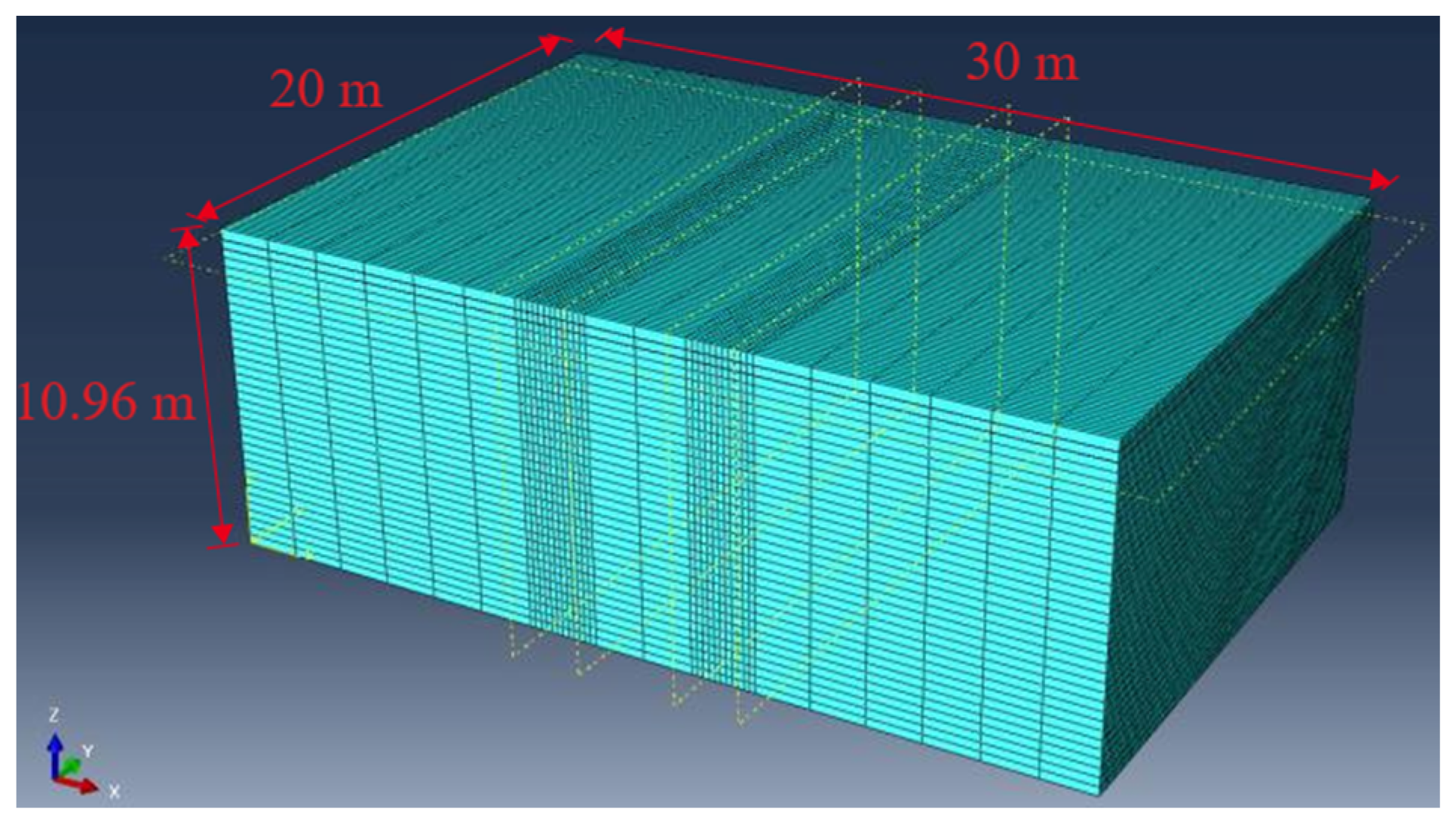
• Based on the layered filling of the silt subsoil of Hohhot new airport, the numerical model of airport runway is established. Based on the established dynamic constitutive model for remolded saturated silt, through the UMAT subprogram, the moving cyclic loading of aircraft on the pavement was achieved. Through numerical simulation, the influence of compaction degree on the deformation of silt subsoil under moving cyclic loading of aircraft was revealed.
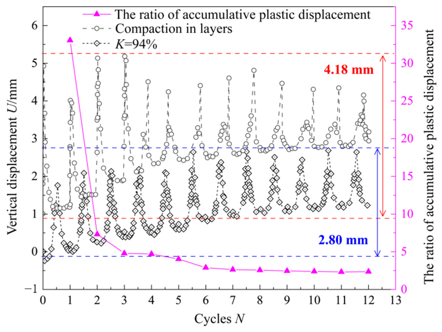
• As the number of cycles increase, the development rate of deformation gradually decreases, and the deformation of silt subsoil stays stable after 50 loading cycles. The cumulative plastic deformation of the saturated subsoil compacted by layers under 50 cycles of dynamic aircraft loading reaches 3.65 mm. After the same loading cycles, the cumulative plastic deformation of the subsoil with layered compaction is twice than that with overall compaction. This indicates that the selection of combined parameters of compaction degree is crucial for the subsoil compacted in layers.
• A control group with different speeds of 10 m/s and 20 m/s was set to explore the influence of loading frequency on subsoil deformation. The development trends of cumulative plastic deformation stays unchanged as the aircraft speed is 15 m/s. At the aircraft speed of 10 m/s, the long residence time of loading makes it easier to form accumulative plastic deformation. Therefore, in practical engineering, to ensure that the compaction degree of subsoil meets the requirements of long-term deformation control, the compaction degrees of subsoil with the depth from 4 m to 10 m should be controlled and paid more importance.

References

1. Chen, Q.; Indraratna, B. Deformation behavior of lignosulfonate-treated sandy silt under cyclic loading. J. Geotech. Geoenvironmental Eng. 2015, 141, 06014015.1–06014015.5. [Google Scholar] [CrossRef]
2. Chen, Q.; Indraratna, B. Shear behaviour of sandy silt treated with lignosulfonate. Can. Geotech. J. 2015, 52, 1180–1185. [Google Scholar] [CrossRef]
3. Subei, N.; Saxena, S.K.; Mohammadi, J. A BEM–FEM approach for analysis of distresses in pavements. Int. J. Numer. Anal. Methods Geomech. 2010, 15, 103–119. [Google Scholar] [CrossRef]
4. Luo, Q.; Ye, X.; Li, Q.; Zhang, S.; Yu, Q.; Ma, X. Experimental and numerical study on response characteristics of airport pavement subjected to wetting in silt subgrade. KSCE J. Civ. Eng. 2023, 27, 551–566. [Google Scholar] [CrossRef]
5. Monismith, C.L.; Ogawa, N.; Freeme, C.R. Permanent deformation characteristics of subsoil soils due to repeated loading. Transp. Res. Rec. J. Transp. Res. Board 1975, 537, 1–17. [Google Scholar]
6. Li, J. Permanent Deformation and Resilient Modulus of Unbound Granular Materials; Iowa State University: Ames, IA, USA, 2013. [Google Scholar]
7. Anand, J.P.; Louay, N.M.; Aaron, A. Permanent deformation characterization of subgrade soils from RLT test. J. Mater. Civ. Eng. 1999, 11, 274–282. [Google Scholar]
8. Salour, F.; Erlingsson, S. Permanent deformation characteristics of silty sand subgrades from multistage RLT tests. Int. J. Pavement Eng. 2017, 18, 236–246. [Google Scholar] [CrossRef]
9. Tang, L.; Yan, M.H.; Ling, X.Z.; Tian, S. Dynamic behavioursof railway’s base course materials subjected to long-term low-level cyclic loading: Experimental study and empirical model. Géotechnique 2016, 67, 537–545. [Google Scholar] [CrossRef]
10. Ren, X.W.; Xu, Q.; Teng, J.D.; Zhao, N.; Lv, L. A novel model for the cumulative plastic strain of soft marine clay under long-term low cyclic loads. Ocean. Eng. 2018, 149, 194–204. [Google Scholar] [CrossRef]
11. Mróz, Z. On the description of anisotropic workhardening. J. Mech. Phys. Solids 1967, 15, 163–175. [Google Scholar] [CrossRef]
12. Koiter, W.T. Stress-strain relations, uniqueness and variational theorems for elastic- plastic materials with a singular yield surface. Q. Appl. Math. 1953, 11, 350–354. [Google Scholar] [CrossRef]
13. Iwan, W.D. On a class of models for the yielding behavior of continuous and composite systems. J. Appl. Mech. 1967, 34, 612–617. [Google Scholar] [CrossRef]
14. Prevost, J.H. Anisotropic undrained stress-strain behavior of clays. J. Geotech. Eng. Div. ASCE 1978, 104, 1075–1090. [Google Scholar] [CrossRef]
15. Mrǒz, Z.; Norris, V.A.; Zienkiewicz, O.C. An anisotropic hardening model for soils and its application to cyclic loading. Int. J. Numer. Anal. Methods Geomech. 1978, 2, 203–221. [Google Scholar] [CrossRef]
16. Wan, Z.; Gao, W.S.; Xie, L.Y. Elastoplastic Model for Sand and Clay Suitable for Describing the Cyclic Loading Response. Strength Mater. 2021, 53, 662–669. [Google Scholar] [CrossRef]
17. Huang, M.S.; Song, C.X. Upper-bound stability analysis of a plane strain heading in non-homogeneous clay. Tunneling Undergr. Space Technol. 2013, 38, 213–223. [Google Scholar] [CrossRef]
18. Mróz, Z.; Norris, V.A.; Zienkiewicz, O.C. Application of an anisotropic hardening model in the analysis of elastoplastic deformation of soils. Geotechnique 1979, 299, 1–34. [Google Scholar] [CrossRef]
19. Srinil, C.; Komolvilas, V.; Kikumoto, M. Unified state boundary surface model for clay and sand under saturated and unsaturated conditions. Soils Found. 2022, 62, 101219. [Google Scholar] [CrossRef]
20. Jockovic, S.; Vukicevic, M. Bounding surface model for over-consolidated clays with new state parameter formulation of hardening rule. Comput. Geotech. 2017, 83, 16–29. [Google Scholar] [CrossRef]
21. Masin, D. Clay hypoplasticity model including stiffness anisotropy. Géotechnique 2015, 64, 232–238. [Google Scholar] [CrossRef]
22. Huang, M.S.; Liu, Y.H.; Sheng, D.C. Simulation of yielding and stress-stain behavior of shanghai soft clay. Comput. Geotech. 2011, 38, 341–353. [Google Scholar] [CrossRef]
23. Cun, H.; Liu, H. A new bounding-surface plasticity model for cyclic behaviors of saturated clay. Commun. Nonlinear Sci. Numer. Simul. 2015, 22, 101–119. [Google Scholar]
24. Manzari, M.T.; Yonten, K. On implementation and performance of an anisotropic constitutive model for clays. Int. J. Comput. Methods 2014, 11, 1342009. [Google Scholar] [CrossRef]
25. Heidarzadeh, H.; Kamgar, R. Necessity of applying the concept of the steady state on the numerical analyses of excavation issues: Laboratory, field and numerical investigations. Geomech. Geoengin. 2020, 17, 413–425. [Google Scholar] [CrossRef]
26. Qin, L. Dynamic Constitutive Model of Unsaturated Loess and Its Application in Seismic Response Analysis of Subway Station. Ph.D. Thesis, Chang’an University, Chang’an, China, 2010. (In Chinese). [Google Scholar]
27. GB/T 50123—2019; Ministry of Housing and Urban-Rural Development of the People’s Republic of China. Standard for Geotechnical Testing Method. China Planning Press: Beijing, China, 2019. (In Chinese)
28. MH/T 5014—2022; Civil Aviation Administration of China. Technical Specifications for Construction of Airfield Earthwork and Pavement Base. China Civil Aviation Publishing House: Beijing, China, 2022. (In Chinese)
29. Ma, X.; Yu, Q.; Xuan, M.; Ren, H.; Ye, X.; Liu, B. Study on the influence mechanism of sample preparation method on the shear strength of silty soil. Sustainability 2023, 15, 2635. [Google Scholar] [CrossRef]
30. Zienkiewicz, O.C. The Finite Element Method in Engineering Science; McGraw-Hill: London, UK, 1971. [Google Scholar]
31. Huang, B.; Ding, H.; Chen, Y. Simulation of high-speed train load by dynamic tests. Chin. J. Geotech. Eng. 2011, 55, 195–201. (In Chinese) [Google Scholar]
32. Fu, Y.-K.; Li, Y.-L.; Tan, Y.-Q.; Zhang, C. Dynamic response analyses of snow-melting airport rigid pavement under different types of moving loads. Road Mater. Pavement Des. 2019, 20, 943–963. [Google Scholar] [CrossRef]
33. Qin, L. Study on Deformation of Airport Pavement Foundation under the Action of Aircraft Loads and Groundwater. Master’s Thesis, Zhengzhou University, Zhengzhou, China, 2017. (In Chinese). [Google Scholar]
34. Guo, H.; Sherwood, J.A.; Snyder, M.B. Component Dowel-Bar Model for Load-Transfer Systems in PCC Pavements. J. Transp. Eng. ASCE 1995, 121, 289–298. [Google Scholar] [CrossRef]
35. Gu, W.J.; Tian, Y.; Zhang, X.Y. Mechanical response and structure optimization of nanomodified asphalt pavement. Adv. Civ. Eng. 2021, 2021, 6286704. [Google Scholar] [CrossRef]
36. Li, Y.B.; Zhang, J.S.; Zhu, Z.H.; Wang, X.; Shi, X. Study on dynamic characteristics of coarse grained soil filler in railway subsoil under stepped axial cyclic loading. J. Railw. Sci. Eng. 2019, 16, 620–628. [Google Scholar]
37. Gidel, G.; Breysse, D.; Hornych, P.; Chauvin, J.J.; Denis, A. A new approach for investigating the permanent deformation behavior of unbound granular material using the repeated load triaxial apparatus. Bull. De Liaison Des Lab. Des Ponts Et Chaussees 2001, 233, 5–21. [Google Scholar]
Figure 1. The static triaxial test system. (a) Test instruments; (b) Data acquisition and sample preparation system.
Electronics 13 00520 g001
Figure 2. The failure mode of static triaxial sample.
Electronics 13 00520 g002
Figure 3. Stress–strain relationship of soil under different compaction degrees. (a) ρ = 1.729 g/cm3, K = 91%; (b) ρ = 1.786 g/cm3, K = 94%; (c) ρ = 1.843 g/cm3, K = 97%.
Electronics 13 00520 g003
Figure 4. Correlation between shear strength parameters and dry density. (a) The fitting relationship of the internal friction angle and dry density; (b) The fitting relationship of the cohesive force and dry density.
Electronics 13 00520 g004
Figure 5. Shape of the boundary surface.
Electronics 13 00520 g005
Figure 6. Comparison between the experimental results of dynamic triaxial test and simulation results with the confining pressure of 80 kPa.
Electronics 13 00520 g006
Figure 7. Wheel marks of the main landing gear for B-737-800.
Electronics 13 00520 g007
Figure 8. The grid meshing of airport runway.
Electronics 13 00520 g008
Figure 9. Reference points under cyclic loading during the process of aircraft sliding.
Electronics 13 00520 g009
Figure 10. Vertical deformation of the reference point under the moving cyclic loading.
Electronics 13 00520 g010
Figure 11. Deformation at a single point of the subsoil with different compaction conditions.
Electronics 13 00520 g011
Figure 12. Vertical deformation on the surface of aircraft runway with different loading cycles.
Electronics 13 00520 g012
Figure 13. The vertical deformation on the surface of the subsoil with different moving speed of aircraft.
Electronics 13 00520 g013