Multi-Objective Prediction of the Sound Insulation Performance of a Vehicle Body System Using Multiple Kernel Learning–Support Vector Regression

Abstract

The sound insulation performance of an electric vehicle’s body system serves as a critical metric for evaluating the noise, vibration, and harshness (NVH) quality of the vehicle. The accurate and efficient prediction of sound insulation performance is foundational for undertaking noise reduction design and optimization. Current engineering practices predominantly rely on Computer-Aided Engineering (CAE) methodologies to address this challenge. However, inherent shortcomings such as low modeling efficiency and difficulty in ensuring prediction accuracy often characterize these approaches. In an effort to overcome these limitations, we propose a decomposition framework for predicting the sound insulation performance of the electric vehicle body system. This framework is established based on a comprehensive analysis of the noise transmission paths within the system. Subsequently, the support vector regression (SVR) method is introduced to construct a machine learning model specifically designed for predicting the sound insulation performance of the body system. This approach aims to mitigate the inherent weaknesses associated with the conventional CAE processes using a ‘data-driven’ paradigm. Furthermore, the Multiple Kernel Learning (MKL) method is used to enhance the processing efficacy of the SVR model. The proposed method is validated using practical application and testing on a specific electric vehicle. The results demonstrate commendable performance in terms of prediction accuracy and robustness. This research contributes to advancing the field by presenting a more effective and reliable approach to predicting the sound insulation performance of electric vehicle body systems, offering valuable insights for noise reduction strategies and optimization efforts in the automotive industry.

1. Introduction

1.1. Background

The impact of interior noise on a passenger’s driving experience underscores the significance of suppressing such noise, a task primarily addressed with the mitigation of its transmission path. Central to this endeavor is the judicious design and alignment of the sound insulation performance within the vehicle’s body system. Within the ongoing progression of vehicle noise, vibration, and harshness (NVH) performance development, substantial attention and focus have been directed toward researching sound insulation performance within the vehicle body system. Indeed, the sound insulation performance of the body system stands as a pivotal metric for evaluating the overall NVH quality of the vehicle. Therefore, the accurate and efficient prediction of the sound insulation performance within the body system serves as a fundamental prerequisite for subsequent noise reduction design and optimization efforts [1].

1.2. Status of the Research on Sound Insulation Performance

As a basic method to promote the progress of automobile technology, the test method mainly studies the verification of existing problems and solutions using technical means such as test specifications, test equipment, and test sites. Lee et al. [2] analyzed the influence of the design parameters of the acoustic package on the voltage sensitivity using the water tank test. The results show that the designed acoustic package reduces the deviation in sensitivity. Ref. [3] improved ride comfort by combining experimental measurement and numerical simulation. Using field tests, the influence of different rails and speeds on vehicle interior noise was analyzed. Mao et al. [4] used the orthogonal experimental design method to optimize packaging material, thickness, and coverage. Their experimental results showed that the sound pressure level of the driver’s head is greatly reduced at each frequency. Oettle et al. [5] pointed out that reducing the aerodynamic acoustic noise source generated by the vehicle form and the noise path attenuation from the external source to the interior of the vehicle have an important impact on the comfort perception of passengers in the vehicle. Reinhard et al. [6] proposed an evaluation method for the sound insulation performance of air sound. Based on the loudness level, the specific fluctuation intensity was analyzed, and the sound insulation performance for different sound signals was studied. Using numerical calculation and experimental methods, Fernandez et al. [7] studied the negative structural loss factor obtained with experiments. There are some problems with the test method, such as the difficulty in obtaining the physical parameters of the structural parts and the requirement to complete multiple single repeated tests, which is time-consuming. In addition, the test method is error-prone, has low efficiency, and is expensive to complete.

Establishing a finite element model for analysis can shorten the development time of new models and achieve new performance. This type of model also provides research methods for the design and development of vibration, noise, power, power, and handling stability of transportation and vehicles. Shahin et al. [8] used an experimental-SEA (Statistical Energy Analysis) hybrid model to calculate and analyze the excessive structural noise generated during aircraft flight. Zhang et al. [9] summarized an interior noise acoustic design process based on railway research and ‘Fuxing’ R & D experience, and using experiments, they proved that the process achieved the design goal of a noise reduction of 3 dB. Chen et al. [10] studied the multi-objective optimization design of a non-smooth surface acoustic package using a double microphone transfer function combined with FEA. The simulation results showed that the sound absorption performance is improved when the material quality is reduced. Kamal et al. [11] used a substructure based on the Patch Transfer Function method, and the substructure was effectively coupled with the acoustic package model using the finite element method. Finally, the effectiveness of the spring-mass treatment method for analyzing the actual bending acoustic package was evaluated. Jin et al. [12] predicted the noise attenuation effect of a highway sound-absorption barrier using the SEA method. The results showed that SEA can obtain statistical results quickly and conveniently and has a good reference for noise analysis. Su et al. [13] pointed out that experimental statistical energy analysis, finite element statistical energy analysis, statistical modal energy distribution analysis, and waveguide analysis in SEA are powerful tools for solving the problem of high-frequency acoustic vibration. Hugues et al. [14] proposed a new trade-off diagram for the design of multi-layer acoustic packages. The practical application proves that this method effectively shortens the time in the early stage of design. In vehicle research, due to the complexity of the body system and the application of a large number of composite materials, the physical mechanism is difficult, the modeling accuracy is too low, the modeling parameters are difficult to obtain, and the modeling efficiency is low. These problems are still prominent, so a new and effective research method is urgently needed to address the sound insulation performance of the automobile body system.

The rapid rise in modern computer science and the era of big data have made it common to study problems and technologies in related fields using machine learning. Therefore, the study of sound insulation performance of vehicle body systems has optimized new ideas and machine learning methods. Fei et al. [15] used ANN (Artificial Neural Network) technology to predict the sound insulation performance of ultrafine glass fiber felt. The practical application showed that the ANN prediction results were close to the measured results. Satyanarayana et al. [16] used convolutional neural networks to effectively detect and classify vehicles under dark and low-light conditions. The detection accuracy of the proposed method on real-time video was about 98.5%. Ju et al. [17] used a data-based ANN to estimate the sound absorption coefficient of layered fiber materials. The results showed that the ANN model showed a good correlation between the estimated absorption coefficient and the measured absorption coefficient. In a study of electricity and liquefied natural gas consumption data, Lee et al. [18] used a multi-layer perceptron algorithm for ANN, a linear, radial basis function network, and a polynomial kernel for SVR (support vector regression), and the results showed that the data could be effectively predicted. Huang et al. [19,20,21] developed and improved a related problem model based on a neural network model and used a Long-term and Short-term memory model, Laplace Deep Belief network, and other methods to establish the model. The results were predicted and compared, and the machine learning method was proved with experiments. The proposed model had better effectiveness and robustness. Danilo et al. [22] established a new model to predict the error introduced by thermal drift and compensate for the measured drift using an ANN, random forest, and SVR model. The results showed that the new model applied to the long-term compensation of pressure sensors affected by measured drift. Hu et al. [23] used the penalty coefficient and radial basis kernel function of the particle swarm optimization algorithm SVR for optimization. By measuring the actual samples, it was proved that the optimized calculation model had better prediction performance. Xian et al. [24] studied the kernel function selection and parameter selection of the multi-kernel SVR model and proposed a unified optimization and whale optimization algorithm to solve the problems existing in the model. The model was verified to be more effective and accurate. Xiao et al. [25] proposed a multi-kernel support vector regression machine method to solve the problem that the intelligent transportation system cannot directly detect speed. The results showed that the method had good performance and was more robust. In the field of automotive NVH, as a new method, machine learning helps to study sound insulation performance of the vehicle body system. Among them, many scholars have explored the multi-core SVR method and accumulated more mature research results, which can provide corresponding methods for the research in this paper.

At present, although the common CAE method is effective in predicting the sound insulation performance of the body system, it is often difficult to obtain the material parameters (such as viscous characteristic length, thermal characteristic length, etc.) and characteristic parameters (such as modal density, internal loss factor, coupling loss factor, etc.) required for modeling, which makes it difficult to ensure the necessary analysis accuracy and efficiency. Based on the multi-level decomposition [26,27] architecture of the vehicle interior noise control target relying on the noise transmission path of the vehicle body system, this paper uses the ‘data-driven‘ machine learning method to avoid the inherent weaknesses of the conventional CAE process [28] and builds a prediction model for research. In view of the multi-dimensional and nonlinear characteristics of the sound insulation performance prediction problem of the body system, the SVR method is proposed to establish the prediction model. Because the single-core SVR model has limited accuracy and few actual data samples, this paper uses the MKL-SVR method of multi-core learning to establish the sound insulation performance prediction model of the body system step by step and verifies the prediction model of vehicle-level noise attenuation.

1.3. Contributions and Structure

This paper makes significant contributions in the following areas:

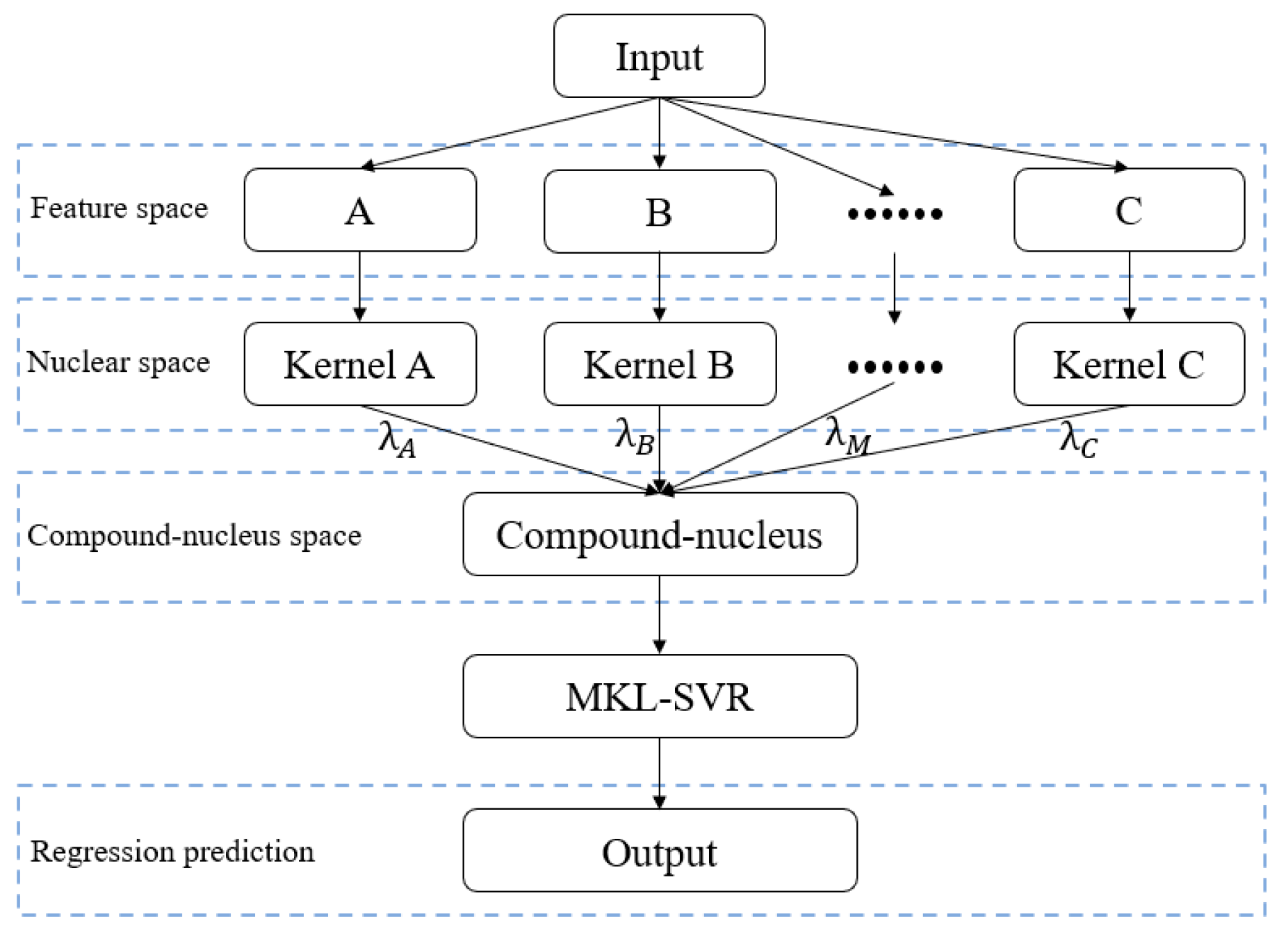
• To enhance the prediction accuracy of the model, we introduce a multi-kernel learning (MKL) method in conjunction with the traditional support vector regression approach. The SVR model is refined using Gaussian, polynomial, and sigmoid kernels to improve the precision and robustness of the model predictions.
• Using an in-depth analysis of components closely linked to sound insulation performance in the noise transmission path, we determine and sequentially correlate quantitative indices for the sound absorption and insulation of each component. Subsequently, we propose a prediction method for the sound insulation performance of the vehicle body system.
• In order to predict the interior noise performance of multi-frequency points under different working conditions at the same time, the single-kernel SVR and MKL-SVR methods are used to predict the interior noise of 17 one-third octave intervals.

This article is organized as follows: Section 2 provides an overview of the theoretical foundations of SVR and MKL-SVR. Section 3 introduces the decomposition architecture for predicting the sound insulation performance of the vehicle body system. Section 4 involves preprocessing the sample data post data enhancement. Section 5 provides a comprehensive summary of this paper’s content based on the conducted research.

2. The Multi-Kernel Learning–Support Vector Machine

2.1. A Brief Introduction to SVR

SVR is a machine learning regression method based on statistical learning theory [29]. For regression problems, the traditional approach is to calculate the error between the predicted value and the true value, measure it with the loss function, and obtain the prediction model by minimizing the loss function. The traditional linear regression method calculates the loss as long as the predicted value is not equal to the real value, and the support vector regression has a $ϵ$ (tolerance deviation; a manually set empirical value) between the predicted value and the real value. As shown in Figure 1, the red thick dotted line is a linear function, and the distance between the two red thin dotted lines and the middle red thick dotted line is $ϵ$. The green circles are the samples that fall into the interval band, and the black-edge circles are the samples that fall outside the interval band, also known as the support vector. SVR creates an ‘interval band‘ on both sides of the linear function and does not calculate the loss for all samples falling into the interval band. Only the support vector has an impact on the prediction function model. Finally, the optimized model is obtained by minimizing the total loss and maximizing the interval.

The sample data in the interval band does not affect the prediction function model, which shows an important property of the support vector regression method. After the training is completed, most of the training samples do not need to be retained, and the final model is only related to the support vector. Assume that there is a set of data sets R: $\{(x_1,y_1),(x_2,y_2),$ ……$,(x_n,y_n)\}$. The purpose of regression analysis is to learn a model $f\left(x\right)$ that can describe the relationship between $f\left(x\right)$ and $x$ as accurately as possible, and introduce $L_2$ regularization to describe the complexity of the model. Thus, SVR can be formalized as follows [30]:

$$\begin{array}{l}mi{n}_{w,b}\frac{1}{2}||w|{|}^2+C{\displaystyle \sum _{i=1}^n{l}_{\epsilon }(f(x_i)-y_i)}\\ l_{\epsilon }(z)=\{\begin{array}{l}0,|z|\le \epsilon \\ |z|-\epsilon ,|z|>\epsilon \end{array}\end{array}$$

(1)

where $w$ and $b$ are the normal vector and bias parameters of the model, respectively, C is the regularization parameter, $l_{\epsilon }\left(z\right)$ is the interval band-insensitive loss function, ε is the interval-band width, $\Vert w {\Vert }^2$ is the $L_2$ regularization term, which represents the model complexity, and the loss function term represents the model training error. C is used to balance the complexity of the model and the training error. The larger the C, the greater the proportion of the loss function term. The above minimization equation requires that C is as small as possible and that the loss function is as small as possible, that is, the training error of the model is as small as possible. The smaller the C, the larger the proportion of regularization terms and the lower the complexity of the model.

Linear regression usually belongs to ‘hard interval’ classification. This classification requires that each node must meet the constraints of the response. Therefore, the model is very sensitive to noise, and the points that do not conform to the law in the sample have a great influence on the results. In order to reduce the influence of these outliers on the results, the relaxation variables ${\mathsf{\xi }}_i$ and ${\mathsf{\xi }}_i^{*}$ are introduced into the SVR method, which makes the calculation of the loss function more flexible:

$$\begin{array}{l}mi{n}_{w,b,\epsilon }\frac{1}{2}||w|{|}^2+C{\displaystyle \sum _{i=1}^n{l}_{\epsilon }({\xi }_i+{\xi }_i^{*})}\\ s.t.\{\begin{array}{l}f(x_i)-y_i\le \epsilon +{\xi }_i\\ y_i-f(x_i)\le \epsilon +{\xi }_i^{*}\\ {\xi }_i,{\xi }_i^{*}\ge 0\end{array}\end{array}$$

(2)

where ${\xi }_i$ and ${\xi }_i^{*}$ are relaxation variables.

By introducing the Lagrange multiplier method, the above equation is further transformed into a dual problem:

$$\begin{array}{l}\max {\displaystyle \sum _{i=1}^n{y}_i(a_i^{*}-a_i)}-\frac{1}{2}{\displaystyle \sum _{i,j=1}^n(a_i^{*}-a_i)}(a_j^{*}-a_j)(x_i,x_j)-\epsilon {\displaystyle \sum _{i=1}^n(a_i^{*}+a_i)}\\ s.t.\{\begin{array}{l}{\displaystyle \sum _{i=1}^n(a_i-a_i^{*})=0}\\ 0\le a_i\le C\\ 0\le a_i^{*}\le C\end{array}\end{array}$$

(3)

where $a$ and $a^{*}$ are the Lagrange multipliers.

The Karush–Kuhn–Tucker (KKT) condition is a necessary condition for the optimal solution of nonlinear programming. The above process requires the KKT condition to be satisfied. Finally, the solution of SVR is calculated as follows:

$$f(x)={\displaystyle \sum _{i=1}^n(a_i-a_i^{*})(x_i,x_j)+b}$$

(4)

For nonlinear cases, it is necessary to use nonlinear mapping to project the data into a high-dimensional feature space (Hibert space) and use a linear classifier in the feature space. Because of the exponential growth in the dimension mapped to the high-dimensional space, it is difficult to calculate, so the kernel function is introduced. The kernel function first performs feature calculation in the low dimension and then expresses the actual classification results in the high dimension, which can effectively reduce the computational complexity while obtaining the correct results. The commonly used kernel functions are shown in

Table 1. Common kernel functions.

Name	Expression
linear kernel	K ($x_i, x_j$) = $x_i^T{x}_j$
polynomial kernel	K ($x_i, x_j$) =${\left(x_i^T{x}_j\right)}^d$
Gaussian kernel	K ($x_i, x_j$) = $e^{\left(-\frac{{||x_i-x_j||}^2}{2{\sigma }^2}\right)}$
sigmoid nucleus	K ($x_i,x_j$) = tanh ($\beta x_i^T{x}_j+\theta$)

. The kernel function is defined as:

$$K(x_i,x)=(\mathsf{\Phi }(x_i),\mathsf{\Phi }(x_j))$$

(5)

where Φ ($x$) is the transformation of variables from the original space to the high-dimensional feature space, and $i$ and $j$ refer to Equation (3).

By mapping the input variables to the high-dimensional feature space, linear regression is realized in the high-dimensional space. The solution of SVR is as follows:

$$f(x)={\displaystyle \sum _{i=1}^n(a_i-a_i^{*})}K(x_i,x_j)+b$$

(6)

2.2. Introduction to MKL-SVR Theory

With the deepening of mechanism research in recent years, the application of the kernel function has improved the algorithm and greatly expanded the application of related algorithms in text classification, image recognition, disease diagnosis, financial risk control, and other fields [31]. The processing effect of the SVR model is closely related to the selection of the kernel function. The traditional support vector regression method usually chooses a single kernel function. However, for complex problems such as large sample sizes, irregular multidimensional data, and an uneven distribution, it is limiting to use a single kernel function for processing. In this regard, multiple kernel functions can be combined, and the optimal linear combination of multiple kernels can be used to replace the single kernel to obtain better model performance, that is, the so-called Multiple Kernel Learning method [32].

MKL is widely used in different fields as a feature selection technique. It can be a combination of different parameters of the same kernel function or a combination of different kinds of kernel functions. Each kernel function may use different features to describe the features from different data sources. Therefore, the optimization problem of the original model is transformed into the selection problem of kernel weight λ. Figure 2 shows the learning process of the MKL-SVR model.

The weighted kernel [33,34] is constructed as follows:

$$\begin{array}{l}K(x_i,x_j)={\displaystyle \sum _{l=1}^n{\lambda }_l}{K}_l(x_i,x_j)\\ \lambda \ge 0,{\displaystyle \sum _{l=1}^n{\lambda }_l=1}\end{array}$$

(7)

where $\lambda$ is the weight coefficient, and the $i$ and $j$ values refer to Equation (3).

Substituting the weighted kernel obtained in Equation (7) into Equation (6), the final solution of MKL-SVR is as follows:

$$f(x)={\displaystyle \sum _{i=0}^n(a_i-a_i^{*}){\displaystyle \sum _{l=1}^n{\lambda }_l{K}_l(x_i,x_j)}+b}$$

(8)

where the parameters refer to Equation (3).

The solution of the application of the known method for acoustic problems in cars is that MKL-SVR adds a weighted kernel based on the SVR solution, and the sum of kernel weights is 1. Therefore, the solution of the newly constructed MKL-SVR can flexibly select different features of different kernel functions to describe the characteristics from different data sources, thus avoiding the limitations of using a single kernel function to process data.

3. Experimental Test and Data Collection

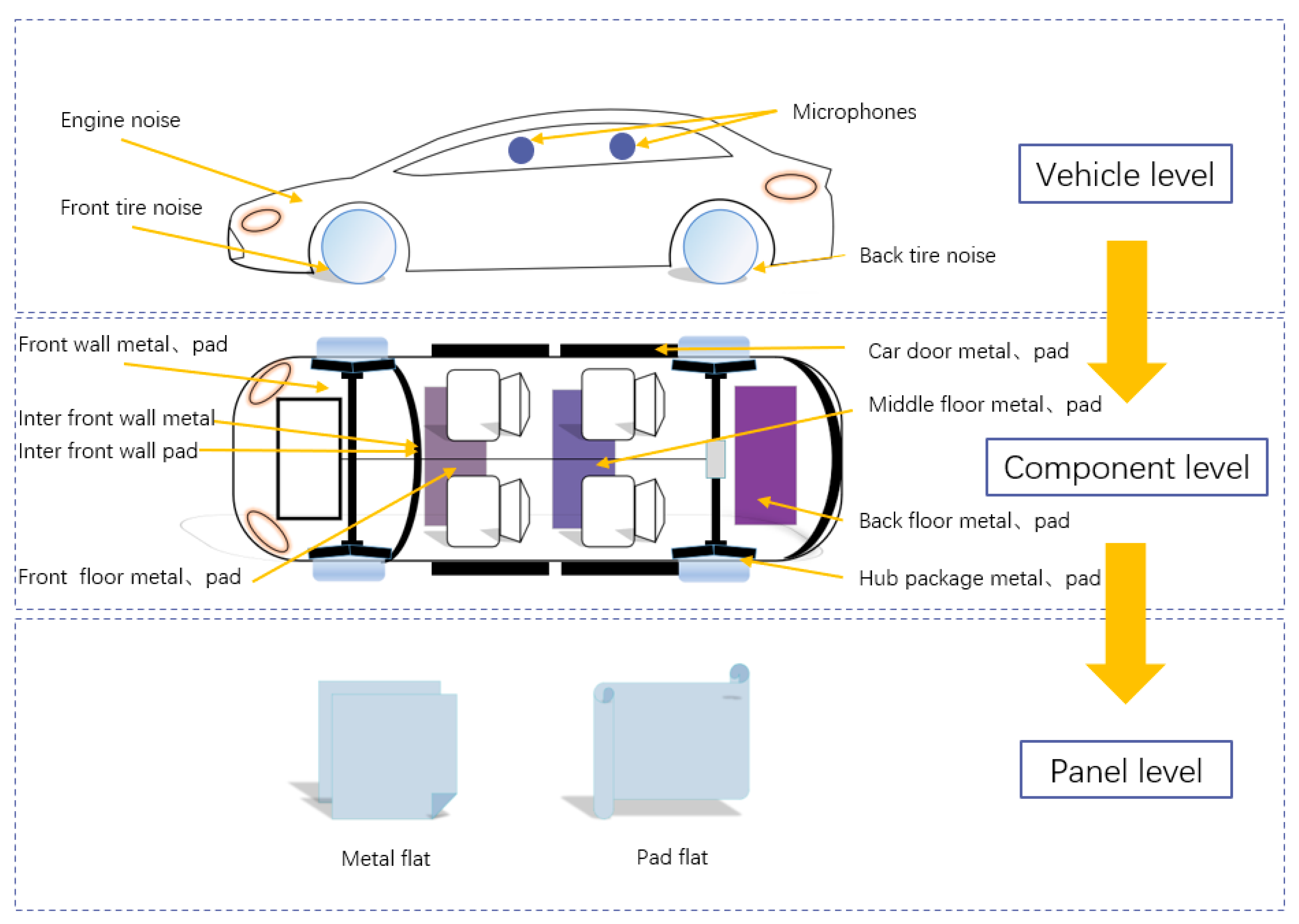
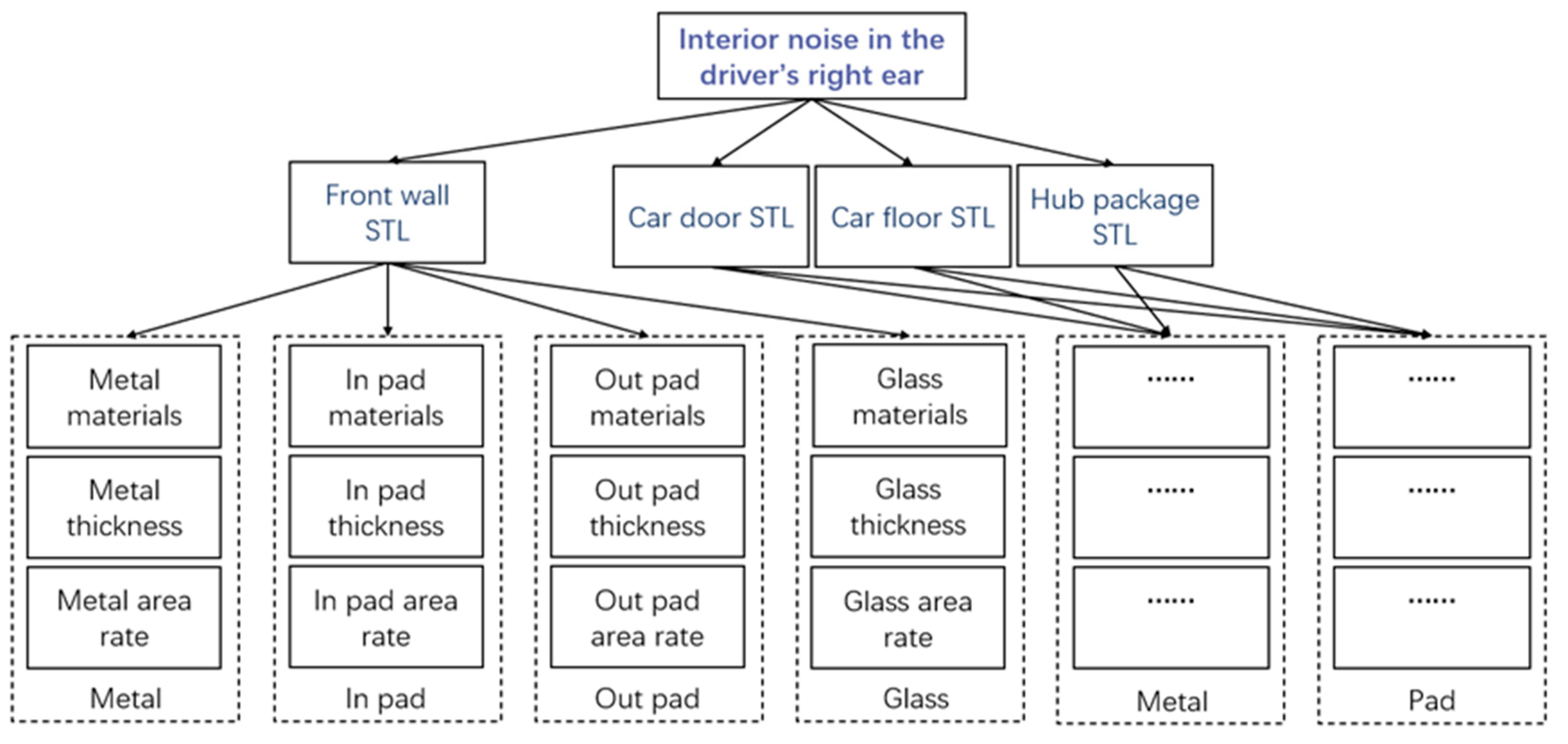
3.1. Analysis Method for Sound Insulation Performance of the Car Body System

At present, interior noise is mainly controlled by applying acoustic packets on the noise transmission path. The acoustic package component is a multi-layer composite packaging structure with sound absorption and sound insulation performance [35]. Multiple acoustic packages are arranged in the front of the car, the door, the front, middle and rear floor carpets of the car floor, the car wheel hub package and other locations, which improves the sound insulation performance of the car body system. At the same time, the sound insulation problem of the body system becomes a comprehensive problem involving many unit components. Therefore, the analysis of the sound insulation performance of the body cannot only focus on the top-level performance indicators; it must also analyze the sound absorption and sound insulation performance of the unit components that make up the body system [36]. Hierarchical decomposition is an analytical method that combines theoretical analysis and practical engineering experience. By decomposing the overall technical indicators into components step by step, the design influencing factors hidden under the hierarchy are found [37]. The premise is to reveal the quantitative relationship between the related unit indicators in the hierarchical system. The prediction of the sound insulation performance of the vehicle body system must rely on the analysis of the noise transmission path in the vehicle to define the unit components closely related to the sound absorption and insulation performance of the vehicle body system. According to the order of ‘vehicle level’, ‘component level’, and ‘panel level’, the quantitative indexes of the sound absorption and insulation performance of each level unit are determined and correlated from top to bottom, and the decomposition framework of the sound insulation performance prediction of the vehicle body system is established. The vehicle level represents the path sound insulation performance: the noise source to the noise attenuation of the receiving point. The component level represents the sound absorption and insulation performance of the sheet metal and sound insulation pad of the front, door, floor and hub package. The panel level represents the sound absorption and insulation performance of the sheet metal and sound insulation pad of each plate, as shown in Figure 3.

According to the specific attributes of the prediction problem, this paper analyzes the propagation mechanism of the air sound in the vehicle dominated by ‘tire noise’. Accordingly, the quantitative relationship between the related indexes in the hierarchical decomposition system can be explored, and the sound insulation performance of the body system can be predicted step by step from bottom to top [38]. Among them, the hierarchical decomposition of the sound insulation performance of the front system for vehicle tire noise can be characterized as shown in Figure 4. The front panel system includes the front panel sheet metal, the inner front panel sound insulation pad, the outer front panel sound insulation pad, and the front windshield. The next level legend of the front panel system includes the sheet metal material, thickness, and area ratio; the material, thickness, and area ratio of the inner sound insulation pad; the material, thickness, and area ratio of the outer sound insulation pad; and the material, thickness, and area ratio of the front windshield. The hierarchical decomposition of the door, floor, and hub package is similar to the decomposition of the front wall system. According to the hierarchical decomposition of the sound insulation performance of the vehicle sound system, the sound insulation performance test was carried out, including the sound insulation test of the whole vehicle, the sound insulation test of the components, and the sound insulation test of the plate. The sound absorption performance test was also carried out, including the component sound absorption test and the plate sound absorption test.

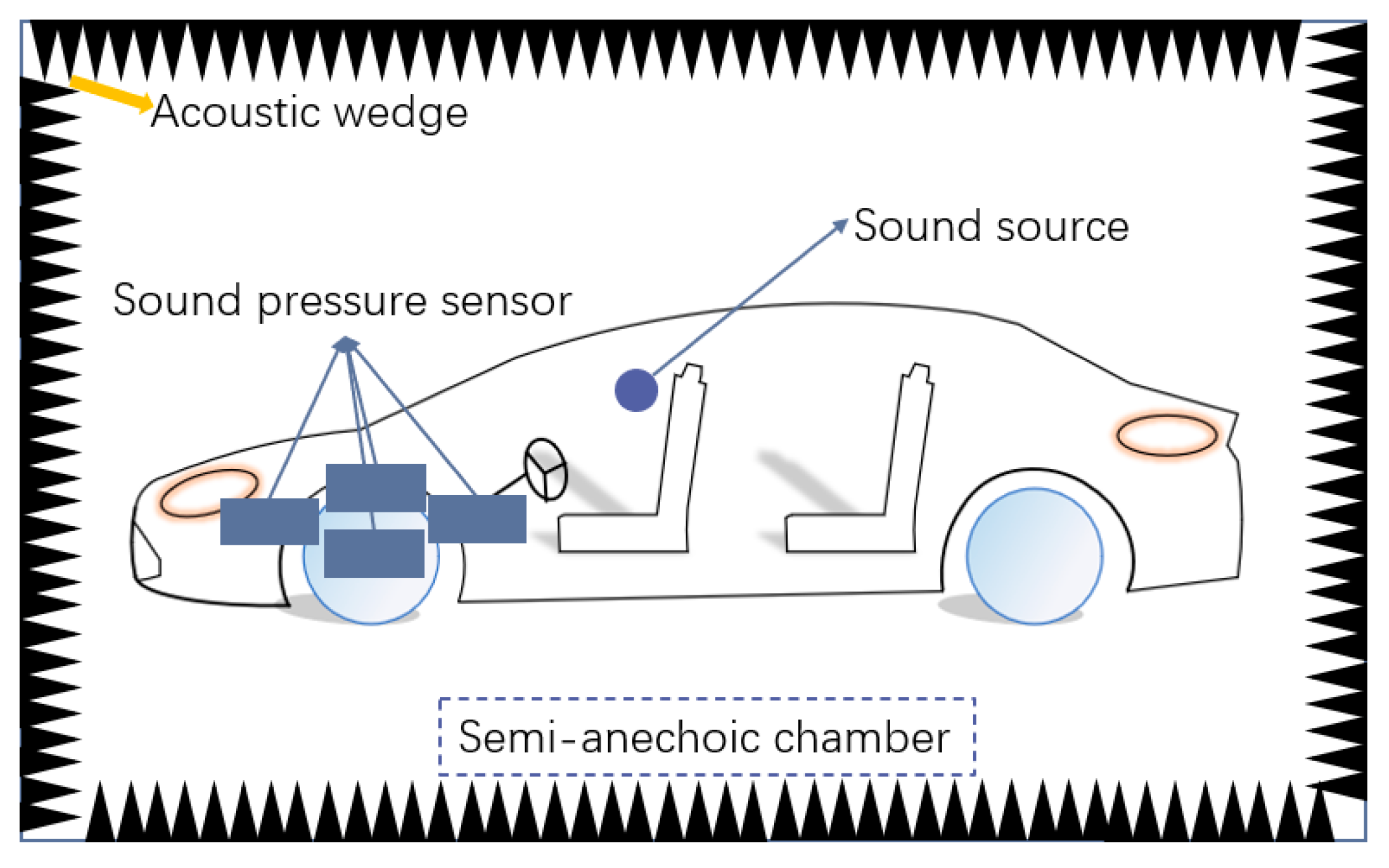
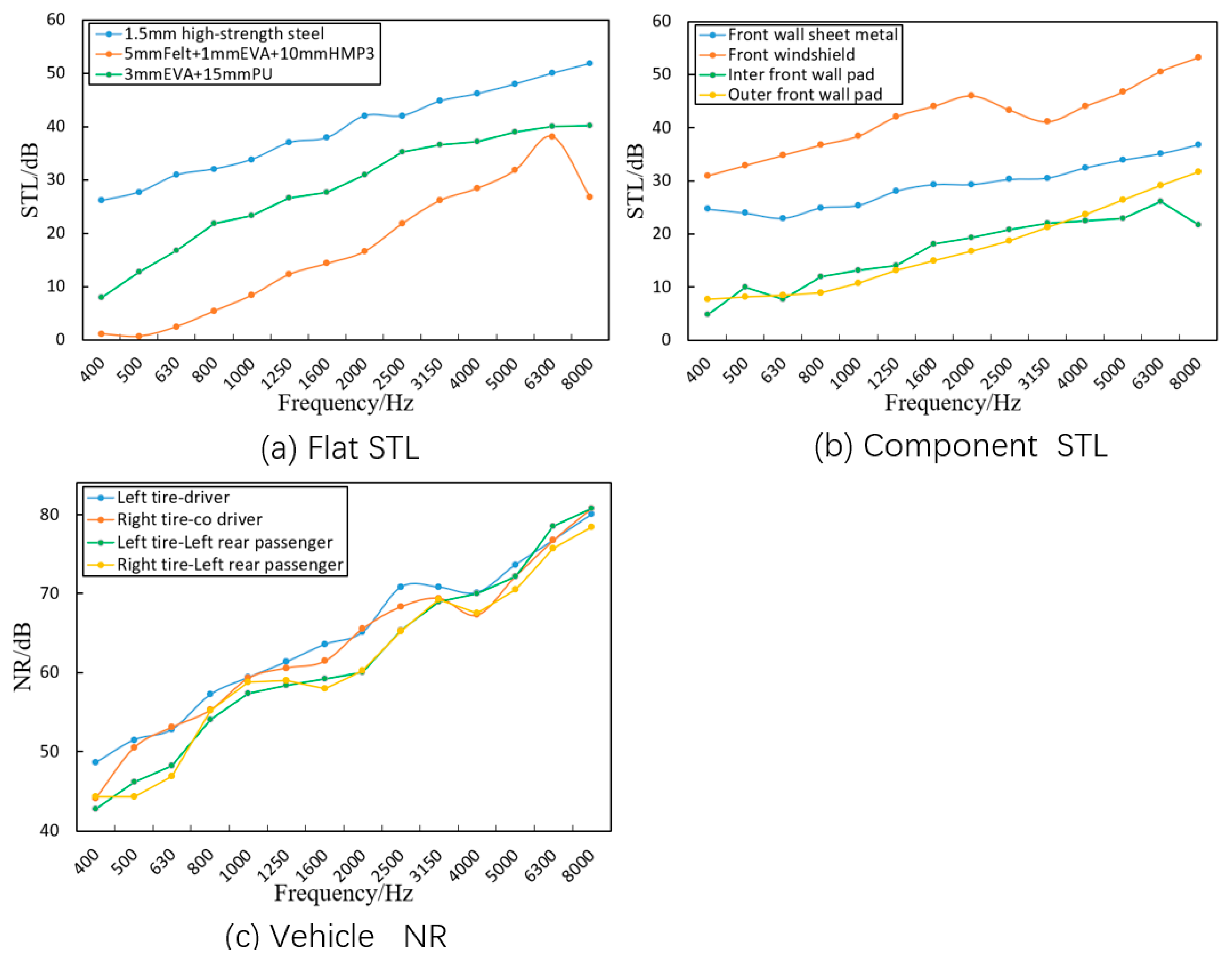
3.2. Sound Insulation Performance Test

The acoustic performance is reflected in the sound field, and it is also measured in the sound field [39]. In order to test the sound insulation performance of structural parts, relevant sound insulation data are collected to support the construction of prediction models and ultimately help enterprises and factories to plan early in the design, improve efficiency, and reduce costs. The sound insulation performance test involves carrying out a real vehicle test on a certain model of an enterprise and collecting data to build a sound insulation performance prediction model. In order to collect enough data to reflect the mapping relationship between the parameters of the acoustic package and the interior noise of different frequencies, a variety of different combinations of acoustic package schemes were introduced into the experiment. According to decomposition, the sound insulation performance of the test vehicle was tested at the plate level, component level, and vehicle level, and the relevant noise data were collected. When sound waves are incident on the surface of acoustic materials, sound insulation structures, and sound insulation packaging, part of the incident sound energy is reflected back by the surface of the material, and the other part of the incident sound energy continues to propagate in the air or medium through the sound insulation material. Comparing the transmitted sound energy with the incident sound energy, the smaller the transmitted sound energy, the greater the sound transmission loss, as shown in Figure 5. Sound transmission loss (STL) is an index used to measure the sound insulation capacity of materials. The greater the STL, the better the sound insulation performance of materials. The calculation equation of transmission loss is expressed as:

$$\tau =\frac{E_{\mathrm{t}}}{E_{\mathrm{i}}}$$

(9)

$$STL=10\log (\frac{1}{\tau })=10\log E_{\mathrm{i}}-10\log E_t$$

(10)

where $\tau$ is the acoustic transmission coefficient, which is the ratio of the transmitted acoustic energy to the incident acoustic energy, $E_i$ is the incident acoustic energy, and $E_t$ is the transmitted acoustic energy.

According to the standard GB/Z27764-2011 ‘Acoustics: Measurement of sound transmission loss in impedance tube-Transmission matrix method (four microphone method)’, the sound insulation performance test was carried out using a standing wave tube [40]. First, the impedance tube was installed on the test bench to connect the noise source sound. Then, the impedance tube, GRAS.32 sound pressure sensor, and SIEMENS SCADAS Mobile test equipment were connected in order. After connecting the PC terminal with the test equipment, the LMS.Testlab software 2021 was used to perform channel setting, sensitivity calibration, and phase-amplitude calibration. The sample was loaded into the impedance tube to carry out the sound insulation performance test of the plate.

The sound insulation performance of the components was measured with the transmission loss. According to the standard ISO15186-1-2003 ‘acoustic intensity is used for sound insulation measurement of buildings and building components’, the ‘reverberation chamber-semi-anechoic chamber window’ test was carried out [41]. The measured sample was installed in the window, the sound source was placed in the reverberation chamber as the sound chamber, and the sound pressure sensor was arranged in the reverberation chamber to measure the sound pressure level in the reverberation chamber. The semi-anechoic chamber was used as the receiving chamber, and the sound intensity level was measured with the sound intensity probe. According to Equations (9) and (10), the transmission loss of plates and components was calculated.

The sound insulation performance of the vehicle uses the noise attenuation (NR) from the noise source to the receiving point as the performance evaluation index. The noise attenuation is used to describe the propagation path, that is, the sound wave attenuation from the noise source to the receiving point. The vehicle sound insulation test is shown in Figure 6. The test vehicle was placed in a semi-anechoic room. In order to better simulate the sound transmission process, the noise sources at the noise receiving point were exchanged (that is, the volume sound source was arranged at the noise receiving point, and the sound pressure sensor was arranged at the noise source position). Four sound pressure sensors were arranged on the front, rear, left, and right sides of the four tires of the car, and the right ear side of the driver or passenger closest to each wheel was used as the noise receiving point for testing and data collection. Equation (11) was used to calculate the noise attenuation of the vehicle.

$$NR=SP{L}_{\mathrm{s}}-SP{L}_{\mathrm{r}}$$

(11)

where $SP{L}_S$ is the sound pressure level of the sound source and $SP{L}_r$ is the sound pressure level of the receiving point.

Using the above test methods, the sound insulation performance tests of various flat parts, components, and vehicles were carried out. In Figure 7, the sound insulation performance test data of some flat parts, components, and vehicles are shown.

The plate-level sound insulation performance test tests the flat plates of different materials and thickness combinations. The transmission loss of a flat plate of a specific material and thickness combination is measured with an impedance tube test. The green curve in (a) is the transmission loss of the combined flat plate of the EVA plate with a thickness of 3 mm and the PU plate with a thickness of 15 mm. The component-level sound insulation performance test tests different components and measures the transmission loss of each component using the ‘reverberation chamber-semi-anechoic chamber window’ test. The green curve in (b) is the transmission loss of the inner front enclosure sound insulation pad measured with the test. The vehicle-level sound insulation test tests different paths and measures the noise attenuation of a certain path by placing the real vehicle in a semi-anechoic chamber. The green curve in (c) is the noise attenuation during the transmission process of the left rear wheel-left rear passenger.

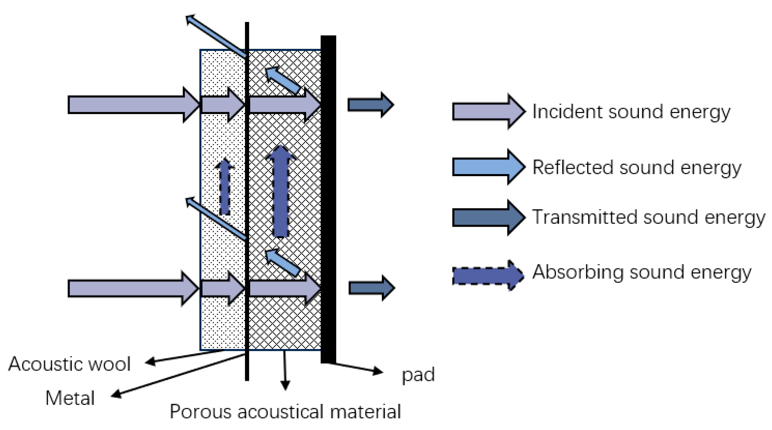
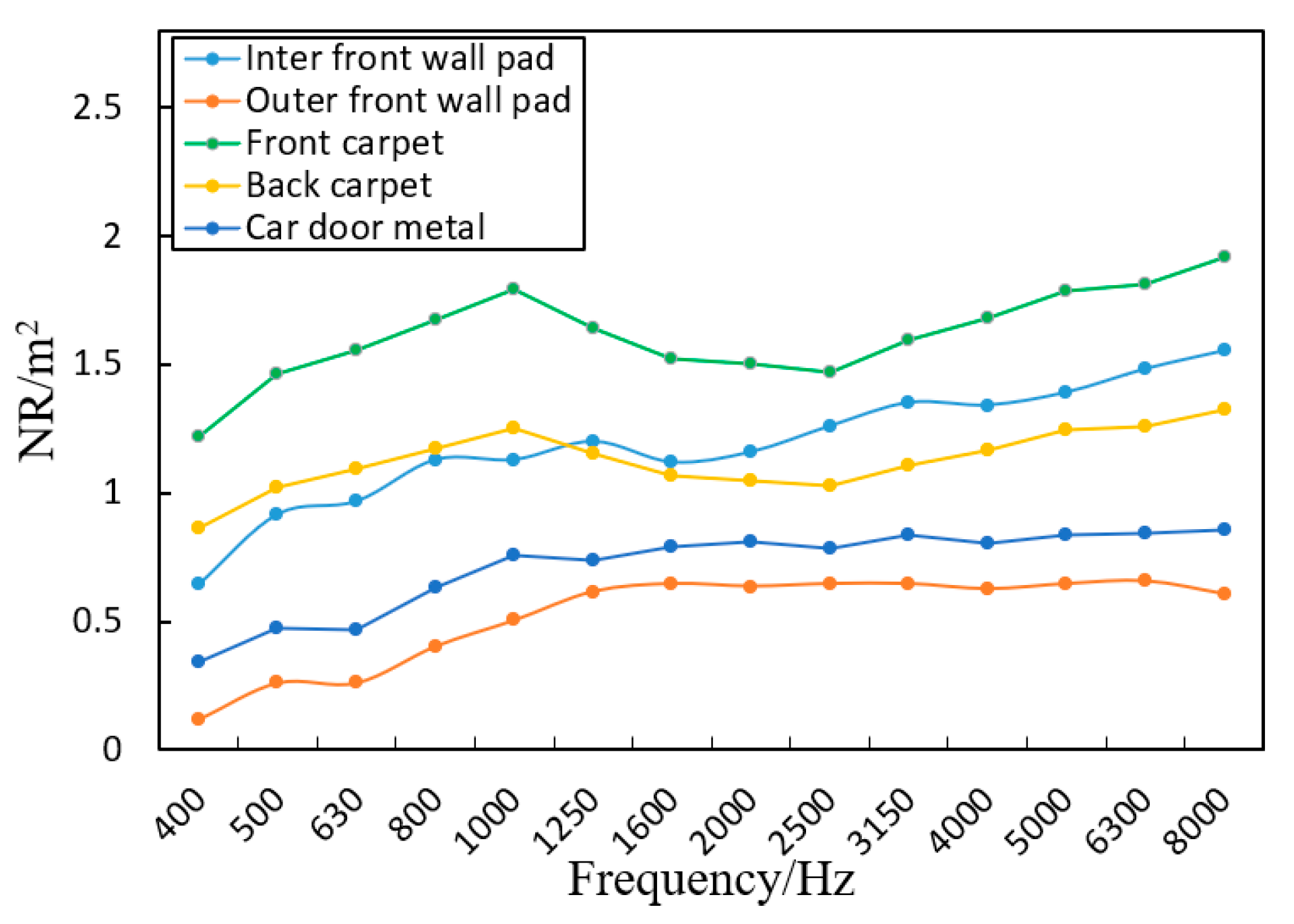
3.3. Sound Absorption Performance Test

The sound absorption performance also reflects the sound insulation performance of the vehicle body. Therefore, it is necessary to build a sound absorption performance prediction model for related research. In order to obtain the mapping relationship between the sound absorption performance of different body system structures and the interior noise at different frequencies, the sound absorption performance test is designed to collect sufficient data to analyze the above relationship. When the incident sound energy reaches the sound insulation material, the sound insulation structure, and the sound insulation packaging surface, in addition to the reflected sound energy and the transmitted sound energy, there is also a part called the absorbed sound energy, as shown in Figure 5 in Section 3.2. The realization of the sound absorption process is the transmission process of the sound wave emitted by the sound source in the medium. The friction force generated by the interaction between the air and the sound wave causes a part of the sound wave energy to be converted into heat energy, and the sound energy is reduced. At the same time, the heat exchange and heat conduction between the air and medium will also lead to a reduction in sound energy. The materials used for sound-absorbing components are generally porous sound-absorbing materials. The sound absorption coefficient is used to measure the ability of sound-absorbing materials. It is defined as the ratio of absorbed energy to incident energy. The expression is as follows:

$$\alpha =\frac{E_a}{E_i}=1-\frac{E_r}{E_i}$$

(12)

where $\alpha$ is the sound absorption coefficient, $E_a$ is the absorbed sound energy, $E_i$ is the incident sound energy, and $E_r$ is the reflected sound energy.

In practical engineering applications, the sound absorption coefficient of the material is usually calculated with the reverberation test using the Sabine equation:

$$\alpha =\frac{0.163V}{S}(\frac{1}{T_2}-\frac{1}{T_1})+{\alpha }_1$$

(13)

where $V$ is the volume of the test device, $T_1$ and $T_2$ are the reverberation time before and after the specimen is placed, respectively, $S$ is the area of the specimen, and $a_1$ is the average sound absorption coefficient of the reverberation chamber.

In order to facilitate the analysis, when the equation is used in the test, the main test is the sound absorption capacity of the material per unit area of the measured part. In the automotive industry, the sound absorption capacity is usually used to measure the sound absorption capacity of different materials in different areas. The sound absorption calculation equation is the product of the sound absorption coefficient and the area of the material used, as shown in Equation (14):

$$A=\alpha \times S$$

(14)

where $\alpha$ is the sound absorption coefficient and $S$ is the specimen area.

The sound absorption performance of the components and the plate was tested with the reverberation chamber method. The density of each point in the reverberation chamber is evenly distributed, and the acoustic phase in each direction is randomly and irregularly distributed. The above method was used to test the sound absorption performance of plates and components. Figure 8 shows the measured sound absorption performance data of some plates and components.

By bringing the parameters and results of the sound absorption performance test into the formula, the sound absorption coefficient and sound absorption amount were calculated, so as to calculate the noise attenuation during the sound absorption test of the components and flat parts. In Figure 8, the green curve is the noise attenuation of the front carpet sound insulation pad, the yellow curve is the noise attenuation of the rear carpet sound insulation pad, and the orange curve is the noise attenuation of the outer front sound insulation pad.

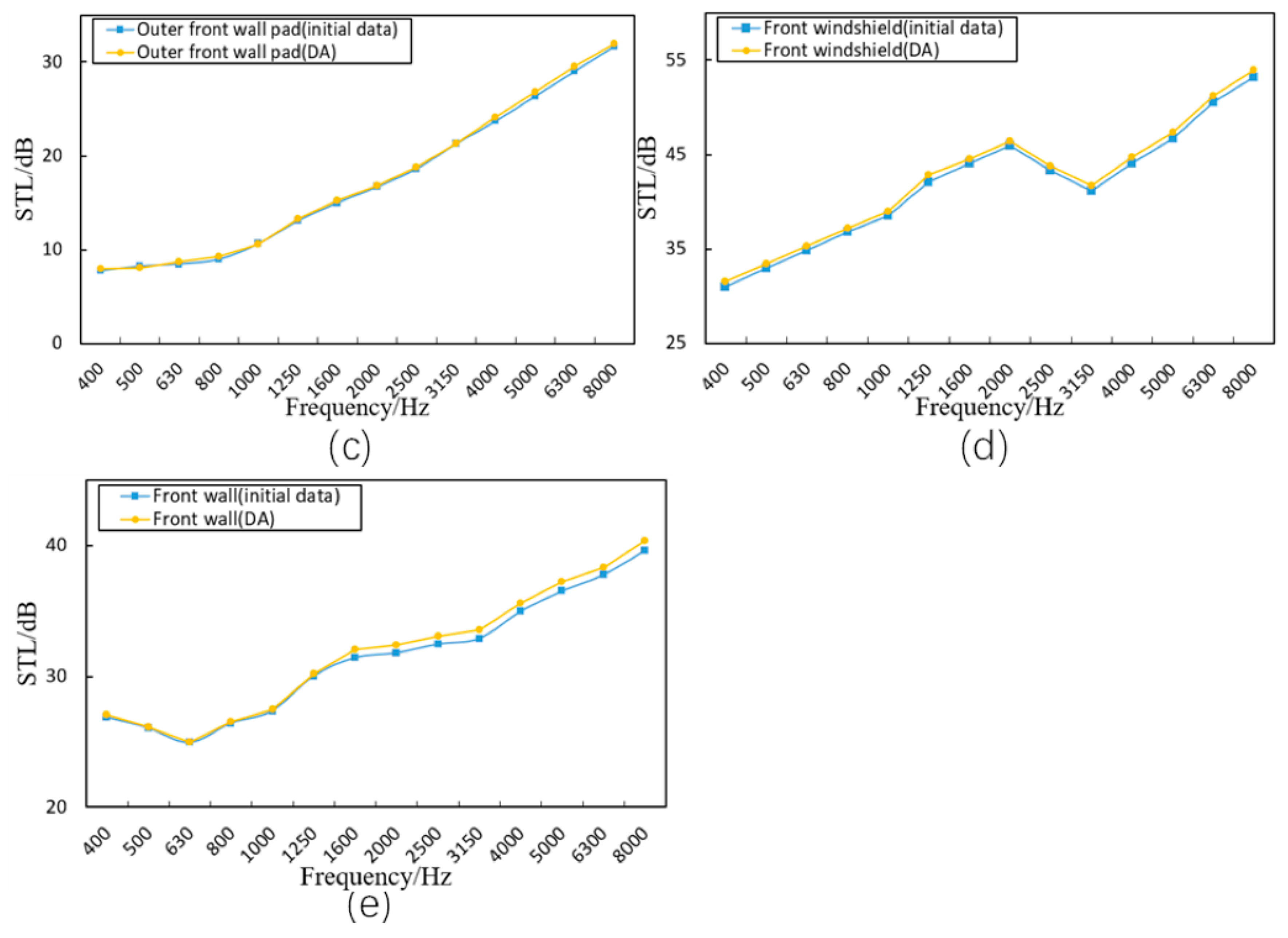
3.4. Data Augmentation

Based on the test method, a total of 15 groups of body acoustic package sound absorption and insulation samples were collected. One group of front system sample information is shown in

Table 2. The original data of sound insulation performance of a group of samples in the front system.

Frequency (Hz)	Front Wall STL (dB)	Front Wall Sheet Metal STL (dB)	Inter Front Wall Pad STL (dB)	Outer Front Wall Pad STL (dB)	Front Windshield STL (dB)
400	25.85	24.68	4.84	7.74	30.97
500	28.63	23.95	9.92	8.23	32.90
630	32.16	22.98	7.74	8.47	34.84
800	34.68	24.92	11.85	8.95	36.77
1000	36.42	25.40	13.06	10.65	38.47
1250	38.12	28.06	14.03	13.06	42.10
1600	40.28	29.27	18.15	15.01	44.03
2000	41.90	29.27	19.35	16.69	45.97
2500	43.59	30.24	20.81	18.63	43.31
3150	45.98	30.48	22.02	21.29	41.13
4000	48.43	32.42	22.51	23.71	44.03
5000	50.34	33.87	22.98	26.37	46.69
6300	51.72	35.08	26.13	29.03	50.56
8000	51.92	36.77	21.77	31.69	53.23

, and other system information is similar. The number of sample data obtained from the experiment was not enough to obtain a good training model and prediction results. The existing data set was expanded using DA (Data Augmentation) [42,43], adding random noise, random fluctuations, etc., to generate some extended data containing the existing data features, thereby increasing the number of samples, eliminating the common machine learning problem of over-fitting caused by a small data set training model [44], and improving the model effect and prediction results.

The Mixup enhancement algorithm in many DA methods is introduced in [45,46]. This method is widely used in many general fields because of its simple and effective characteristics. The main idea of the Mixup method is to transform the empirical Dirac distribution into an empirical domain distribution and use linear interpolation to mix two different samples and sample labels in the original data set to generate a new sample. The sample set size and training data distribution space are expanded without adding new sample size, thereby improving the generalization ability of the model. In this paper, the above Mixup method was used to enhance the data. Two different data were randomly selected from the original sample data set, and then a new sample was calculated and generated using the randomly selected data, so as to expand the original data samples to 56 groups:

$$\begin{array}{l}\tilde{x}=\lambda x_i+(1-\lambda )x_j\\ \tilde{y}=\lambda y_i+(1-\lambda )y_j\end{array}$$

(15)

where $x$ and $x_i$ are data samples, $y$ and $y_i$ are the labels corresponding to the sample (the labels are all one-hot labels), and $x$ $\ne$ $y$, ($x_i$, $y_i$) and ($x_j$, $y_j$) are two data sets, ($\tilde{x}$, $\tilde{y}$) is a new data sample, and the random number $\lambda$ $\in$ [0, 1] and obeys the beta ($\alpha , \beta$) distribution. The function of hyperparameter $\alpha$ is to control the intensity of interpolation: the greater the value, the greater the intensity of interpolation. The value of $\alpha =\beta$ in this paper is 2.

Figure 9 is a comparison chart between a set of data enhancement samples and the original samples. A set of front data includes five groups of samples: front system, front sheet metal, inner front sound insulation pad, outer front sound insulation pad, and front windshield. The data augmentation in this paper obeys the beta distribution (α $=$ β $=$ 2), λ $\in$ [0, 1]. The smaller the λ value, the larger the sample data generated with interpolation, and vice versa. The closer the two sets of randomly selected sample data values are, the closer the new data generated with the Mixup method is to the original sample value. As (a) the front sheet metal data enhancement sample and the original sample comparison diagram shows, the new data generated with data enhancement is consistent with the overall trend in the original data, but there is no (c) external sound insulation pad data enhancement sample in the original sample comparison diagram. The effect is good, probably because (b) the two groups of samples randomly selected are compared with (a) the two groups of samples randomly selected and (b) the data values of each frequency point of the two groups of samples are closer.

4. Application and Validation of the Proposed Method

4.1. Data Pre-Processing

In order to eliminate the influence of data units and magnitudes and speed up the convergence of the training network, at the same time, because the model limits a certain range of output data, the input data needs to be normalized to the [0, 1] interval. The prediction model processes the input normalized data, and the prediction result is inversely normalized to the original magnitude data. The normalized equation is shown in Equation (16):

$$\mathrm{y}=(y_{\max }-y_{\min })\times \frac{x-x_{\min }}{x_{\max }-x_{\min }}+y_{\min }$$

(16)

where $x$ is the original data set, $x_{max}$ is the maximum value of the data set, $x_{min}$ is the minimum value of the data set, $y_{max}$ is the upper limit of the normalized interval; in this paper, we take 1, and $y_{min}$ is the lower limit of the normalized interval; in this paper, we take 0.

When importing data sets into the prediction model, it is necessary to divide the data sets into training sets and test sets. The model is trained using the data in the training set, so that the model can learn and explore the rules and relationships among the data pieces in this part. After the model training is completed, the remaining test set data from the training model is imported into the model, and the prediction results of the test set are analyzed to measure the prediction effect of the model. In this paper, the collected data sets are divided according to the ratio of the training set to the test set of 4:1. Among them, 45 groups of data sets are used for model training, 10 groups are used for model testing, and 1 group is used for model final verification.

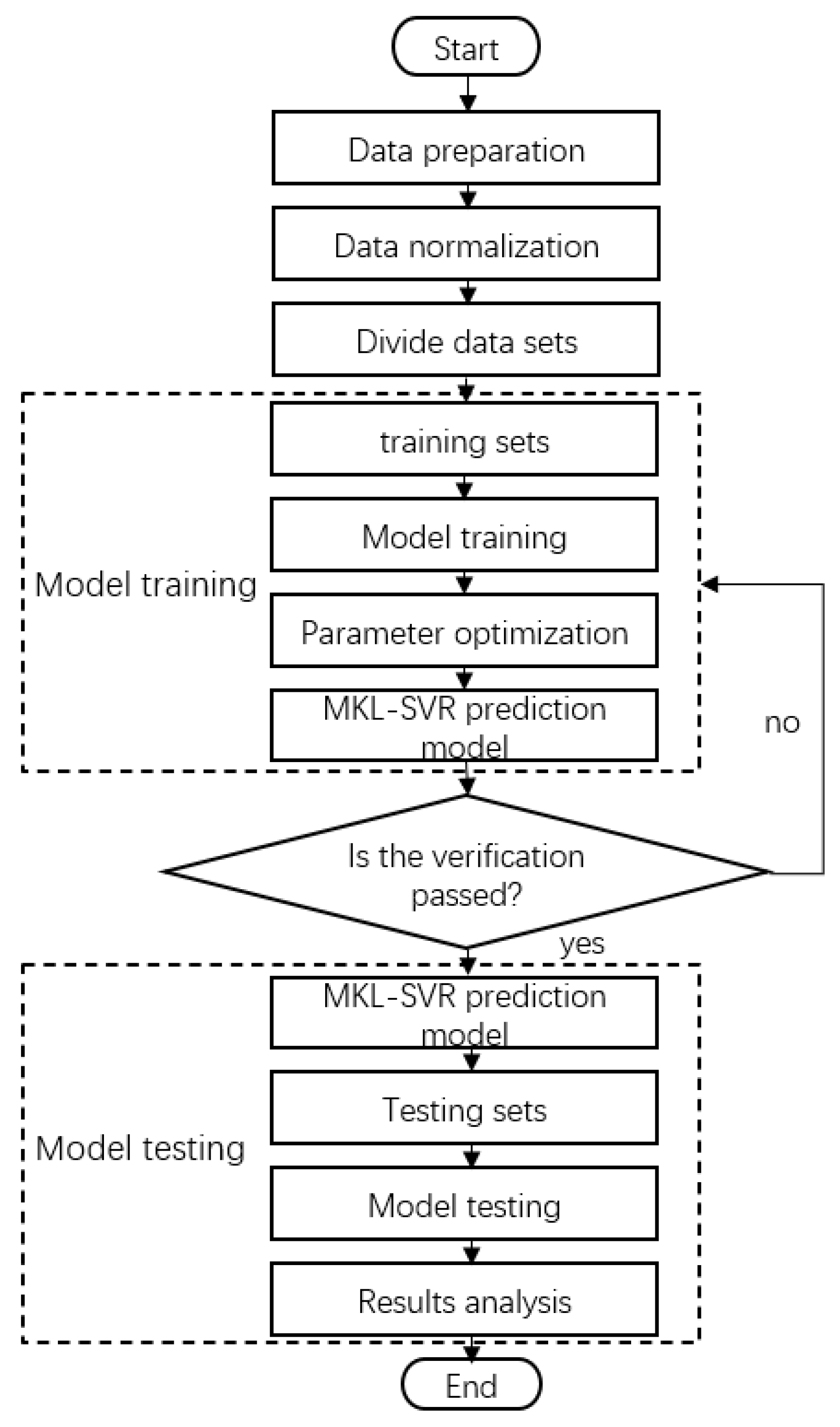
4.2. Establishing the Prediction Model of Sound Insulation Performance of the MKL-SVR Model

By testing the flat parts, components, and vehicles under different working conditions, accurate interior noise data are obtained. According to the Mixup method, the sample data are expanded and improved. Based on the decomposition system, the MKL-SVR method is introduced to analyze the engineering application problems, that is, the forward development model of sound insulation performance of the vehicle body system is analyzed and studied. When building the hierarchical model, the material, thickness area ratio, and the sound insulation corresponding to the 14 one-third octaves of the third-level plate-level sheet metal and sound insulation pad are taken as input, and the component-level transmission loss corresponding to the plate level is taken as output. When building the second level to the first level, the second-level components are used as the input of the model, and the first-level interior noise (interior noise at the driver’s right ear, interior noise at the co-driver’s right ear, interior noise at the left rear passenger’s right ear, and interior noise at the right rear passenger’s right ear) is used as the output of the model.

According to the hierarchical decomposition diagram of the body system shown in Figure 4 in Section 3.1, the quantitative relationship between the underlying element indicators and the adjacent intermediate-level elements, as well as the quantitative relationship between the intermediate-level element indicators and the adjacent top-level element indicators, are established, respectively. According to the quantitative relationship between the levels, numerical modeling is performed, as shown in Equation (17). Whether the $f_k^{\left[L\right]}$ prediction model is accurate or not affects the quality of the result prediction:

$$\begin{array}{l}{y}_k^{([L])}=f_k^{([L])}(x_1^{([L+1])},x_2^{([L+1])},\mathrm{...},x_R^{([L+1])}),k=1,2,\mathrm{...},K,L=1,2,\mathrm{...},L_0\\ s.t.\{\begin{array}{l}{c}_m^{([L])}(x^{([L])})\le 0,m=1,2,\mathrm{...},M\\ g_n^{([L])}(x^{([L])})\le 0,n=1,2,\mathrm{...},N\end{array}\\ \mathrm{var}.\{\begin{array}{l}{x}_r^{[L+1]}\in X_{\mathrm{r}}^{[L+1]},\mathrm{r}=1,2,\mathrm{...}R,R_1,\mathrm{...}{R}_2,\mathrm{...}{R}_3,\mathrm{...},R\\ y_k^{([L])}\in Y_k^{([L])}\end{array}\end{array}$$

(17)

where $L_0$ is the number of layers in the hierarchical decomposition system, $L$ is the calculation layer, $k$ is the number of elements in the corresponding level, $y_k^{\left[L\right]}$ is the design goal of the $k$th element in the $L$ layer, $f_k^{\left[L\right]}$ is the prediction model of the $k$th design goal in the $L$ layer, $x_r^{\left[L+1\right]}$ is the $r$th design variable in the $L+1$ layer, $X_r^{\left[L+1\right]}$ and $Y_k^{\left[L\right]}$ are the feasible region intervals of the $r$th design variable and the $k$th design variable in the $L+1$ layer and the $L$ layer, and $c_m^{\left[L\right]}$ and $g_n^{\left[L\right]}$ are the constraints of the numerical relationship equation.

At the same time, the MKL-SVR model is introduced to predict the sound insulation performance of the vehicle body system. The kernel function of the MKL-SVR model is the weighted kernel of the Gaussian kernel function, the polynomial kernel function, and the sigmoid kernel function. Because the prediction effect of the Gaussian kernel function model in each common kernel function is better, the kernel function of the single-kernel SVR model uses the Gaussian kernel function. The parameter configuration of the MKL-SVR and SVR models is shown in

Table 3. The predictive model configuration.

Configuration	Parameter
learning mode	single-core learning	MKL-SVR
number of training sets/validation sets	45/10	45/10
kernel function	Gaussian kernel function	Gaussian kernel function, polynomial kernel function, sigmoid kernel function
cross validation mode	five-fold cross validation	five-fold cross validation
parameter optimization method	grid search	grid search
parameter optimization range	c, g $\in$ ($2^{-10},2^{-10}$)	r, c, g $\in$ ($2^{-10},2^{-10}$), $d\in$(1,8), $\lambda \in$(0,1)

. The training and testing process of the MKL-SVR model and the SVR model is shown in Figure 10.

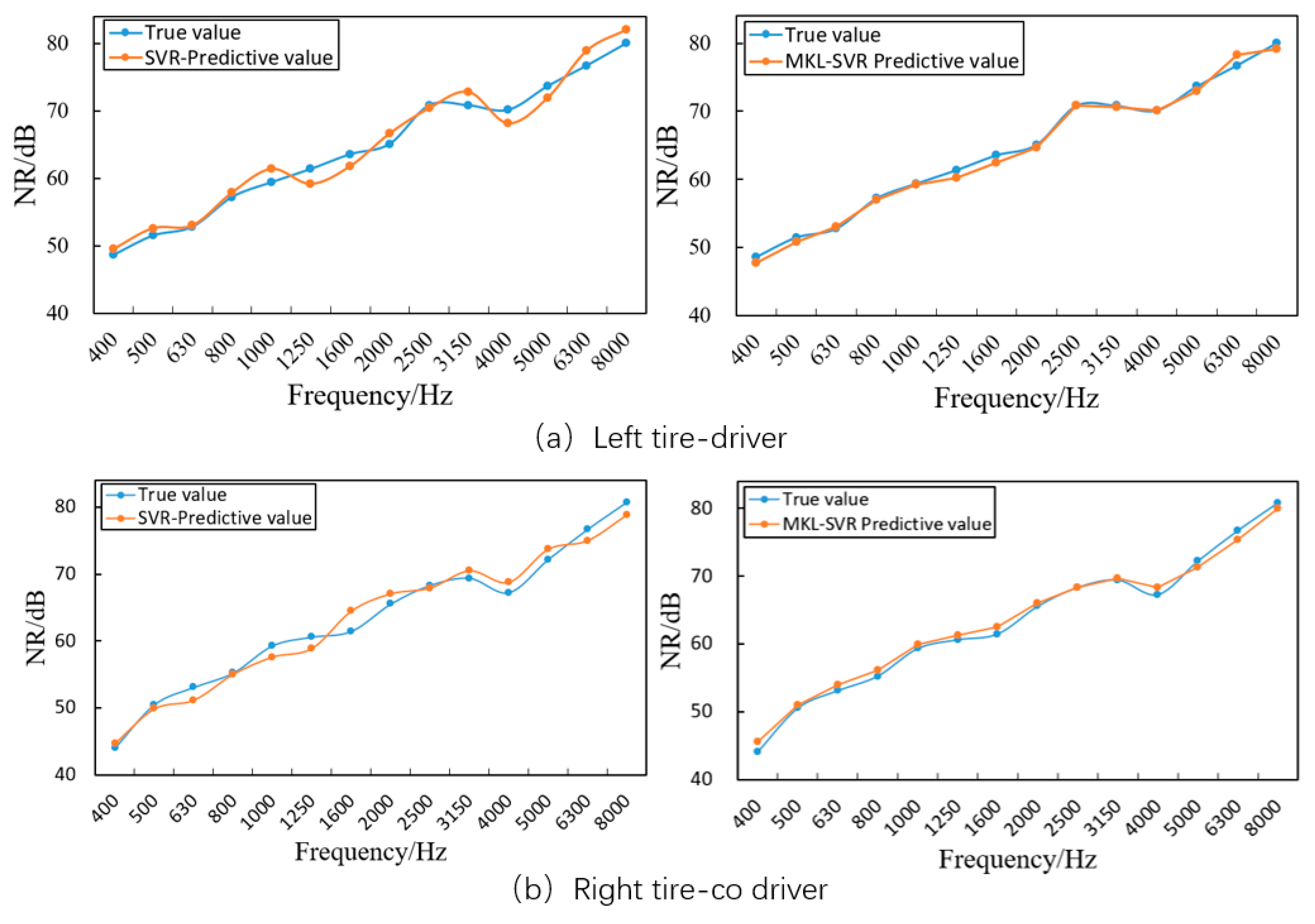
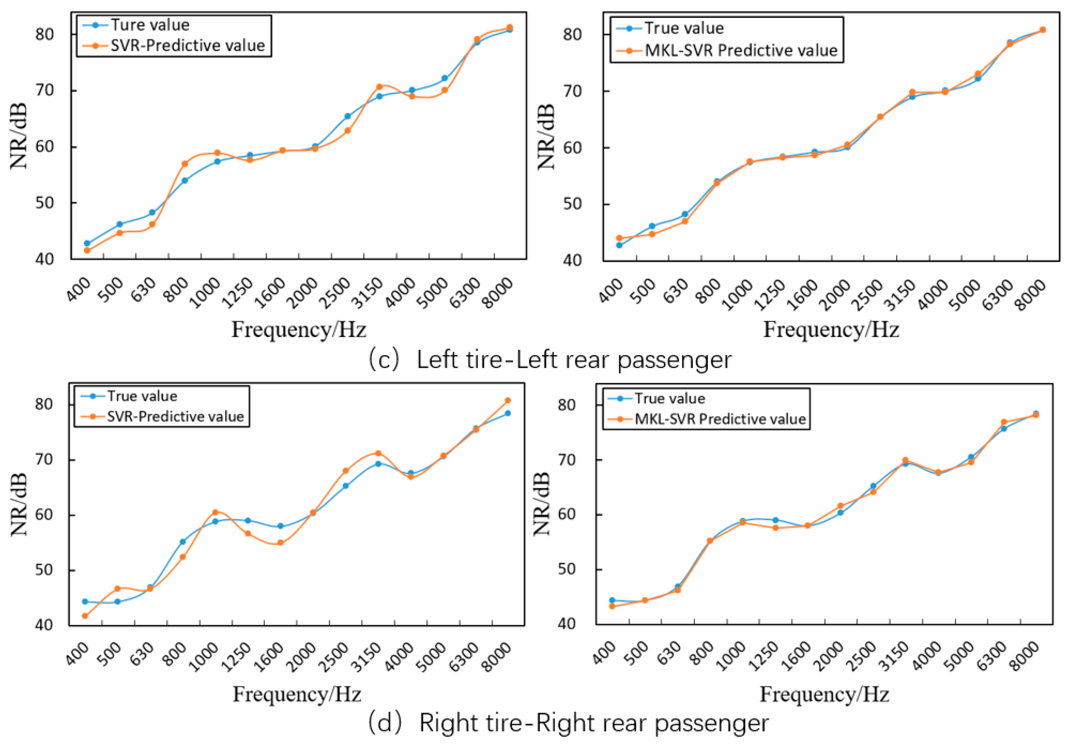
4.3. Prediction and Comparative Analysis of the Sound Insulation Performance of the MKL-SVR Model

Using the MKL-SVR model constructed in Section 4.2, the target prediction of the plate level, system level, and vehicle level was carried out from bottom to top for the sound insulation system of the vehicle body. Finally, the corresponding prediction results were obtained along the noise transmission path in the vehicle. The results of vehicle-level noise attenuation are shown in Figure 11. Among them, the ‘MKL-SVR predicted value‘ is the predicted result under the multi-core learning mode, and the data collected from the vehicle sound insulation performance test of the series ‘prototype’ is the ‘true value’. The accuracy of the model prediction results was tested. From Figure 11, it can be seen that for (a) the left front wheel—driver, (b) the right front wheel—co-driver, (c) the left rear wheel—left rear passenger, (d) the right rear wheel—right rear passenger, the left side of each vehicle path is the comparison chart between the single-core SVR and the true value, and the right side is the comparison chart between the MKL-SVR and the true value. It can be clearly concluded that the predicted values of the MKL-SVR model and the SVR model of the noise attenuation are consistent with the linear trend in the real value. On this basis, the prediction results of the SVR model in the MKL mode were compared with the prediction results of the single kernel SVR model. The prediction results of the MKL-SVR model not only have a higher degree of coincidence with the real value trend but also have better accuracy.

In order to discuss the results of the two models more clearly and accurately, the relative error analysis of the single-kernel SVR model and the MKL-SVR model was carried out, and the RMS value of the one-third octave sound insulation performance index was calculated. In this paper, the average and maximum values of the relative error of the data are used to analyze the error of the prediction results, as shown in Equations (18) and (19):

$${\epsilon }_{ave}=\frac{1}{n}{{\displaystyle \sum }}_{i=1}^n\frac{\widetilde{RM{S}_l}-\widehat{RM{S}_l}}{RM{S}_i}$$

(18)

$${\epsilon }_{max}=\max {{\displaystyle \sum }}_{i=1}^n\frac{\widetilde{RM{S}_l}-\widehat{RM{S}_l}}{RM{S}_i}$$

(19)

where $n$ is the number of samples in the test set, $\widetilde{RM{S}_l}$ is the RMS predicted value of the sound insulation performance of the ith test sample, and $\widehat{RM{S}_l}$ is the RMS true value of the sound insulation performance of the ith test sample.

Using the above formulas, the average and maximum relative errors of noise attenuation in the four paths of left front wheel—driver, right front wheel—co-driver, left rear wheel—left rear passenger, and right rear wheel—right rear passenger are obtained, respectively. The results are shown in

Table 4. Average value analysis of the relative error prediction of noise attenuation in the vehicle interior noise transfer path.

Noise Transfer Path	Single-Core Learning			MKL
	Gaussian Kernel	Polynomial Kernel	Sigmoid Kernel	MKL-SVR
left tire—driver	2.65%	2.73%	2.71%	1.17%
right tire—co driver	2.15%	2.92%	2.38%	0.84%
left tire—left rear passenger	2.73%	2.95%	2.81%	1.25%
right tire—right rear passenger	2.61%	2.69%	2.75%	1.40%

and

Table 5. Analysis of the maximum relative error of noise attenuation prediction in the vehicle interior noise transfer path.

Noise Transfer Path	Single-Core Learning			MKL
	Gaussian Kernel	Polynomial Kernel	Sigmoid Kernel	MKL-SVR
left tire—driver	2.49%	1.07%	2.65%	1.17%
right tire—co driver	1.84%	0.75%	2.15%	0.84%
left tire—left rear passenger	2.64%	1.18%	2.73%	1.25%
right tire—right rear passenger	2.54%	1.21%	2.61%	1.40%

. In the relative error analysis table, the kernel functions of the single-kernel SVR include the Gaussian kernel function, the polynomial kernel function, and the sigmoid kernel function. The prediction results of the single-kernel SVR model with three different kernel functions are analyzed and compared with the prediction results of the MKL-SVR model. The best effect of the single-kernel SVR model is the SVR model with the Gaussian kernel function, and the average relative error is 1.84%~2.64%. The average relative error of the MKL-SVR model is reduced to 0.75%~1.21%, which is lower than the average relative error of the three single-core SVR models. At the same time, the average relative error of the SVR model with the Gaussian kernel function is 2.15%~2.73%, and the maximum relative error in the MKL mode is reduced to less than 1.50%, which is less than the maximum relative error of the three single-kernel SVR models. This further shows that the stability of the MKL-SVR model is also improved to a certain extent.

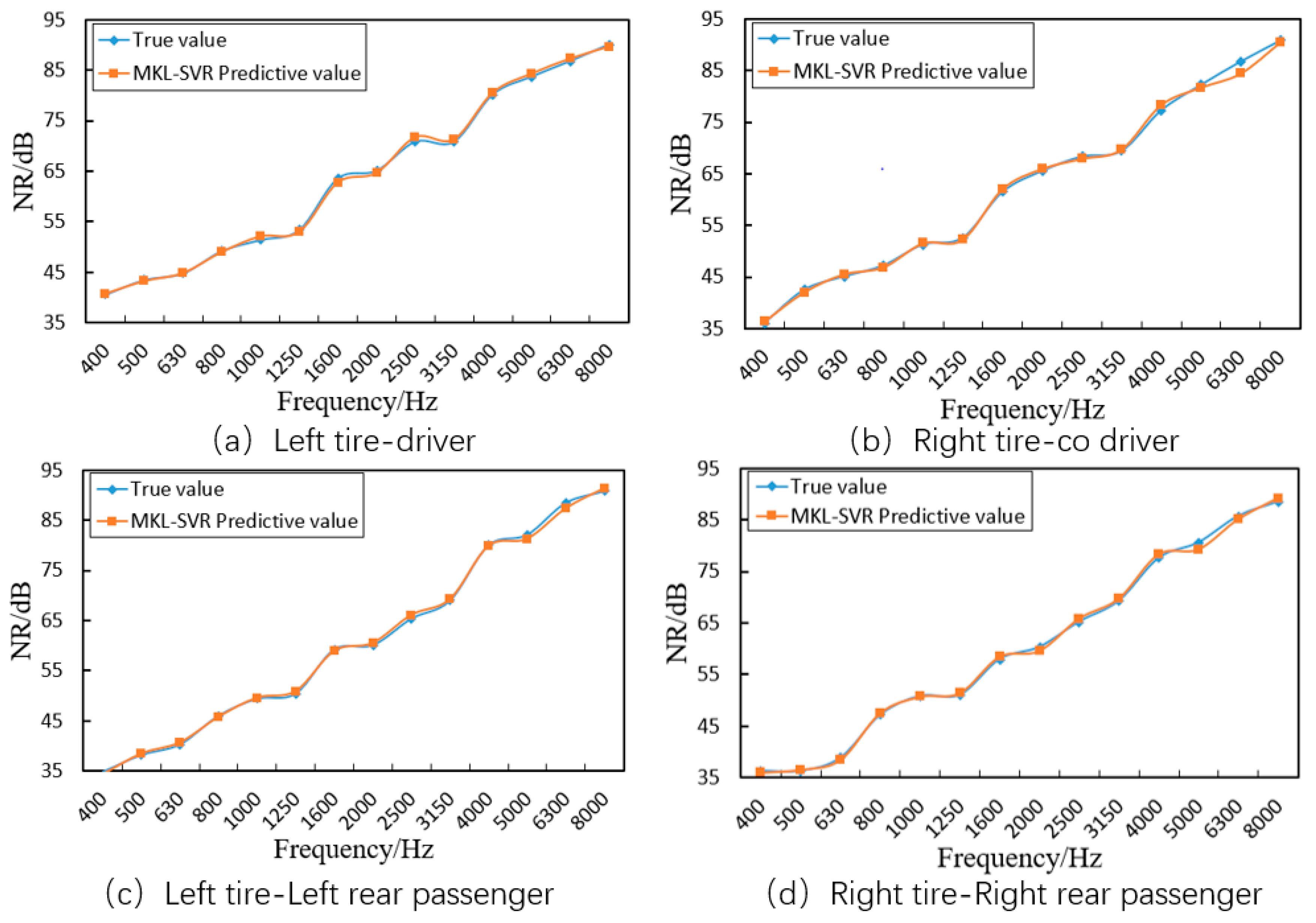
4.4. Sound Insulation Performance Verification of the MKL-SVR Model

The validation set data is completely independent of the parameter adjustment and training process of the previous model, which represents the generalization and universality of the prediction model in practical engineering application scenarios. The validation data set was imported into the well-trained MKL-SVR prediction model, and then the sound insulation performance of the acoustic package was predicted step by step, and the verification effect of the model was evaluated. The results of the MKL-SVR model using the validation set data for prediction are shown in Figure 12.

According to Figure 12, it can be seen that the MKL-SVR prediction model established in this paper has a significant effect, and the true value of the verification set is highly coincident with the trend in the model prediction value. It can be seen from

Table 6. MKL-SVR model validation set error analysis.

Path	Average Relative Error	Maximum Relative Error
left tire—driver	1.22%	1.30%
right tire—co driver	1.09%	1.37%
left tire—left rear passenger	0.86%	1.06%
right tire—right rear passenger	1.09%	0.96%

that the average relative errors of the prediction results of the four path models are 1.22%, 1.09%, 0.86%, and 1.09%, respectively, and the maximum relative errors are 1.30%, 1.37%, 1.06%, and 0.96%, respectively. The relative error of the MKL-SVR model prediction results based on the validation set data is less than 1.5%, indicating that the model not only has high prediction accuracy but also has robustness.

5. Conclusions

(1)

A decomposition framework for predicting the sound insulation performance of the body system is established based on the analysis of the noise transmission path. This framework comprises the ‘vehicle level’, ‘component level’, and ‘panel level’, encompassing the dominant propagation mechanism of air sound in a vehicle, such as ‘tire noise’. Quantitative indicators of sound absorption and insulation performance for each unit at different levels are determined and correlated from top to bottom. The sound insulation performance of the body system is predicted step by step from bottom to top, aiming to reveal the quantitative relationship between related unit indicators within the hierarchical system.

(2)

The SVR method is introduced based on the decomposition architecture to elucidate the quantitative relationship between related unit indexes within the hierarchical system. This step is taken to overcome inherent weaknesses in conventional CAE processes, including challenging physical mechanisms, cumbersome basic data preparation, and modeling operations. Consequently, a machine learning model for predicting the sound insulation performance of the body system is established, laying a foundation for ensuring prediction accuracy and efficiency. In specific processing, sound absorption and insulation performance indicators at each level are presented in the form of a ‘frequency characteristic curve’. Given that the single-kernel SVR model necessitates characterizing the mapping relationship between corresponding frequency data of related element indicators, a ‘step-by-step and frequency-by-frequency analysis’ data processing format is used. Subsequently, the MKL method is used to introduce the weighted kernel, enhancing the processing effectiveness of the single-kernel SVR model.

(3)

The proposed method underwent application and testing on a specific vehicle model, involving core aspects such as sample data structure, data sample expansion in machine learning, SVR prediction model configuration, and model training, testing, and verification. The results demonstrate excellent agreement between predicted and real values. In comparison with the single-kernel learning mode, the MKL mode significantly improves prediction accuracy and stability. The evident advantages in prediction accuracy indicate a promising prospect for the widespread adoption and application of the proposed method.

(4)

The MKL-SVR method has high accuracy in solving complex problems of high-dimensional and heterogeneous data, and the effectiveness of this method is widely recognized in various fields. However, this method also lacks a theoretical basis for the selection and combination of basic kernels. Using a repeated learning SVR model to determine the weight relationship between multiple kernel functions will increase the workload, and the learning efficiency of the MKL learning method for large-scale data sets will be low. The existence of these problems makes the research of multi-kernel learning support vector learning still worthy of in-depth discussion by researchers.

References

1. Pietrusiak, D.; Wróbel, J.; Czechowski, M.; Fiebig, W. Numerical and Experimental NVH Testing of Vehicle Components—From Simple Part to Complex Assembly. MATEC Web Conf. 2022, 357, 12. [Google Scholar] [CrossRef]
2. Lee, J.; Shin, J.; Kwon, O.C.; Kim, G. A study on configuration of acoustic package for towed array sonar using design of experiments. J. Acoust. Soc. Korea 2019, 2, 200–206. [Google Scholar] [CrossRef]
3. Zhang, Y.; Li, L.; Zhu, Q. Structure-borne Noise Differences of Metro Vehicle Running on Different Tracks. KSCE J. Civ. Eng. 2023, 27, 3861–3871. [Google Scholar] [CrossRef]
4. Mao, Z.; Lin, Y.S. Application of sound package material in noise reduction of motor. Vibroengineering Procedia 2021, 36, 27702–27718. [Google Scholar] [CrossRef]
5. Oettle, N.; Sims, W.D. Automotive aeroacoustics: An overview. Proc. Inst. Mech. Eng. Part D J. Automob. Eng. 2017, 231, 1177–1189. [Google Scholar] [CrossRef]
6. Neubauer, R.O. Advanced Rating Method of Airborne Sound Insulation. Appl. Sci. 2016, 6, 322. [Google Scholar] [CrossRef]
7. Fernández de las Heras, M.J.; Chimeno Manguán, M.; Roibás Millán, E.; Simón Hidalgo, F. Determination of SEA loss factors by Monte Carlo Filtering. J. Sound Vib. 2020, 479. [Google Scholar] [CrossRef]
8. Sohrabi, S.; Segura Torres, A.; Cierco Molins, E.; Perazzolo, A.; Bizzarro, G.; Rodríguez Sorribes, P.V. A Comparative Study of a Hybrid Experimental–Statistical Energy Analysis Model with Advanced Transfer Path Analysis for Analyzing Interior Noise of a Tiltrotor Aircraft. Appl. Sci. 2023, 13, 12128. [Google Scholar] [CrossRef]
9. Zhang, J.; Xiao, X.; Sheng, X.; Yao, D.; Wang, R. An acoustic design procedure for controlling interior noise of high-speed trains. Appl. Acoust. 2020, 168, 107419. [Google Scholar] [CrossRef]
10. Chen, S.; Zhou, Z.; Zhang, J. Multi-objective optimisation of automobile sound package with non-smooth surface based on grey theory and particle swarm optimisation. Int. J. Veh. Des. 2022, 88, 238–259. [Google Scholar] [CrossRef]
11. Kamal, K.; Luca, A.; Noureddine, A. Comments on the validity of transfer matrix based models for the prediction of the effect of curved sound packages. J. Sound Vib. 2020, 465, 114990. [Google Scholar] [CrossRef]
12. Jin, J.; Zhu, C.; Wu, R.; Liu, Y.; Li, M. Comparative noise reduction effect of sound barrier based on statistical energy analysis. J. Comput. Methods Sci. Eng. 2021, 21, 737–745. [Google Scholar] [CrossRef]
13. Su, J.; Zheng, L.; Deng, Z.; Jiang, Y. Research Progress on High-Intermediate Frequency Extension Methods of SEA. Shock. Vib. 2019, 2019, 4192437. [Google Scholar] [CrossRef]
14. Hugues, P.; Elsa, P.; Annie, R. An acoustic trade-off chart for the design of multilayer acoustic packages. Appl. Acoust. 2019, 148, 9–18. [Google Scholar] [CrossRef]
15. Wang, F.; Chen, Z.; Wu, C.; Yang, Y. Prediction on sound insulation properties of ultrafine glass wool mats with artificial neural networks. Appl. Acoust. 2019, 146, 164–171. [Google Scholar] [CrossRef]
16. Satyanarayana, G.S.R.; Deshmukh, P.; Das, S. Vehicle detection and classification with spatio-temporal information obtained from CNN. Displays 2022, 75, 102294. [Google Scholar] [CrossRef]
17. Ju, H.J.; Sung, S.Y.; Yeon, J.K. Estimation of sound absorption coefficient of layered fibrous material using artificial neural networks. Appl. Acoust. 2020, 169, 107476. [Google Scholar] [CrossRef]
18. Lee, H.; Kim, D.; Gu, J. Prediction of Food Factory Energy Consumption Using MLP and SVR Algorithms. Energies 2023, 16, 1550. [Google Scholar] [CrossRef]
19. Huang, H.; Huang, X.; Ding, W.; Yang, M.; Yu, X.; Pang, J. Vehicle vibro-acoustical comfort optimization using a multi-objective interval analysis method. Expert Syst. Appl. 2023, 213, 119001. [Google Scholar] [CrossRef]
20. Choi, D.; Yim, J.; Baek, M.; Lee, S. Machine learning-based vehicle trajectory prediction using v2v communications and on-board sensors. Electronics 2021, 10, 420. [Google Scholar] [CrossRef]
21. Huang, H.; Lim, T.C.; Wu, J.; Ding, W.; Pang, J. Multitarget prediction and optimization of pure electric vehicle tire/road airborne noise sound quality based on a knowledge-and data-driven method. Mech. Syst. Signal Process. 2023, 197, 15. [Google Scholar] [CrossRef]
22. Pau, D.; Ben, Y.W.; Aymone, F.M.; Licciardo, G.D.; Vitolo, P.T. Tiny Machine Learning Zoo for Long-Term Compensation of Pressure Sensor Drifts. Electronics 2023, 12, 4819. [Google Scholar] [CrossRef]
23. Hu, S.; Meng, Y.; Zhang, Y. Prediction Method for Sugarcane Syrup Brix Based on Improved Support Vector Regression. Electronics 2023, 12, 1535. [Google Scholar] [CrossRef]
24. Xian, H.; Che, J. Unified whale optimization algorithm based multi-kernel SVR ensemble learning for wind speed forecasting. Appl. Soft Comput. J. 2022, 130, 109690. [Google Scholar] [CrossRef]
25. Xiao, J.; Wei, C.; Liu, Y. Speed estimation of traffic flow using multiple kernel support vector regression. Phys. A Stat. Mech. Its Appl. 2018, 509, 989–997. [Google Scholar] [CrossRef]
26. Huang, H.; Huang, X.; Ding, W.; Zhang, S.; Pang, J. Optimization of electric vehicle sound package based on LSTM with an adaptive learning rate forest and multiple-level multiple-object method. Mech. Syst. Signal Process. 2023, 187, 109932. [Google Scholar] [CrossRef]
27. Huang, H.; Huang, X.; Ding, W.; Yang, M.; Fan, D.; Pang, J. Uncertainty optimization of pure electric vehicle interior tire/road noise comfort based on data-driven. Mech. Syst. Signal Process. 2022, 165, 15. [Google Scholar] [CrossRef]
28. Huang, X.; Huang, H.; Wu, J.; Yang, M.; Ding, W. Sound quality prediction and improving of vehicle interior noise based on deep convolutional neural networks. Expert Syst. Appl. 2020, 160, 1. [Google Scholar] [CrossRef]
29. Wu, R.; Liu, B.; Fu, J.; Xu, M.; Fu, P.; Li, J. Research and Implementation of ε-SVR Training Method Based on FPGA. Electronics 2019, 8, 919. [Google Scholar] [CrossRef]
30. Sheng, B.; Li, J.; Xiao, F.; Yang, W. Multilayer deep features with multiple kernel learning for action recognition. Neurocomputing 2020, 399, 65–74. [Google Scholar] [CrossRef]
31. Chen, B.; Zheng, K.D.; Wang, K.H. Research on multi-kernel support vector regression method. Intell. Comput. Appl. 2019, 1, 188–191. Available online: https://www.cqvip.com/qk/94259a/20191/7001054339.html (accessed on 30 January 2019).
32. Wang, X.; Zheng, Q.; Zheng, K.; Wu, T. User Authentication Method Based on MKL for Keystroke and Mouse Behavioral Feature Fusion. Secur. Commun. Netw. 2020, 2020, 9282380. [Google Scholar] [CrossRef]
33. Sheng, H.; Wang, S.T. Style regularized least squares support vector machine based on multi-kernel learning. Comput. Sci. Explor. 2020, 9, 1532–1544. Available online: https://kns.cnki.net/kcms2/article/abstract?v=GARc9QQj0GWx0EZ7eNx0g-pNDGz75x9QFofDaHm-bdESuPeD0fa3t0nW3kzEjSB254Ui_CQHQggcLMGn7lyP77wYjXp09D-ui-hivxLkSk8waOiWichVqH2iOp9CaU9kQOEGW0LKAR40cDSVfa0uFg==&uniplatform=NZKPT&language=CHS (accessed on 1 September 2019).
34. Sedigheh, M.; Shahryar, R.; Mohammad, E.S. Multilevel framework for large-scale global optimization. Soft Comput. 2017, 21, 4111–4140. [Google Scholar] [CrossRef]
35. Wijegunawardana, I.D.; De Mel, W.R. Biomimetic designs for automobile engineering: A review. Int. J. Automot. Mech. Eng. 2021, 18, 9029–9041. [Google Scholar] [CrossRef]
36. Salmani, H.; Khalkhali, A.; Mohsenifar, A. A practical procedure for vehicle sound package design using statistical energy analysis. Proc. Inst. Mech. Eng. Part D J. Automob. Eng. 2023, 237, 3054–3069. [Google Scholar] [CrossRef]
37. Huang, H.; Wu, J.H.; Lim, T.C.; Yang, M.; Ding, W. Pure electric vehicle nonstationary interior sound quality prediction based on deep CNNs with an adaptable learning rate tree. Mech. Syst. Signal Process. 2021, 148, 107170. [Google Scholar] [CrossRef]
38. Basani, S.; Murthy, P.S.S.; Eswaraiah, K. Hierarchical parallel processing for design optimization—A case study. Mater. Today Proc. 2018, 2, 5117–5123. [Google Scholar] [CrossRef]
39. Li, H.; Zheng, X.; Dai, W.; Qiu, Y. Prediction of Ride Comfort of High-Speed Trains Based on Train Seat–Human Body Coupled Dynamics Model. Appl. Sci. 2022, 12, 12900. [Google Scholar] [CrossRef]
40. GB/Z 27764-2011; Measurement of Sound Transmission Loss in Acoustic Impedance Tube. National Acoustic Standardization Technical Committee, Standards Press of China: Beijing, China, 2011.
41. ISO 15186-1-2003; Acoustics Measurement of Sound Insulation in Buildings and of Building Elements Using Sound Intensity. International Organization for Standardization: Geneva, Switzerland, 2003.
42. Arturas, K.; Vidas, R. Analysis of Training Data Augmentation for Diabetic Foot Ulcer Semantic Segmentation. Electronics 2023, 22, 4624. [Google Scholar] [CrossRef]
43. Del Pizzo, L.G.; Bianco, F.; Moro, A.; Schiaffino, G.; Licitra, G. Relationship between tyre cavity noise and road surface characteristics on low-noise pavements. Transp. Res. Part D Transp. Environ. 2021, 98, 102971. [Google Scholar] [CrossRef]
44. Rao, D.; Zhang, D.; Lu, H.; Yang, Y.; Qiu, Y.; Ding, M.; Yu, X. Deep learning combined with Balance Mixup for the detection of pine wilt disease using multispectral imagery. Comput. Electron. Agric. 2023, 208, 107778. [Google Scholar] [CrossRef]
45. Wang, Y.; Ji, Y.; Xiao, H. A data augmentation method for fully automatic brain tumor segmentation. Comput. Biol. Med. 2022, 149, 106039. [Google Scholar] [CrossRef] [PubMed]
46. Hongyu, G. Nonlinear Mixup: Out-Of-Manifold Data Augmentation for Text Classification. Proc. AAAI Conf. Artif. Intell. 2020, 34, 4044–4051. [Google Scholar] [CrossRef]
Figure 1. SVR diagram. (○ is a sample falling outside the interval band, is a sample falling inside the interval band, the red thick dotted line is a linear function, and the area formed between the two red virtual and real lines is called the ‘interval band’).
Electronics 13 00538 g001
Figure 2. MKL-SVR model diagram.
Electronics 13 00538 g002
Figure 3. Decomposition architecture of the sound insulation performance prediction of the vehicle body system.
Electronics 13 00538 g003
Figure 4. Hierarchical decomposition of the sound insulation performance of the body system.
Electronics 13 00538 g004
Figure 5. Sound absorption and insulation principal diagram.
Electronics 13 00538 g005
Figure 6. Vehicle noise attenuation test diagram.
Electronics 13 00538 g006
Figure 7. Some experimental data on sound insulation performance.
Electronics 13 00538 g007
Figure 8. Sound absorption performance data of plates and components.
Electronics 13 00538 g008
Figure 9. Comparison of data enhanced samples and original samples. (a) The STL of front wall sheet metal. (b) The STL of inter front wall pad. (c) The STL of outer front wall pad. (d) The STL of front wall wind shield. (e) The STL of front wall.
Electronics 13 00538 g009aElectronics 13 00538 g009b
Figure 10. Training and testing of the prediction model.
Electronics 13 00538 g010
Figure 11. Prediction results of noise attenuation in the vehicle interior noise transmission path.
Electronics 13 00538 g011aElectronics 13 00538 g011b
Figure 12. Verification set noise attenuation prediction results.
Electronics 13 00538 g012