
Intelligent Design Optimization for Traction and Steering Motors of an Autonomous Electric Shuttle under Driving Scenarios


Abstract
:1. Introduction
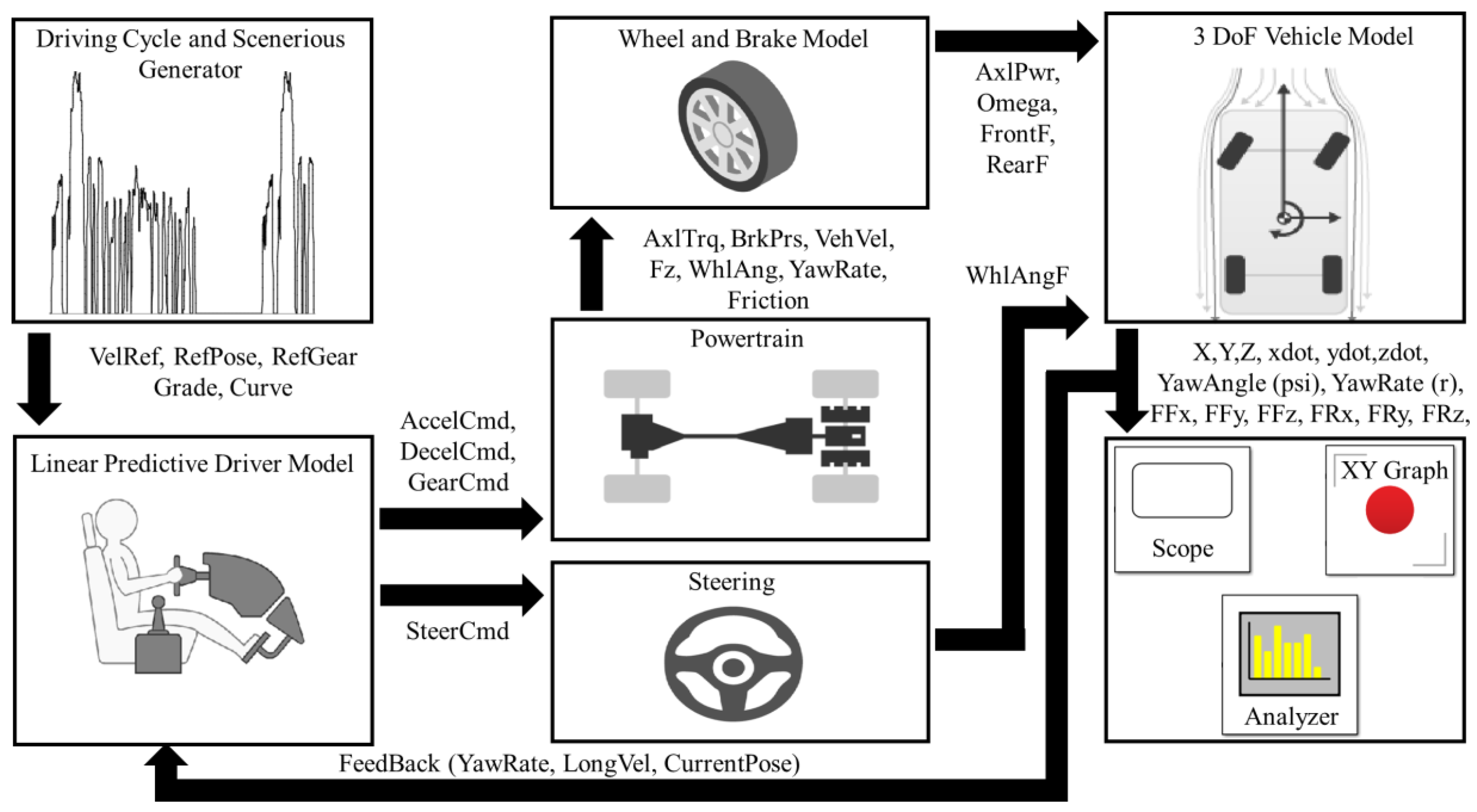
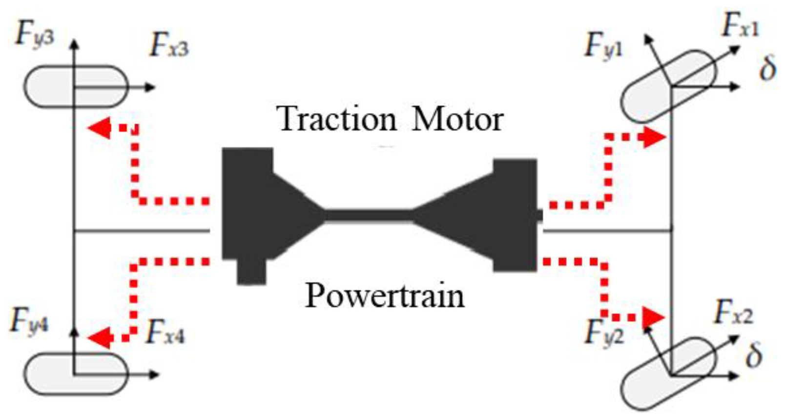
1.1. Vehicle Model
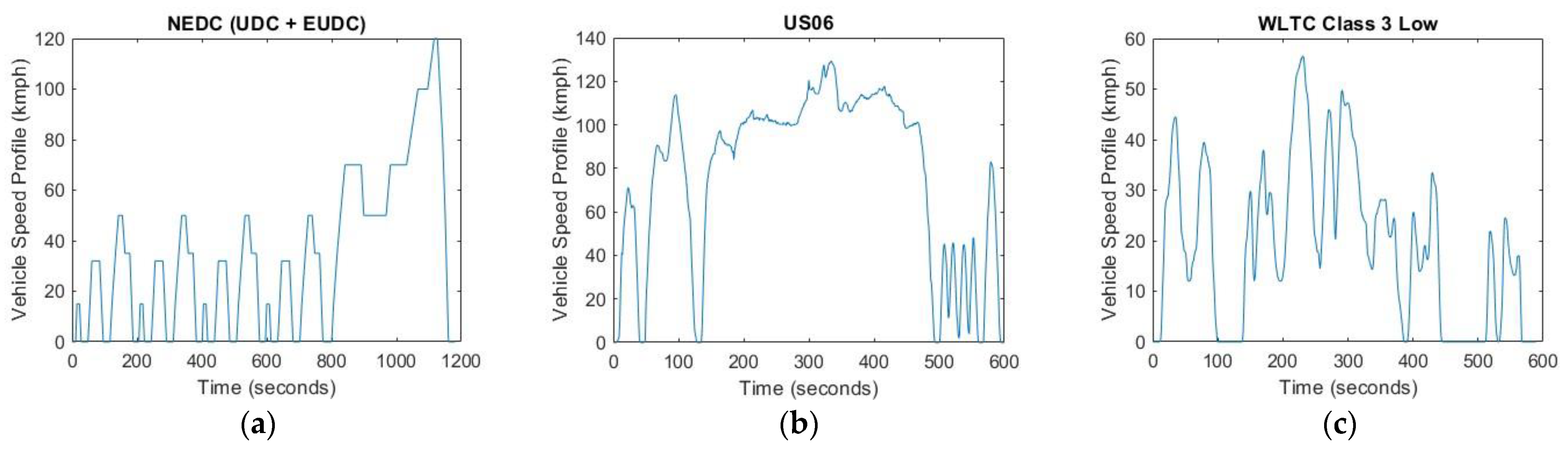
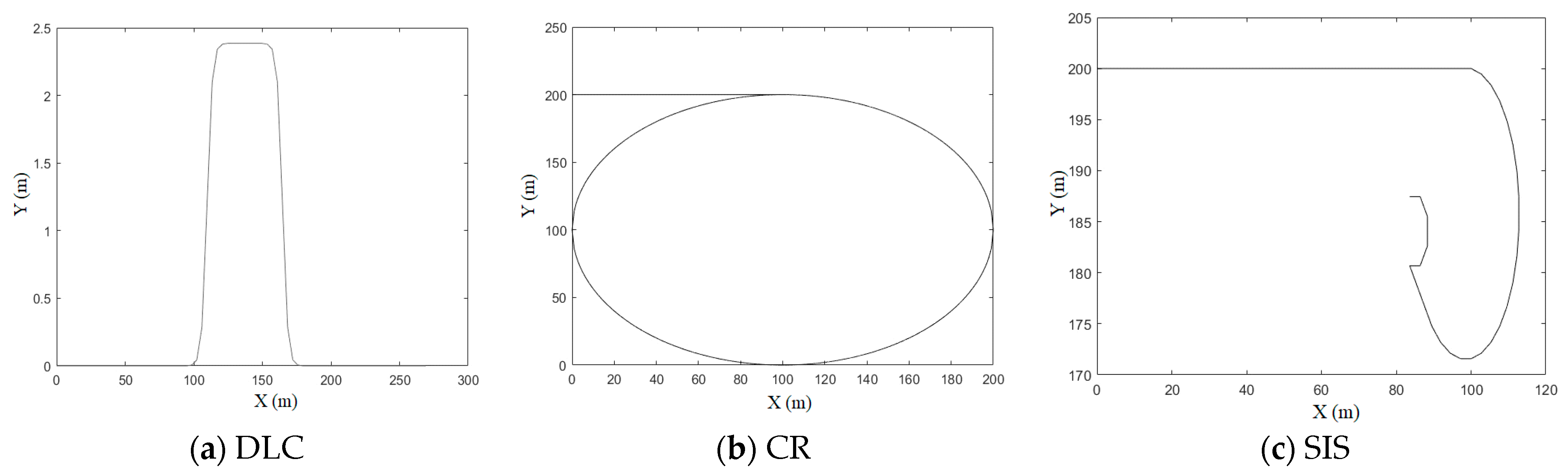
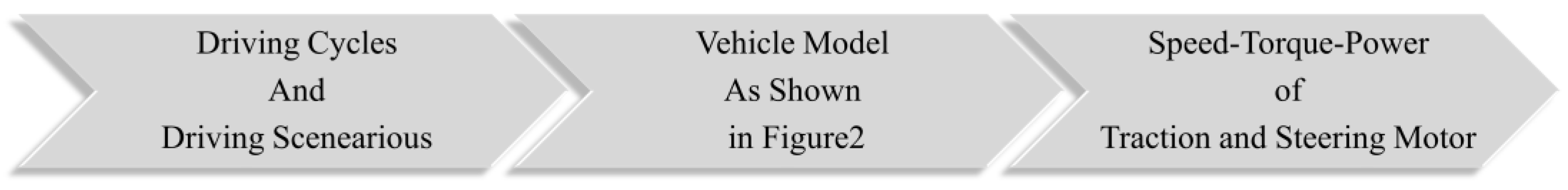
1.2. Driving Cycle and Scenarios
2. Materials and Methods
2.1. Objective Function
2.2. Optimization Algorithm
3. Results and Discussion
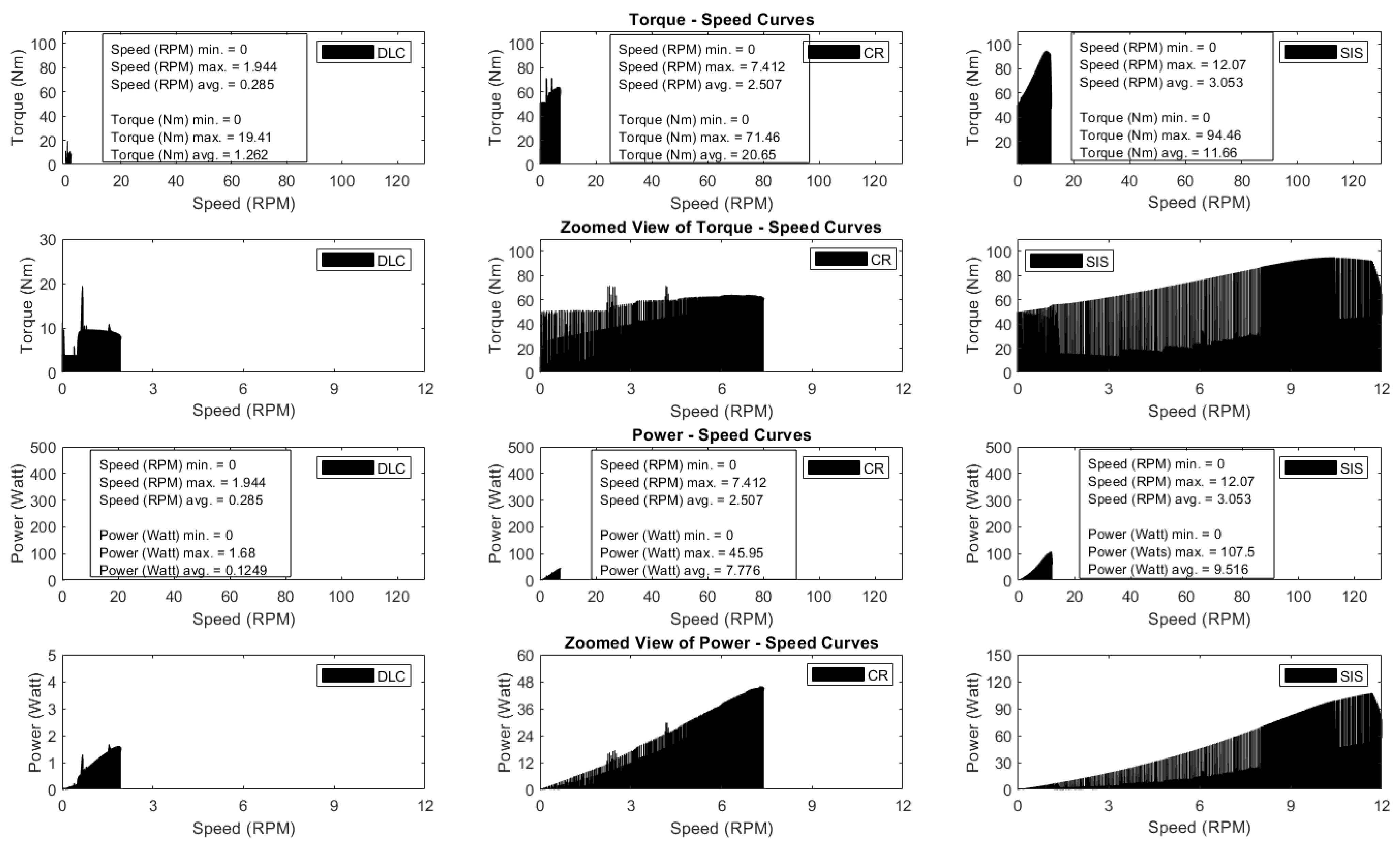
3.1. The Determination of Minimum Performance Requirements for Traction and Steering Motors
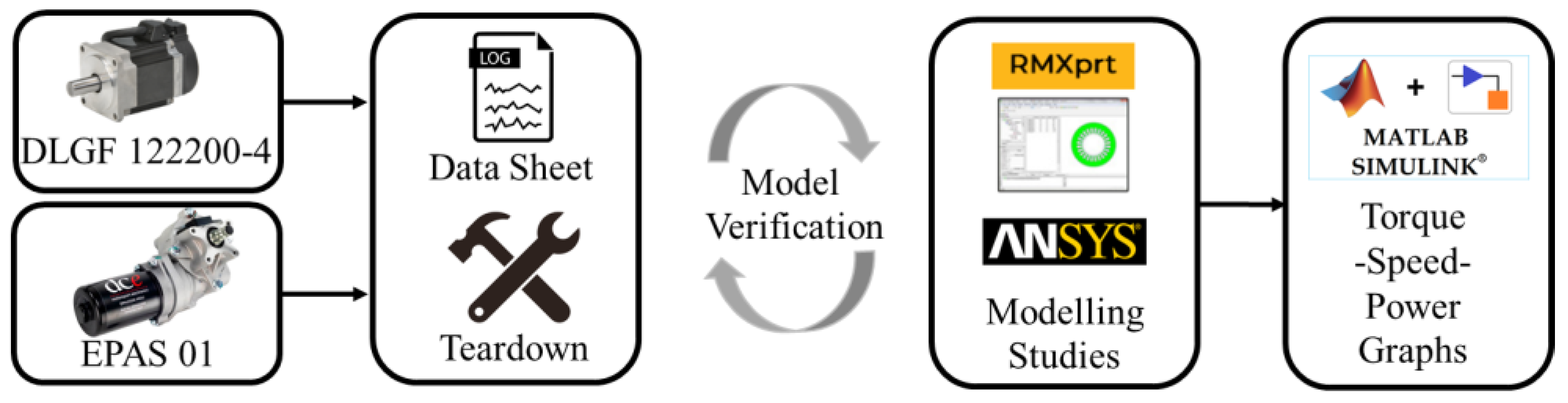
3.2. Modeling of Traction and Steering Motors
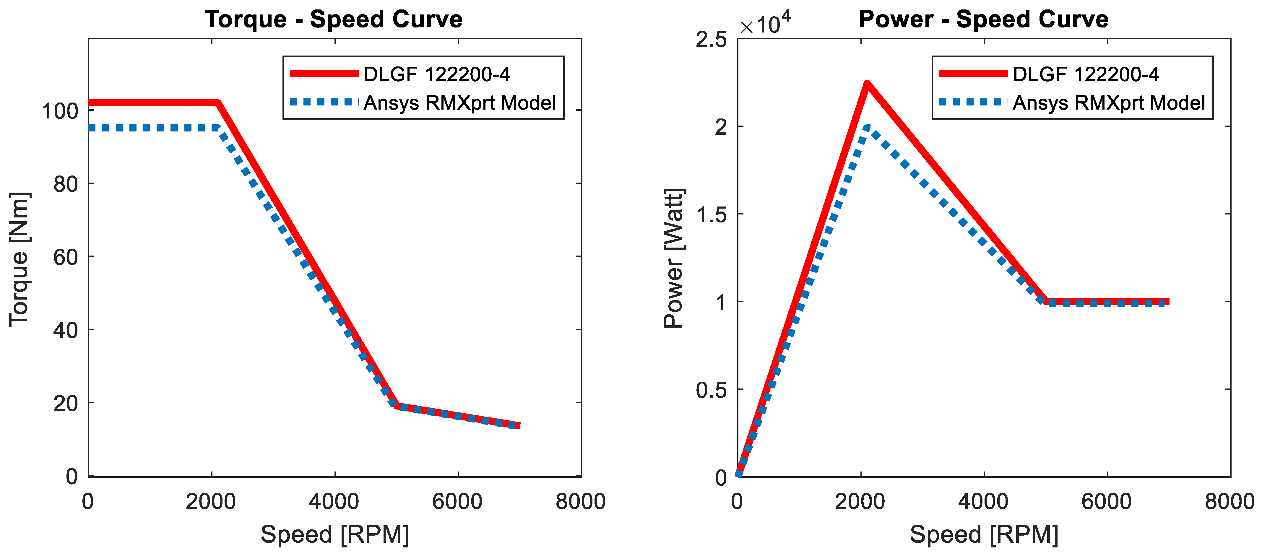
3.2.1. Modeling Studies for Traction Motor
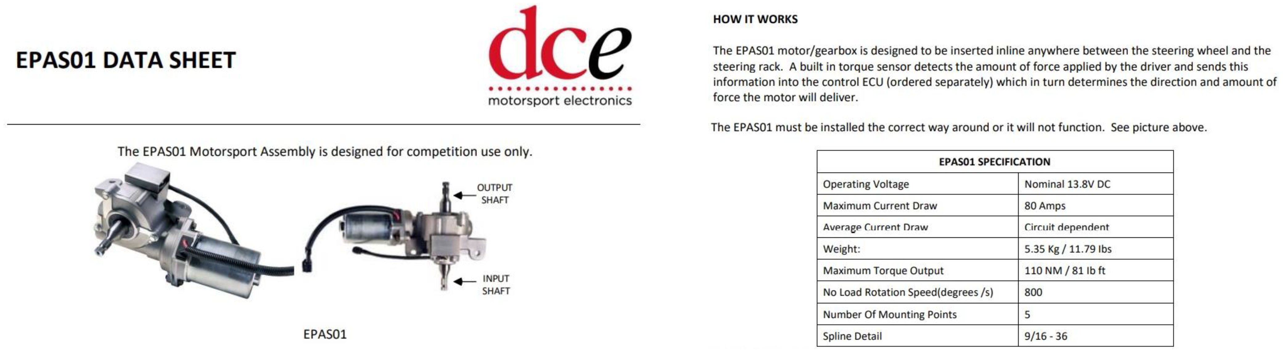
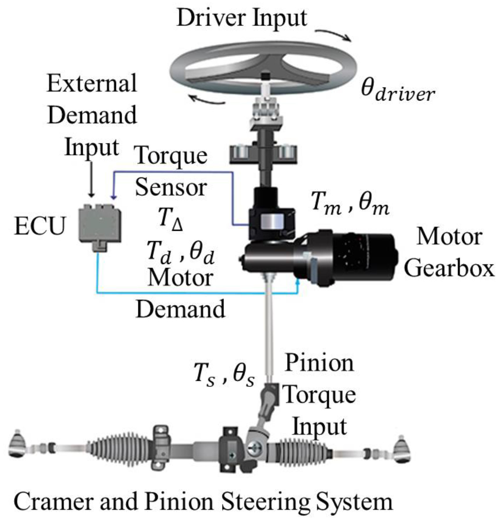
3.2.2. Modeling Studies for Steering Motor
3.3. Comparison of Minimum Performance Requirements for Traction and Steering Motors
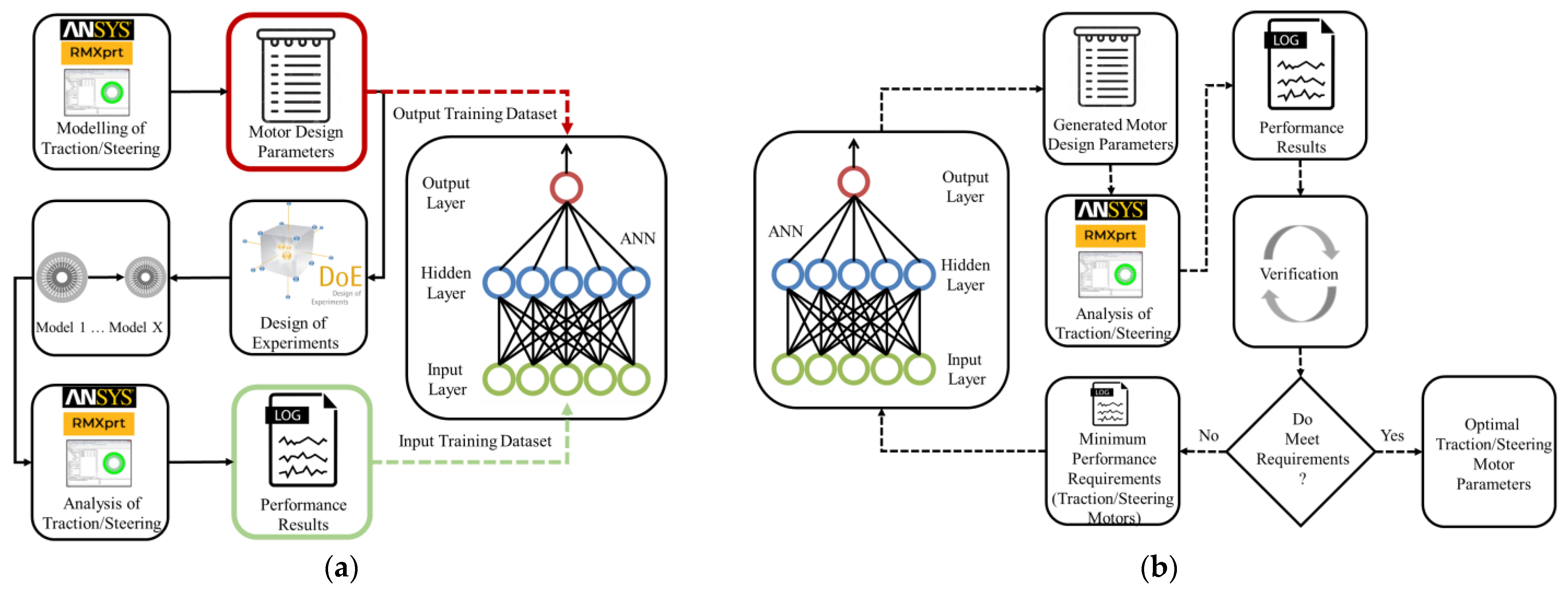
3.4. Creating Training Dataset and Training ANN for Optimization
3.4.1. Experimental Design and Preparation of ANN Training Dataset for Traction Motor
3.4.2. Experimental Design and Preparation of ANN Training Dataset for Steering Motor
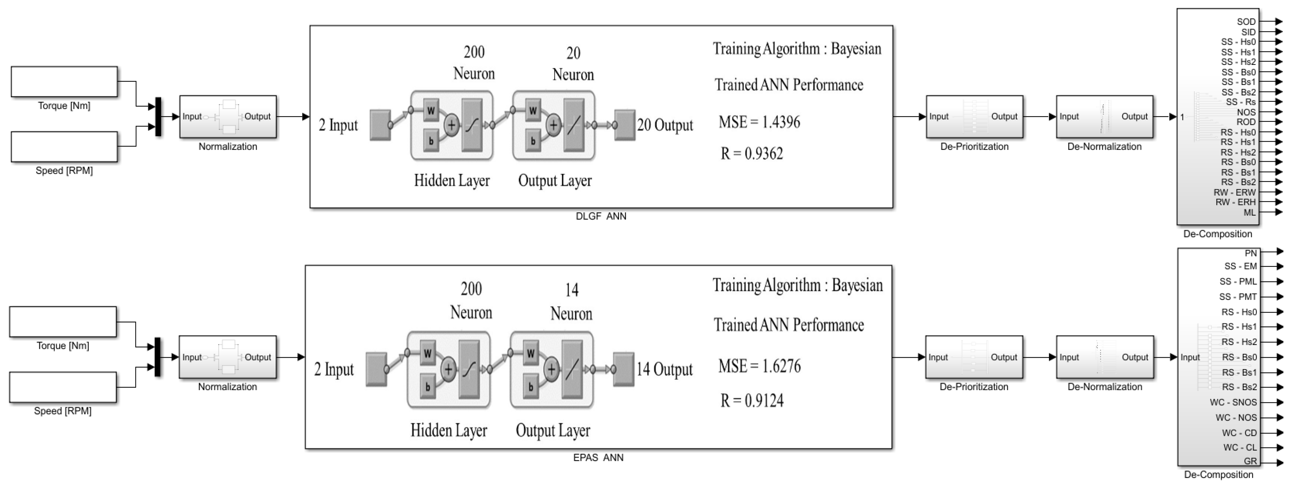
3.4.3. ANN Training of Traction and Steering Motors for Design Parameters’ Estimation
3.5. Generation of Motor Design Parameters and Motor Variations with ANN
3.6. Analysis of Motor Design Parameters Generated by ANN
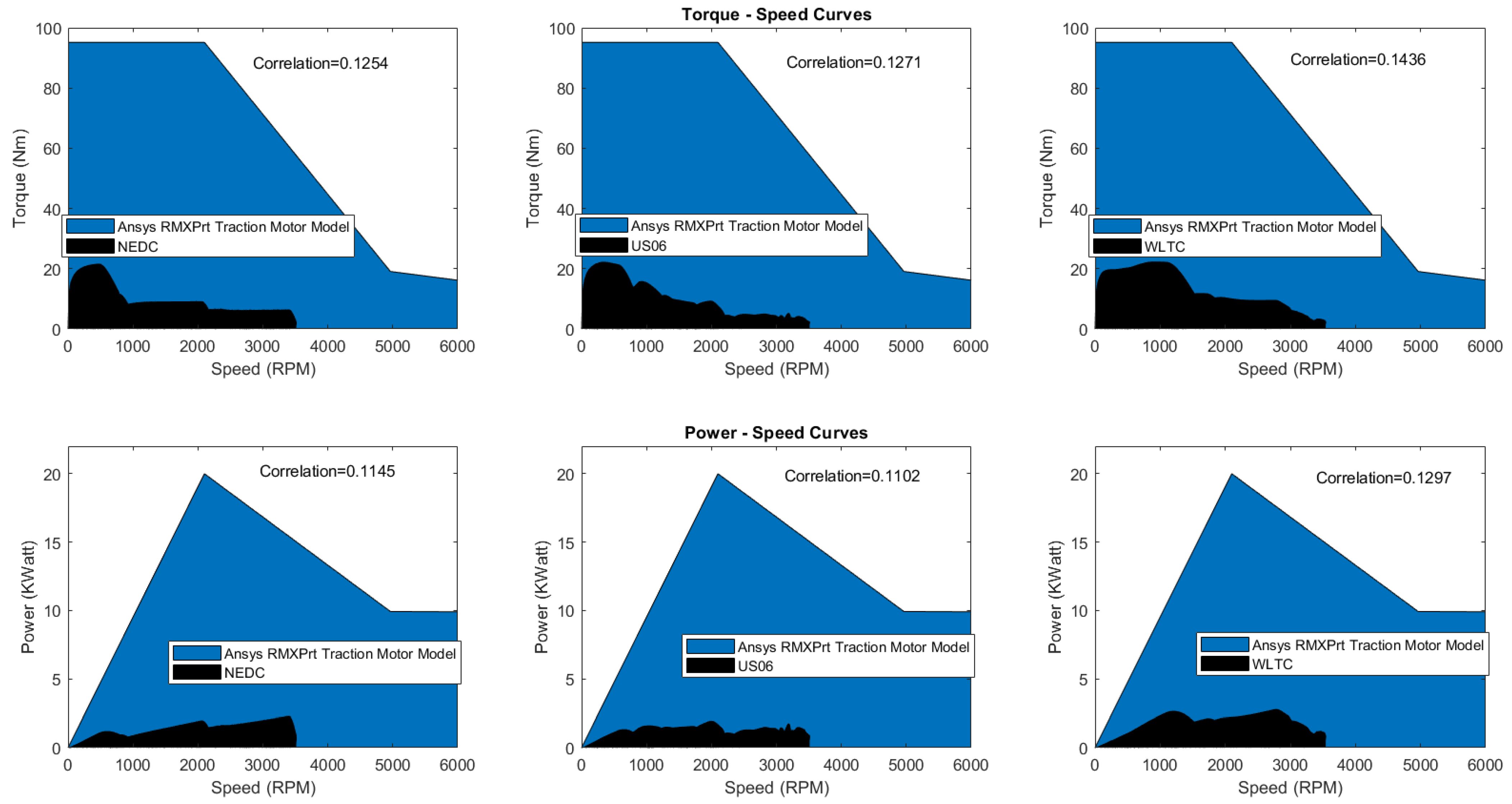
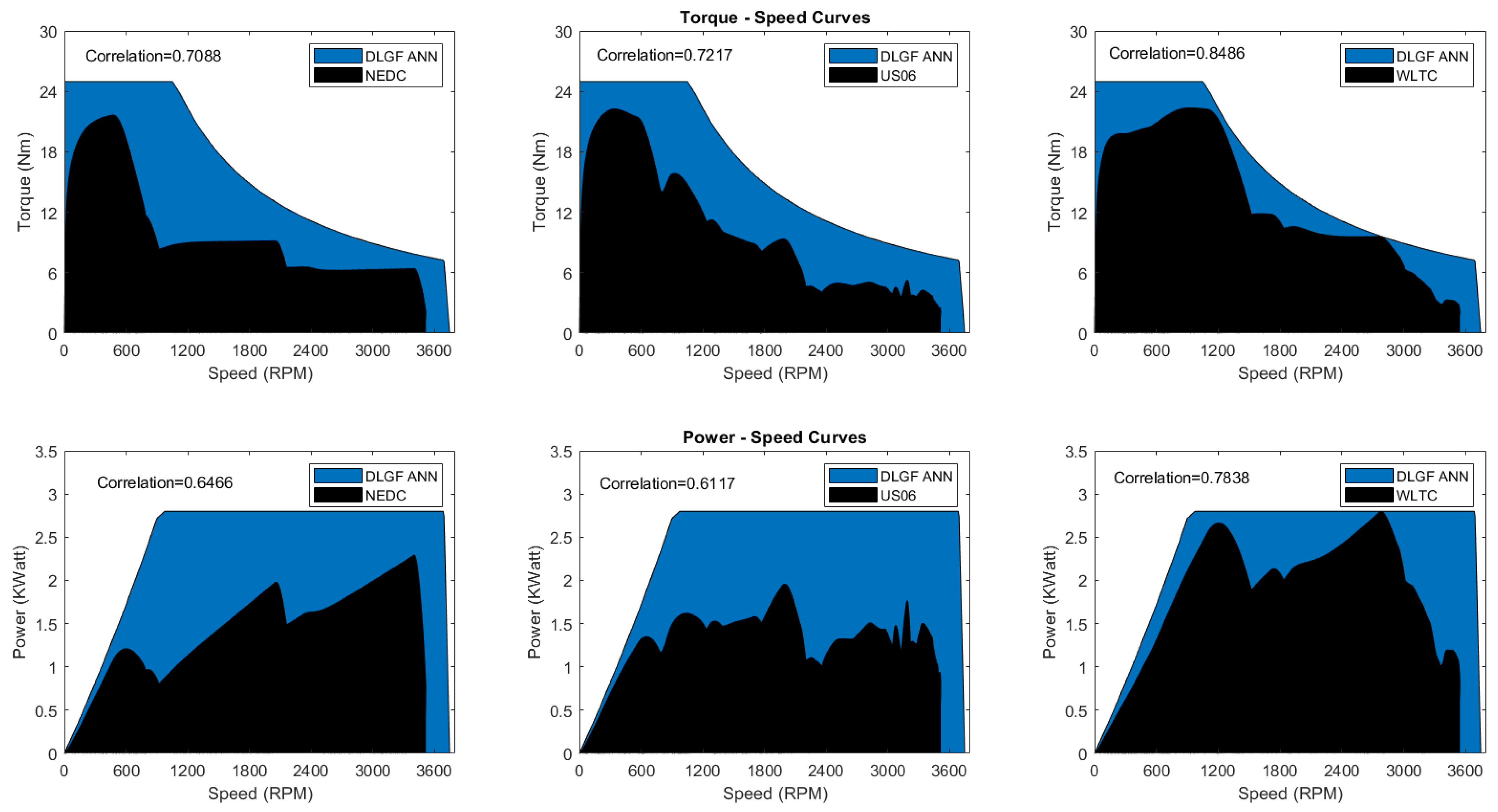
3.7. Comparison of Traction Motor Torque–Speed Curves Obtained under Driving Cycles and Torque–Speed Curves Generated by ANN
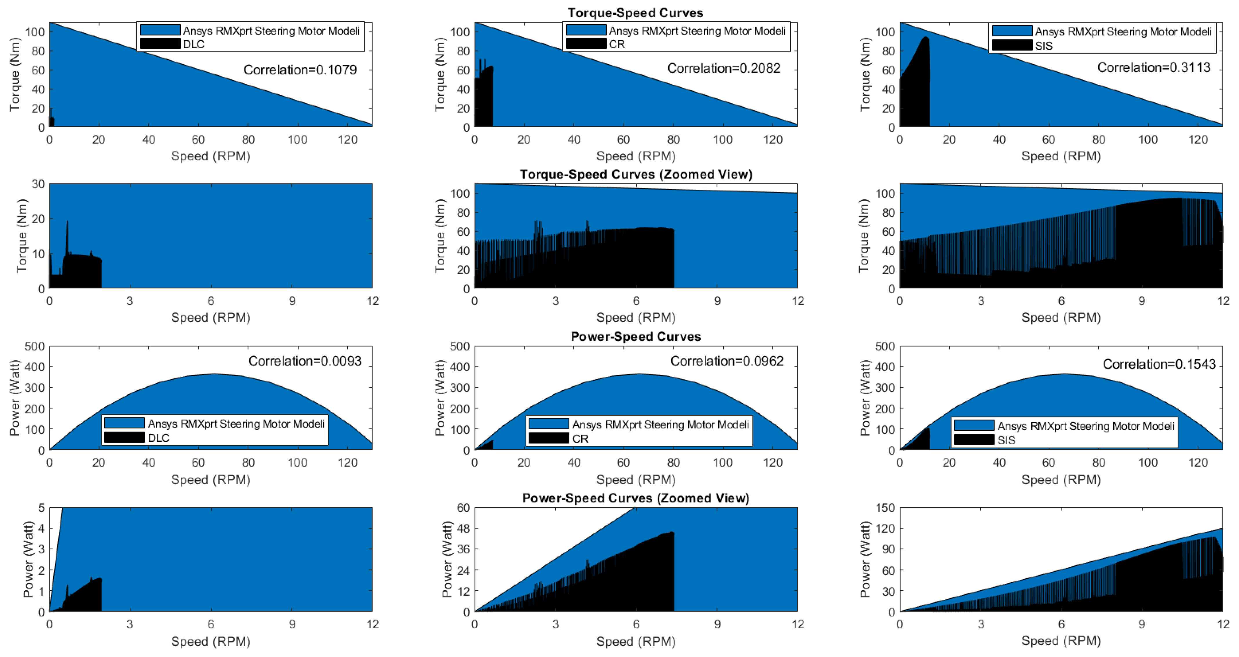
3.8. Comparison of Steering Motor Torque–Speed Curves Obtained under Driving Scenarios and Torque–Speed Curves Generated by ANN
3.9. Discussion of Analysis Results for Traction and Steering Motors Generated by ANN
4. Conclusions
- It has been observed that drive cycles and driving scenarios can be used not only to measure the dynamic performance and fuel consumption of existing vehicles, but also to calculate the required engine performance requirements.
- It has been observed that the minimum performance requirements determined by driving cycles and scenarios can determine the optimization criteria for an over-qualified motor selected by “over-designing”.
- It has been observed that the ANN is an effective method for estimating design parameters. Further, engine design parameters can be determined successfully in accordance with the performance requirements.
- It has been observed that using the ANN and DoE together not only shortens the training time, but also provides a better performance by training on meaningful data and qualifying the weight values in the ANN with DoE.
Author Contributions
Funding
Data Availability Statement
Acknowledgments
Conflicts of Interest
Appendix A

Appendix B
References
- Shen, H.; Wang, Z.; Zhou, X.; Lamantia, M.; Yang, K.; Chen, P.; Wang, J. Electric Vehicle Velocity and Energy Consumption Predictions Using Transformer and Markov-Chain Monte Carlo. IEEE Trans. Transp. Electrif. 2022, 8, 3836–3847. [Google Scholar] [CrossRef]
- Hu, D.; Huang, C.; Yin, G.; Li, Y.; Huang, Y.; Huang, H.; Wu, J.; Li, W.; Xie, H. A transfer-based reinforcement learning collaborative energy management strategy for extended-range electric buses with cabin temperature comfort consideration. Energy 2024, 290, 130097. [Google Scholar] [CrossRef]
- Shi, J.; Xu, B.; Zhou, X.; Hou, J. A cloud-based energy management strategy for hybrid electric city bus considering real-time passenger load prediction. J. Energy Storage 2022, 45, 103749. [Google Scholar] [CrossRef]
- Ehsani, M.; Gao, Y.; Emadi, A. Modern Electric, Hybrid Electric, and Fuel Cell Vehicles—Fundamentals, Theory, and Design, 2nd ed.; CRC Press; Taylor and Francis Group, LLC: Boca Raton, FL, USA, 2010. [Google Scholar] [CrossRef]
- Christensen, T.; Sørensen, N.B.; Bøg, B. Energy Efficient Control of an Induction Machine for an Electric Vehicle. Master Thesis, Aalborg University, Study Board of Industry and Global Business Development, Aalborg East, Denmark, 2012. [Google Scholar] [CrossRef]
- Diao, K.; Sun, X.; Lei, G.; Bramerdorfer, G.; Guo, Y.; Zhu, J. System-level Robust Design Optimization of a Switched Reluctance Motor Drive System Considering Multiple Driving Cycles. IEEE Trans. Energy Convers. 2020, 36, 348–357. [Google Scholar] [CrossRef]
- Hüner, E.; Aküner, M.C.; Demir, U. A new approach in application and design of toroidal axial-flux permanent magnet open-slotted NN type (TAFPMOS-NN) motor. Teh. Vjesn. 2015, 22, 1193–1198. [Google Scholar] [CrossRef]
- Emirler, M.T.; İsmail, M.C.U.; Güvenç, B.A.; Güvenç, L. Robust PID Steering Control in Parameter Space for Highly Automated Driving. Int. J. Veh. Technol. 2014, 2014, 259465. [Google Scholar] [CrossRef]
- Ji, J.; Khajepour, A.; Melek, W.W.; Huang, Y. Path Planning and Tracking for Vehicle Collision Avoidance Based on Model Predictive Control with Multiconstraints. IEEE Trans. Veh. Technol. 2017, 66, 952–964. [Google Scholar] [CrossRef]
- Emirler, M.T.; Wang, H.; Güvenç, B.A. Automated robust path following control based on calculation of lateral deviation and Yaw angle error. In Proceedings of the ASME 2015 Dynamic Systems and Control Conference, Columbus, OH, USA, 28–30 October 2015; p. V003T50A009. [Google Scholar]
- Sun, X.; Shi, Z.; Cai, Y.; Lei, G.; Guo, Y.; Zhu, J. Driving-Cycle-Oriented Design Optimization of a Permanent Magnet Hub Motor Drive System for a Four-Wheel-Drive Electric Vehicle. IEEE Trans. Transp. Electrif. 2020, 6, 1115–1125. [Google Scholar] [CrossRef]
- Guvenc, B.A.; Guvenc, L. Robust two degree-of-freedom add-on controller design for automatic steering. IEEE Trans. Control Syst. Technol. 2002, 10, 137–148. [Google Scholar] [CrossRef]
- Demir, U. Improvement of the power to weight ratio for an induction traction motor using design of experiment on neural network. Electr Eng. 2021, 103, 2267–2284. [Google Scholar] [CrossRef]
- Gillespie, T. Fundamentals of Vehicle Dynamics; Society of Automotive Engineers (SAE): Warrendale, PA, USA, 1992. [Google Scholar]
- Besselink, I.J.M.; Schmeitz, A.J.C.; Pacejka, H.B. An improved Magic Formula/Swift tyre model that can handle inflation pressure changes. Veh. Syst. Dyn. Int. J. Veh. Mech. Mobil. 2010, 48, 42–3114. [Google Scholar] [CrossRef]
- Pacejka, H.B. Tire and Vehicle Dynamics, 3rd ed.; SAE and Butterworth-Heinemann: Oxford, UK, 2012. [Google Scholar]
- Schmid, S.R.; Hamrock, B.J.; Jacobson, B.O. Fundamentals of Machine Elements, 3rd ed.; CRC Press: Boca Raton, FL, USA, 2014. [Google Scholar]
- Demir, U. IM to IPM design transformation using neural network and DoE approach considering the efficiency and range extension of an electric vehicle. Electr. Eng. 2022, 104, 1141–1152. [Google Scholar] [CrossRef]
- Kim, S.H.; Chu, C.N. A new manual steering torque estimation model for steer-by-wire systems. Proc. IMechE Part D J. Automob. Eng. 2016, 230, 993–1008. [Google Scholar] [CrossRef]
- Jalali, K.; Uchida, T.; McPhee, J.; Lambert, S. Development of an Advanced Fuzzy Active Steering Controller and a Novel Method to Tune the Fuzzy Controller. SAE Int. J. Passeng. Cars–Electron. Electr. Syst. 2013, 6, 241–254. [Google Scholar] [CrossRef]
- Shuai, Y.; Li, G.; Xu, J.; Zhang, H. An Effective Ship Control Strategy for Collision-Free Maneuver Toward a Dock. IEEE Access 2020, 8, 110140–110152. [Google Scholar] [CrossRef]
- Mukherjee, S.; Mohan, D.; Gawade, T.R. Three-wheeled scooter taxi: A safety analysis. Sadhana 2007, 32, 459–478. [Google Scholar] [CrossRef]
- Rallabandi, V.; Wu, J.; Zhou, P.; Dorrell, D.G.; Ionel, D.M. Optimal Design of a Switched Reluctance Motor With Magnetically Disconnected Rotor Modules Using a Design of Experiments Differential Evolution FEA-Based Method. IEEE Trans. Magn. 2018, 54, 8205705. [Google Scholar] [CrossRef]
- . Ma, C.; Qu, L. Multiobjective Optimization of Switched Reluctance Motors Based on Design of Experiments and Particle Swarm Optimization. IEEE Trans. Energy Convers. 2015, 30, 1144–1153. [Google Scholar] [CrossRef]
- Huang, S.; Luo, J.; Leonardi, F.; Lipo, T.A. A general approach to sizing and power density equations for comparison of electrical machines. IEEE Trans. Ind. Appl. 1998, 34, 92–97. [Google Scholar] [CrossRef]
- Feng, J.; Wang, Y.; Guo, S.; Chen, Z.; Wang, Y.; Zhu, Z. Split ratio optimization of high-speed permanent magnet brushless machines considering mechanical constraints. IET Electr. Power Appl. 2019, 13, 81–90. [Google Scholar] [CrossRef]
- Wu, L.J.; Zhu, Z.Q.; Chen, J.T.; Xia, Z.P.; Jewell, G.W. Optimal split ratio in fractional-slot interior permanent magnet machines with non-overlapping windings. In Proceedings of the 2009 IEEE International Electric Machines and Drives Conference, Miami, FL, USA, 3–6 May 2009; pp. 1721–1728. [Google Scholar] [CrossRef]
- Reichert, T.; Nussbaumer, T.; Kolar, J.W. Split ratio optimization for high-torque PM motors considering global and local thermal limitations. IEEE Trans. Energy Convers. 2013, 28, 493–501. [Google Scholar] [CrossRef]
- Yang, H.; Zhu, Z.Q.; Lin, H.; Li, H.; Lyu, S. Analysis of consequent-pole fux reversal permanent magnet machine with biased flux modulation theory. IEEE Trans. Ind. Electron. 2020, 67, 2107–2121. [Google Scholar] [CrossRef]
- Li, J.; Wang, K.; Li, F. Analytical prediction of optimal split ratio of consequent-pole permanent magnet machines. IET Electr. Power Appl. 2018, 12, 365–372. [Google Scholar] [CrossRef]
- Balestrassi, P.P.; Popova, E.; Paiva, A.P.; Marangon, J.W. Design of experiments on neural network’s training for nonlinear time series forecasting. Neurocomputing 2009, 72, 1160–1178. [Google Scholar] [CrossRef]
- Lasheras, F.S.; Vilan, J.A.; Nieto, P.J.; del Coz Diaz, J.J. The use of design of experiments to improve a neural network model in order to predict the thickness of the chromium layer in a hard chromium plating process. Math. Comput. Model. 2010, 52, 1169–1176. [Google Scholar] [CrossRef]


| NEDC | US06 | WLTC Class 3 Low | |
|---|---|---|---|
| Total Distance [m] | 11,020 | 12,890 | 3095 |
| Maximum Speed [m/sn] | 33.33 | 35.9 | 15.69 |
| Average Speed [m/sn] | 9.333 | 21.44 | 5.245 |
| Standard Deviation [m/sn] | 8.6092 | 10.99 | 4.38 |
| Unit Kinetic Energy [KJ/m] | 4316 | 6765 | 2222 |
| Idle Time [sn] | 286 | 44 | 149 |
| Maximum Acceleration [m/sn2] | 1.042 | 3.755 | 1.611 |
| NEDC | US06 | WLTC Class 3 Low | |
|---|---|---|---|
| Total Distance [m] | 1525 | 2493 | 1381 |
| Maximum Speed [m/sn] | 6.94 | 6.94 | 6.94 |
| Average Speed [m/sn] | 2.537 | 4.148 | 2.299 |
| Standard Deviation [m/sn] | 8.6092 | 10.99 | 4.38 |
| Unit Kinetic Energy [KJ/m] | 1190 | 1310 | 992 |
| Idle Time [sn] | 204 | 44 | 160 |
| Maximum Acceleration [m/sn2] | 0.5208 | 0.7264 | 0.7192 |
| DLC | CR | SIS | |
|---|---|---|---|
| Total Distance [m] | 273.76 | 728 | 170.88 |
| Maximum Speed [m/sn] | 4.05 | 5.78 | 2.8 |
| Maximum Deviation at Y-axis [m] | 2.385 | 200 | 28.4 |
| Unit Kinetic Energy [J/m] | 29.95 | 22.94 | 22.94 |
| Traction | Steering |
|---|---|
| Objective Function: | Objective Function: |
| Maximization of Power to Weight Ratio Maximization of Torque–Speed Map Correlation | Maximization of Efficiency Maximization of Torque–Speed Map Correlation |
| Constraints: | Constraints: |
| Mechanical: | Mechanical: |
| SOD ≤ Current, ML ≤ Current, SD ≤ Current | SOD ≤ Current, ML ≤ Current, SD ≤ Current |
| Electromagnetic: | Electromagnetic: |
| Flux Density ≤ 1.6 Tesla | Flux Density ≤ 1.6 Tesla |
| Performance: | Performance: |
| Torque ≥ Results of Driving Cycles, Speed ≥ Results of Driving Cycles | Torque ≥ Results of Driving Scenarios, Speed ≥ Results of Driving Scenarios |
| Design Variables: | Design Variables: |
| MG; SOD, SID, ML, ROD, SD, SS; Hs0, Hs1, Hs2, Bs0, Bs1, Bs2, SW; WD, NOS, SNOS, RS; Hs0, Hs1, Hs2, Bs0, Bs1, Bs2, RW; ERW, ERH | PN; SS; EM, PML, PMT RS; Hs0, Hs1, Hs2, Bs0, Bs1, Bs2, WC; SNOS, NOS, CD, CL, GR; |
| Traction Motors | Steering Motor |
|---|---|
| Constraint: | Constraint: |
| Performances: | Performances: |
| Locked Rotor Torque ≥ 22.41 Nm, Maximum Speed ≥ 3543 RPM, Maximum Power ≥ 2801 Watt | Locked Rotor Torque ≥ 94.96 Nm, Maximum Speed ≥ 12.07 RPM, Maximum Power ≥ 107.5 Watt |
| No | Process | MG (mm) | SS (mm) | SW (mm) | RS (mm) | RW (mm) |
|---|---|---|---|---|---|---|
| Exp.1 | - | SOD 170, SID 102, ML 194, ROD 101 | Hs0 1.5, Hs1 0, Hs2 16, Bs0 2.8, Bs1 4.8, Bs2 7.6 | WD 1.15, SNOS 2, NOS 14 | Hs0 0.5, Hs1 0.6, Hs2 14.3, Bs0 1, Bs1 3.3, Bs2 3.3 | ERW 8.5, ERH 25 |
| (N) | 0.8 | 0.8 | 0.8 | 0.8 | 0.8 | |
| (NP) | 0.8 | 0.67188 | 0.8 | 0.65629 | 0.29691 | |
| Exp.2 | - | SOD 170, SID 102, ML 194, ROD 101 | Hs0 1.5, Hs1 0, Hs2 16, Bs0 2.8, Bs1 4.8, Bs2 7.6 | WD 1.15, SNOS 2, NOS 14 | Hs0 0.3, Hs1 0.4, Hs2 8.4, Bs0 0.6, Bs1 1.9, Bs2 1.9 | ERW 5, ERH 10 |
| (N) | 0.8 | 0.8 | 0.8 | −0.8 | −0.8 | |
| (NP) | 0.8 | 0.67188 | 0.8 | −0.65629 | −0.29691 | |
| Exp.3 | - | SOD 170, SID 102, ML 194, ROD 101 | Hs0 0.9, Hs1 0, Hs2 9, Bs0 1.6, Bs1 2.1, Bs2 4.5 | WD 0.57, SNOS 4, NOS 16 | Hs0 0.5, Hs1 0.6, Hs2 14.3, Bs0 1, Bs1 3.3, Bs2 3.3 | ERW 8.5, ERH 25 |
| (N) | 0.8 | −0.8 | −0.8 | 0.8 | 0.8 | |
| (NP) | 0.8 | −0.67188 | −0.8 | 0.65629 | 0.29691 | |
| Exp.4 | - | SOD 170, SID 102, ML 194, ROD 101 | Hs0 0.9, Hs1 0, Hs2 9, Bs0 1.6, Bs1 2.1, Bs2 4.5 | WD 0.57, SNOS 4, NOS 16 | Hs0 0.3, Hs1 0.4, Hs2 8.4, Bs0 0.6, Bs1 1.9, Bs2 1.9 | ERW 5, ERH 10 |
| (N) | 0.8 | −0.8 | −0.8 | −0.8 | −0.8 | |
| (NP) | 0.8 | −0.67188 | −0.8 | −0.65629 | −0.29691 | |
| Exp.5 | - | SOD 115, SID 60, ML 97, ROD 59 | Hs0 1.5, Hs1 0, Hs2 16, Bs0 2.8, Bs1 4.8, Bs2 7.6 | WD 0.57, SNOS 4, NOS 16 | Hs0 0.3, Hs1 0.4, Hs2 8.4, Bs0 0.6, Bs1 1.9, Bs2 1.9 | ERW 5, ERH 10 |
| (N) | −0.8 | 0.8 | −0.8 | −0.8 | −0.8 | |
| (NP) | −0.8 | −0.67188 | −0.8 | −0.65629 | −0.29691 | |
| Exp.6 | - | SOD 115, SID 60, ML 97, ROD 59 | Hs0 1.5, Hs1 0, Hs2 16, Bs0 2.8, Bs1 4.8, Bs2 7.6 | WD 0.57, SNOS 4, NOS 16 | Hs0 0.3, Hs1 0.4, Hs2 8.4, Bs0 0.6, Bs1 1.9, Bs2 1.9 | ERW 8.5, ERH 20 |
| (N) | −0.8 | 0.8 | −0.8 | −0.8 | 0.8 | |
| (NP) | -0.8 | 0.67188 | −0.8 | −0.65629 | 0.29691 | |
| Exp.7 | - | SOD 115, SID 60, ML 97, ROD 59 | Hs0 0.9, Hs1 0, Hs2 9, Bs0 1.6, Bs1 2.1, Bs2 4.5 | WD 0.57, SNOS 4, NOS 16 | Hs0 0.3, Hs1 0.4, Hs2 8.4, Bs0 0.6, Bs1 1.9, Bs2 1.9 | ERW 5, ERH 10 |
| (N) | −0.8 | −0.8 | −0.8 | −0.8 | −0.8 | |
| (NP) | −0.8 | −0.67188 | −0.8 | −0.65629 | −0.29691 | |
| Exp.8 | - | SOD 115, SID 60, ML 97, ROD 59 | Hs0 0.9, Hs1 0, Hs2 9, Bs0 1.6, Bs1 2.1, Bs2 4.5 | WD 0.57, SNOS 4, NOS 16 | Hs0 0.3, Hs1 0.4, Hs2 8.4, Bs0 0.6, Bs1 1.9, Bs2 1.9 | ERW 8.5, ERH 20 |
| (N) | −0.8 | −0.8 | −0.8 | −0.8 | 0.8 | |
| (NP) | −0.8 | −0.67188 | −0.8 | −0.65629 | 0.29691 |
| 125 Hz | Process | Exp.1 | Exp.2 | Exp.3 | Exp.4 | Exp.5 | Exp.6 | Exp.7 | Exp.8 |
|---|---|---|---|---|---|---|---|---|---|
| Motor Weight (kg) | - | 25.86 | 26.50 | 28.07 | 28.70 | 4.965 | 5.034 | 6.708 | 6.778 |
| (N) | - | - | - | - | - | - | - | - | |
| Rated Torque (Nm) | - | 32.45 | 11.23 | 6.95 | 2.22 | 1.92 | 2.29 | 4.76 | 5.51 |
| (N) | - | - | - | - | - | - | - | - | |
| Rated Speed (RPM) | - | 3600 | 3600 | 3600 | 3600 | 3600 | 3600 | 3600 | 3600 |
| (N) | - | - | - | - | - | - | - | - | |
| Rated Power (KWatt) | - | 12.23 | 4.236 | 2.621 | 0.837 | 0.725 | 0.865 | 1.796 | 2.080 |
| (N) | 0.8 | −0.312 | −0.536 | −0.784 | −0.8 | −0.780 | −0.651 | −0.611 | |
| Efficiency (%) | - | 86.15 | 83.47 | 77.77 | 68.05 | 6.37 | 7.52 | 71.23 | 73.27 |
| (N) | - | - | - | - | - | - | - | - | |
| Breakdown Torque (Nm) | - | 58.14 | 57.75 | 10.96 | 10.86 | 19.58 | 19.59 | 26.70 | 26.68 |
| (N) | - | - | - | - | - | - | - | - | |
| Locked Torque (Nm) | - | 29.45 | 47.62 | 3.97 | 7.76 | 19.28 | 18.77 | 23.58 | 22.25 |
| (N) | 0.134 | 0.8 | −0.8 | −0.661 | −0.238 | −0.257 | −0.081 | −0.129 | |
| Maximum Speed (RPM) | - | 3747 | 3741 | 3739 | 3716 | 3711 | 3716 | 3732 | 3734 |
| (N) | - | - | - | - | - | - | - | - | |
| STFD (Tesla) | - | 1.242 | 1.242 | 0.376 | 0.357 | 4.758 | 4.759 | 1.663 | 1.655 |
| (N) | - | - | - | - | - | - | - | - | |
| RTFD (Tesla) | - | 1.154 | 0.841 | 0.523 | 0.380 | 1.216 | 1.216 | 1.729 | 1.722 |
| (N) | - | - | - | - | - | - | - | - | |
| SYFD (Tesla) | - | 0.954 | 0.951 | 0.294 | 0.293 | 1.104 | 1.104 | 0.861 | 0.855 |
| (N) | - | - | - | - | - | - | - | - | |
| RYFD (Tesla) | - | 0.949 | 0.671 | 0.471 | 0.324 | 0.889 | 0.889 | 1.232 | 1.223 |
| (N) | - | - | - | - | - | - | - | - | |
| AGFD (Tesla) | - | 0.560 | 0.560 | 0.254 | 0.253 | 0.587 | 0.588 | 0.836 | 0.832 |
| (N) | - | - | - | - | - | - | - | - |
| No | Process | PN (-) | SS (mm) | RS (mm) | WC (mm) | GR (-) |
|---|---|---|---|---|---|---|
| Exp.1 | - | 4 | EM 0.726, PML 40, PMT 9 | Hs0 1.2, Hs1 1, Hs2 9.8, Bs0 3, Bs1 8.6, Bs2 4 | SNOS 25, NOS 6, CD 24, CL 10 | 1:40 |
| (N) | 0.692 | 0.692 | 0.692 | 0.692 | 0.690 | |
| (NP) | 0.300 | 0.692 | 0.021 | 0.093 | 0.145 | |
| Exp.2 | - | 2 | EM 0.726, PML 32, PMT 7.8 | Hs0 1, Hs1 0.8, Hs2 8.6, Bs0 2.6, Bs1 7.4, Bs2 3.4 | SNOS 37, NOS 4, CD 20, CL 8 | 1:40 |
| (N) | −0.846 | −0.846 | −0.846 | −0.846 | 0.690 | |
| (NP) | −0367 | −0.846 | −0.025 | −0.113 | 0.165 | |
| Exp.3 | - | 4 | EM 0.726, PML 40, PMT 9 | Hs0 1, Hs1 0.8, Hs2 8.6, Bs0 2.6, Bs1 7.4, Bs2 3.4 | SNOS 37, NOS 4, CD 20, CL 8 | 1:80 |
| (N) | 0.692 | 0.692 | −0.846 | −0.846 | −0.849 | |
| (NP) | 0.300 | 0.692 | −0.025 | −0.113 | −0.202 | |
| Exp.4 | - | 2 | EM 0.726, PML 32, PMT 7.8 | Hs0 1.2, Hs1 1, Hs2 9.8, Bs0 3, Bs1 8.6, Bs2 4 | SNOS 25, NOS 6, CD 24, CL 10 | 1:80 |
| (N) | −0.846 | −0.846 | 0.692 | 0.692 | −0.849 | |
| (NP) | −0.367 | −0.846 | 0.021 | 0.093 | −0.202 | |
| Exp.5 | - | 4 | EM 0.726, PML 32, PMT 7.8 | Hs0 1.2, Hs1 1, Hs2 9.8, Bs0 3, Bs1 8.6, Bs2 4 | SNOS 37, NOS 4, CD 20, CL 8 | 1:80 |
| (N) | 0.692 | −0.846 | 0.692 | −0.846 | −0.849 | |
| (NP) | 0.300 | −0.846 | 0.021 | −0.113 | −0.202 | |
| Exp.6 | - | 2 | EM 0.726, PML 40, PMT 9 | Hs0 1, Hs1 0.8, Hs2 8.6, Bs0 2.6, Bs1 7.4, Bs2 3.4 | SNOS 25, NOS 6, CD 24, CL 10 | 1:80 |
| (N) | −0.846 | 0.692 | −0.846 | 0.692 | −0.849 | |
| (NP) | −0.367 | 0.692 | −0.025 | 0.093 | −0.202 | |
| Exp.7 | - | 4 | EM 0.726, PML 32, PMT 7.8 | Hs0 1, Hs1 0.8, Hs2 8.6, Bs0 2.6, Bs1 7.4, Bs2 3.4 | SNOS 25, NOS 6, CD 24, CL 10 | 1:40 |
| (N) | 0.692 | −0.846 | −0.846 | 0.692 | 0.690 | |
| (NP) | 0.300 | −0.846 | −0.025 | 0.093 | 0.165 | |
| Exp.8 | - | 2 | EM 0.726, PML 40, PMT 9 | Hs0 1.2, Hs1 1, Hs2 9.8, Bs0 3, Bs1 8.6, Bs2 4 | SNOS 37, NOS 4, CD 20, CL 8 | 1:40 |
| (N) | −0.846 | 0.692 | 0.692 | −0.846 | 0.690 | |
| (NP) | −0.367 | 0.692 | 0.021 | −0.113 | 0.165 |
| Process | Exp.1 | Exp.2 | Exp.3 | Exp.4 | Exp.5 | Exp.6 | Exp.7 | Exp.8 | |
|---|---|---|---|---|---|---|---|---|---|
| Motor Weight (kg) | - | 1.39 | 1.53 | 1.46 | 1.47 | 1.47 | 1.46 | 1.54 | 1.39 |
| (N) | - | - | - | - | - | - | - | - | |
| Rated Torque (Nm) | - | 8.406 | 35.05 | 15.51 | 85.84 | 12.427 | 74.95 | 8.905 | 28.88 |
| (N) | −0.979 | −0.651 | −0.892 | −0.027 | −0.93 | −0.161 | −0.973 | −0.727 | |
| Rated Speed (RPM) | - | 122.7 | 29.42 | 66.61 | 9.437 | 83.137 | 10.77 | 115.9 | 35.725 |
| (N) | 0.651 | −0.655 | −0.134 | −0.935 | 0.096 | −0.916 | 0.555 | −0.567 | |
| Maximum Efficiency (%) | - | 68.52 | 73.34 | 68.59 | 74.29 | 66.58 | 74.53 | 70.2 | 72.37 |
| (N) | - | - | - | - | - | - | - | - | |
| Rated Efficiency (%) | - | 67.77 | 42.83 | 65.95 | 42.96 | 64.6 | 42.99 | 69.85 | 42.7 |
| (N) | - | - | - | - | - | - | - | - | |
| PMFD (Tesla) | - | 0.596 | 0.649 | 0.675 | 0.618 | 0.686 | 0.42 | 0.805 | 0.421 |
| (N) | - | - | - | - | - | - | - | - | |
| AGFD (Tesla) | - | 0.688 | 0.73 | 0.778 | 0.696 | 0.772 | 0.491 | 0.906 | 0.485 |
| (N) | - | - | - | - | - | - | - | - | |
| Kt =Ke (Nm/A) | - | 0.743 | 0.407 | 2.395 | 5.28 | 1.9154 | 4.627 | 0.789 | 3.359 |
| (N) | - | - | - | - | - | - | - | - | |
| Rated Power (Watt) | - | 108 | 38.98 | 108 | 84.82 | 108 | 84.54 | 108 | 39.05 |
| (N) | - | - | - | - | - | - | - | - | |
| Maximum Power (Watt) | - | 382 | 38.98 | 181.87 | 84.82 | 181.59 | 84.54 | 381.9 | 39.05 |
| (N) | - | - | - | - | - | - | - | - |
| ANN Input Parameters | ANN Output Parameters | ||||||
|---|---|---|---|---|---|---|---|
| Deviation (%) | Power (Watt) | Torque (Nm) | MG (mm) | SS (mm) | SW (mm) | RS (mm) | RW (mm) |
| Nominal x 0.50 | 1400 | 11.2 | SOD 150, SID 102, ML 90, ROD 101 | Hs0 0.9, Hs1 0, Hs2 2.7, Bs0 1.68, Bs1 2.88, Bs2 4.6 | WD 1.024, SNOS 3, NOS 3 | Hs0 0.38, Hs1 0.5, Hs2 10.75, Bs0 0.75, Bs1 2.5, Bs2 2.5 | ERW 8.5, ERH 25 |
| Nominal x 0.75 | 2100 | 16.8 | SOD 155, SID 102, ML 90, ROD 101 | Hs0 0.9, Hs1 0, Hs2 7.1, Bs0 1.68, Bs1 2.88, Bs2 4.6 | WD 1.024, SNOS 3, NOS 5 | Hs0 0.38, Hs1 0.5, Hs2 10.75, Bs0 0.75, Bs1 2.5, Bs2 2.5 | ERW 8.5, ERH 25 |
| Nominal | 2801 | 22.41 | SOD 155, SID 102, ML 90, ROD 101 | Hs0 0.9, Hs1 0, Hs2 9.6, Bs0 1.68, Bs1 2.88, Bs2 4.6 | WD 1.15, SNOS 3, NOS 7 | Hs0 0.38, Hs1 0.5, Hs2 10.75, Bs0 0.75, Bs1 2.5, Bs2 2.5 | ERW 8.5, ERH 25 |
| Nominal x 1.25 | 3500 | 28.1 | SOD 155, SID 102, ML 90, ROD 101 | Hs0 0.9, Hs1 0, Hs2 12.29, Bs0 1.68, Bs1 2.88, Bs2 4.6 | WD 1.024, SNOS 3, NOS 11 | Hs0 0.38, Hs1 0.5, Hs2 10.75, Bs0 0.75, Bs1 2.5, Bs2 2.5 | ERW 8.5, ERH 25 |
| Nominal x 1.50 | 4200 | 33.6 | SOD 155, SID 102, ML 90, ROD 101 | Hs0 0.9, Hs1 0, Hs2 13.76, Bs0 1.68, Bs1 2.88, Bs2 4.6 | WD 0.922, SNOS 3, NOS 15 | Hs0 0.38, Hs1 0.5, Hs2 10.75, Bs0 0.75, Bs1 2.5, Bs2 2.5 | ERW 8.5, ERH 25 |
| ANN Input Parameters | ANN Output Parameters | ||||||
|---|---|---|---|---|---|---|---|
| Deviation (%) | Speed (RPM) | Torque (Nm) | PN (-) | SS (mm) | RS (mm) | WC (mm) | GR (-) |
| Nominal x 0.50 | 6 | 48 | 2 | EM 0.726, PML 32.5, PMT 6.45, | Hs0 0.933, Hs1 0.724, Hs2 8.185, Bs0 2.428, Bs1 7.205, Bs2 3.189, | SNOS 32, NOS 4, CD 20.05, CL 8.98 | 60 |
| Nominal x 0.75 | 9 | 72 | 2 | EM 0.726, PML 35.6, PMT 7.63, | Hs0 0.965, Hs1 0.765, Hs2 8.395, Bs0 2.533, Bs1 7.195, Bs2 3.299, | SNOS 26, NOS 5, CD 22.02, CL 9.01 | 69 |
| Nominal | 12.07 | 94.96 | 2 | EM 0.726, PML 37.6, PMT 8.64, | Hs0 0.97, Hs1 0.77, Hs2 8.71, Bs0 2.54, Bs1 7.20, Bs2 3.31, | SNOS 21, NOS 7, CD 21.98, CL 8.92 | 80 |
| Nominal x 1.25 | 15 | 120 | 2 | EM 0.726, PML 40.1, PMT 9.59, | Hs0 1.07, Hs1 0.86, Hs2 9.05, Bs0 2.80, Bs1 8.20, Bs2 3.69, | SNOS 17, NOS 9, CD 22.05, CL 9.03 | 87 |
| Nominal x 1.50 | 18 | 144 | 2 | EM 0.726, PML 43.1, PMT 9.87, | Hs0 1.20, Hs1 0.97, Hs2 10.4, Bs0 3.14, Bs1 9.18, Bs2 4.09, | SNOS 13, NOS 10, CD 22.23, CL 9.15 | 94 |
| ANN Input Parameters | N × 0.50 | N × 0.75 | Nominal | N × 1.25 | N × 1.50 | |
|---|---|---|---|---|---|---|
| Input 1 | Locked Torque (Nm) | 11.2 | 16.8 | 22.41 | 28.1 | 33.6 |
| Input 2 | Rated Power (Watt) | 1400 | 2100 | 2801 | 3500 | 4200 |
| Parameters for Motor Models Generated from ANN | Motor Weight (kg) | 10.21 | 10.63 | 11.11 | 11.16 | 11.34 |
| Rated Torque (Nm) | 15.14 | 16.11 | 17.27 | 17.01 | 16.28 | |
| Rated Speed (RPM) | 3600 | 3600 | 3600 | 3600 | 3600 | |
| Rated Power (KWatt) | 5708 | 6075 | 6513 | 6416 | 6138 | |
| Efficiency (%) | 76.21 | 80.14 | 83.9 | 83.33 | 81.25 | |
| Breakdown Torque (Nm) | 28.31 | 34.27 | 41.92 | 48.34 | 52.41 | |
| Locked Torque (Nm) | 14.46 | 18.46 | 24.98 | 32.11 | 36.70 | |
| Maximum Speed (RPM) | 3744 | 3744 | 3744 | 3744 | 3744 | |
| STFD (Tesla) | 1.334 | 1.211 | 1.224 | 1.161 | 1.103 | |
| RTFD (Tesla) | 1.294 | 1.307 | 1.321 | 1.300 | 1.259 | |
| SYFD (Tesla) | 1.135 | 1.498 | 1.516 | 1.834 | 1.934 | |
| RYFD (Tesla) | 1.121 | 1.133 | 1.147 | 1.128 | 1.091 | |
| AGFD (Tesla) | 0.765 | 0.773 | 0.781 | 0.769 | 0.745 | |
| ANN Input Parameters | N × 0.50 | N × 0.75 | Nominal | N × 1.25 | N × 1.50 | |
|---|---|---|---|---|---|---|
| Input 1 | Rated Torque (Nm) | 48 | 72 | 94.96 | 120 | 144 |
| Input 2 | Rated Speed (RPM) | 6 | 9 | 12.07 | 15 | 18 |
| Parameters for Motor Models Generated from ANN | Motor Weight (kg) | 1.688 | 1.586 | 1.490 | 1.355 | 1.274 |
| Rated Torque (Nm) | 50.79 | 73.79 | 96.01 | 117.7 | 140.78 | |
| Rated Speed (RPM) | 6 | 9 | 12.07 | 15 | 18 | |
| Rated Power (Watt) | 34.24 | 69.77 | 108 | 176.5 | 250.4 | |
| Rated Efficiency (%) | 42.6 | 42.99 | 42.87 | 40.33 | 31.89 | |
| Locked Torque (Nm) | 80.60 | 139.69 | 192.51 | 205.5 | 255.63 | |
| No-Load Speed (RPM) | 16.22 | 19.07 | 24.07 | 35.11 | 47.32 | |
| Maximum Power (Watt) | 34.24 | 69.77 | 121.36 | 188.89 | 282.73 | |
| Maximum Efficiency (%) | 71.67 | 74.46 | 76.12 | 76.43 | 76.30 | |
| PMFD (Tesla) | 0.757 | 0.616 | 0.487 | 0.350 | 0.303 | |
| AGFD (Tesla) | 0.834 | 0.693 | 0.557 | 0.409 | 0.363 | |
| Kt (Nm/A) | 6.126 | 5.2233 | 4.144 | 2.8362 | 2.0774 | |
| Ke (Vs/rad) | 6.126 | 5.2233 | 4.144 | 2.8362 | 2.0774 | |
| Evaluation in terms of Material and Geometric Dimensions | |||||
| Parameter | Unit | DLGF 122200-4 | DLGF ANN | Improvement | |
| ML | (mm) | 194 | > | 90 | 53.61% |
| SOD | (mm) | 170 | > | 155 | 8.82% |
| Motor Weight | (kg) | 25.86 | > | 11.11 | 57.04% |
| Usage of Stator Core | (kg) | 29.7 | > | 10.63 | 64.21% |
| Usage of Rotor Core | (kg) | 11.15 | > | 5.17 | 53.63% |
| Design/Usage | (-) | 63% | < | 70% | 11.08% |
| Evaluation in terms of Objective Function | |||||
| Parameter | Unit | DLGF 122200-4 | DLGF ANN | Improvement | |
| Power-to-Weight Ratio | (Watt/kg) | 110.21 | < | 256.53 | 132.76% |
| Evaluation in terms of Minimum Performance Requirement | |||||
| Parameter | Birim | DLGF 122200-4 | DLGF ANN | Improvement | |
| Rated Torque | (Nm) | 32.45 | > | 17.27 | 46.78% |
| Locked Torque | (Nm) | 29.45 | > | 24.98 | 15.18% |
| Rated Speed | (RPM) | 3600 | - | 3600 | - |
| Maximum Speed | (RPM) | 3744 | - | 3744 | - |
| Rated Power | (Watt) | 2850 | - | 2850 | - |
| Rated Efficiency | (%) | 86.15 | > | 83.9 | −2.61% |
| Maximum Efficiency | (%) | 87.59 | > | 84.13 | −3.95% |
| Evaluation in terms of Driving Cycles (Correlation) | |||||
| Driving Cycle | Unit | DLGF 122200 -4 | DLGF ANN | Improvement | |
| NEDC (Torque–Speed) | (-) | 0.12540 | < | 0.70880 | 58.34% |
| NEDC (Power–Speed) | (-) | 0.11450 | < | 0.64660 | 53.21% |
| US06 (Torque–Speed) | (-) | 0.12710 | < | 0.72170 | 59.46% |
| US06 (Power–Speed) | (-) | 0.11020 | < | 0.61170 | 50.15% |
| WLTC (Torque–Speed) | (-) | 0.14360 | < | 0.84860 | 70.50% |
| WLTC (Power–Speed) | (-) | 0.12970 | < | 0.78380 | 65.41% |
| Evaluation in terms of Material and Geometric Dimensions | |||||
| Parameter | Unit | EPAS01 | EPAS ANN | Improvement | |
| ML | (mm) | 100 | - | 100 | 0% |
| SOD | (mm) | 79 | - | 79 | 0% |
| Motor Weight | (kg) | 1.39 | < | 1.49 | −7% |
| Usage of Permanent Magnet | (kg) | 0.416 | > | 0.374 | 10% |
| Evaluation in terms of Objective Function | |||||
| Parameter | Unit | EPAS01 | EPAS ANN | Improvement | |
| Rated Efficiency | (%) | 7.75 | < | 42.87 | 453.16% |
| Maximum Efficiency | (%) | 68.52 | < | 76.12 | 11.09% |
| Evaluation in terms of Minimum Performance Requirement | |||||
| Parameter | Unit | EPAS01 | EPAS ANN | Improvement | |
| Rated Torque | (Nm) | 99.79 | > | 96.01 | 3.79% |
| Locked Torque | (Nm) | 110.72 | < | 192.51 | 73.87% |
| Rated Speed | (RPM) | 12.07 | - | 12.07 | - |
| Maximum Speed | (RPM) | 132 | > | 24.07 | 81.77% |
| Rated Power | (Watt) | 126 | > | 108 | 14.29% |
| Ke (Back EMF) | (V/rad) | 0.743 | < | 4.144 | 457.74% |
| Kt (Torque Constant) | (Nm/A) | 0.743 | < | 4.144 | 457.74% |
| Maximum Current | (A) | 148.86 | > | 46.63 | 68.68% |
| Evaluation in terms of Driving Scenarios (Correlation) | |||||
| Driving Scenarios | Unit | EPAS01 | EPAS ANN | Improvement | |
| DLC (Torque–Speed) | (-) | 0.10790 | < | 0.12740 | 1.95% |
| DLC (Power–Speed) | (-) | 0.00930 | < | 0.08850 | 7.92% |
| CR (Torque–Speed) | (-) | 0.20820 | < | 0.37480 | 16.66% |
| CR (Power–Speed) | (-) | 0.09620 | < | 0.22620 | 13.00% |
| SIS (Torque–Speed) | (-) | 0.31130 | < | 0.56460 | 25.33% |
| SIS (Power–Speed) | (-) | 0.15430 | < | 0.45270 | 29.84% |
Disclaimer/Publisher’s Note: The statements, opinions and data contained in all publications are solely those of the individual author(s) and contributor(s) and not of MDPI and/or the editor(s). MDPI and/or the editor(s) disclaim responsibility for any injury to people or property resulting from any ideas, methods, instructions or products referred to in the content. |
© 2024 by the authors. Licensee MDPI, Basel, Switzerland. This article is an open access article distributed under the terms and conditions of the Creative Commons Attribution (CC BY) license (https://creativecommons.org/licenses/by/4.0/).
Share and Cite
Demir, U.; Ehsani, M.; Demir, P.; Akinci, T.C. Intelligent Design Optimization for Traction and Steering Motors of an Autonomous Electric Shuttle under Driving Scenarios. Electronics 2024, 13, 566. https://doi.org/10.3390/electronics13030566
Demir U, Ehsani M, Demir P, Akinci TC. Intelligent Design Optimization for Traction and Steering Motors of an Autonomous Electric Shuttle under Driving Scenarios. Electronics. 2024; 13(3):566. https://doi.org/10.3390/electronics13030566
Chicago/Turabian StyleDemir, Uğur, Mehrdad Ehsani, Pelin Demir, and Tahir Cetin Akinci. 2024. "Intelligent Design Optimization for Traction and Steering Motors of an Autonomous Electric Shuttle under Driving Scenarios" Electronics 13, no. 3: 566. https://doi.org/10.3390/electronics13030566