Abstract
In distribution networks, time asynchrony exists between the phasor measuring unit (PMU) at both ends of a line, and the effective measurement time of the devices is short, leading to insufficient accuracy in phasor measurements. This paper proposes a fault location method for distribution networks that employ an additional inductance strategy to address the limited location accuracy caused by time asynchrony and the inadequate accuracy of phasor measurement devices. The method enhances the stability and accuracy of phase measurement by connecting an additional inductance after the online circuit breaker, thus extending the effective measurement time. It uses the symmetrical component method to obtain the positive-sequence and negative-sequence networks following a fault. Time asynchrony is treated as an equivalent asynchronous phase angle, which is then applied to the positive and negative-sequence voltage components. The impact of time asynchrony is mitigated by compensating for the phase angle difference using the ratio of the positive-sequence voltage component to the negative-sequence voltage component. This approach provides the fault location function and has improved the accuracy of fault location, which is advantageous for rapid fault repair.
1. Introduction
The medium-voltage distribution network plays a crucial role in connecting the power system to consumers, directly supplying electricity to end users. Statistics indicate that approximately 90% of power outages result from distribution network faults [1]. Precise fault location in distribution networks is the primary method for accelerating line maintenance and enhancing the reliability of the power supply. Concurrently, the improvement of fault location accuracy through additional equipment represents a significant technological advancement in the automation of distribution networks [2].
Presently, the devices utilized for fault distance measurement in distribution networks have progressively developed to rely on Feeder Terminal Units (FTUs) in combination with communication networks [3]. PMUs have become the principal phase measurement devices, providing critical fault information for fault distance measurement [4]. However, an issue arises from the asynchronous communication between PMUs at both ends of a distribution network line. When a fault occurs on a line, the line protection device typically operates to trip the circuit breaker and disconnect the faulty line within 0.5 s after the fault’s occurrence, which simultaneously halts the PMU measurements [5]. Recently, as the performance of protection devices has improved, there has been an increased demand for faster protection operation, which has led to a reduction in the effective measurement time and, consequently, inadequate phase measurement accuracy [6]. Addressing the issues of time synchronization and the limited effective measurement time of the device can further enhance the accuracy of fault distance measurement, thus improving the reliability of the power supply within the distribution network.
The methods for locating faults within electrical grids are primarily categorized into the traveling wave method and the impedance method. The traveling wave method detects the arrival time of waves and locates faults by utilizing the reflection and refraction of traveling waves at points of impedance discontinuity and relies on the accurate recognition of the wavefront for its operation. However, the method encounters challenges such as the difficulty in identifying wave reflections due to the complex structure of the distribution network and the presence of dead zones that hinder accurate positioning [7]. Moreover, the double-ended traveling wave method necessitates precise time synchronization, which is crucial for ensuring the accuracy of fault distance measurements in such scenarios. Reference [8] introduces research on a fault location method for distribution networks that enhances the double-ended traveling wave method. This improved method employs the least squares approach to iteratively minimize errors caused by time asynchrony, although the effectiveness of this solution is limited.
The impedance method determines fault location by calculating the impedance per unit length and the impedance from the measuring point to the fault point. It can be categorized into single-ended and double-ended measurement methods. The single-ended method, which includes approaches like solving differential equations [9] and the voltage method [10], uses limited information and cannot overcome the effects of transition resistance and the impedance of the system at the opposite end [11]. In contrast, the double-ended measurement method’s equations are both sufficient and redundant, allowing for the elimination of errors caused by the magnitude and properties of transition resistance, and the impedance of the end-to-end system, thus achieving precise positioning in theory [12]. The method in reference [13] is based on the unique zero-crossing phase of the positioning function that occurs when the chosen reference point on the hybrid circuit aligns with the fault point. However, this method only attains high accuracy if the data at both ends are synchronized. Reference [14] proposes a method based on double-ended measurement, where fault point voltages are derived from the voltage and current measurements at both ends of the line, effectively eliminating the influence of transient resistances. In practical engineering applications, the double-ended measurement method may be adversely affected by factors like mutual inductor phase shift, hardware delays, and discrepancies in sampling rates, which can lead to asynchronous data between the two ends and worsen positioning errors [15]. To address errors stemming from data asynchrony at both ends, reference [16] suggests the use of Global Positioning System (GPS) technology with PMU devices to ensure synchronous sampling. Reference [17] recommends Synchro Phasor Measurement Units for the temporal synchronization of data. Nevertheless, these devices do not inherently resolve temporal asynchrony issues and may be less economically and functionally viable. To theoretically eliminate positioning errors due to data asynchrony, parameter tests [18] and the introduction of the asynchronous phase angle difference δ at both ends are commonly used [19]. Reference [20] introduces a fault precise positioning method based on time-domain synchronous information estimation, which calculates the fault location based on estimated fault current differences at a finite number of points, thus addressing synchronization issues at low sampling rates for grounding faults in distribution lines. Reference [21] posits that time asynchrony between both ends equates to an asynchronous angle. Since the positive-sequence component and the fault component are measured using the same device, the time asynchrony at the first end is identical, resulting in the same asynchronous angle. Hence, using the ratio of the positive-sequence voltage component to the fault component can eliminate the asynchronous angle for symmetrical short-circuit faults. This method is straightforward and reliable, without the need for complex iterative calculations. However, when protection operation times are short, higher-order harmonic components may emerge, complicating the accurate measurement of steady-state sequence components at power frequency. Reference [22] introduces a fault distance measurement method that involves coordinated device operation. By integrating an impedance with current limiting action into the circuit upon breaker opening, an extended measurement time is leveraged to obtain the steady-state positive-sequence component for calculation. While this method overcomes the challenge of measuring the positive-sequence component, it still depends on the mutual coordination of breakers at both ends of the line and requires a relatively complex communication-based operation logic.
This paper introduces a precise fault location method for distribution lines that is based on an additional inductance strategy and utilizes asynchronous data. In the context of fault distance measurement in distribution networks, the occurrence of time asynchrony between PMUs results in inadequate phase measurement accuracy due to the brief effective measurement time provided by the equipment. To address this, this paper presents a strategy that involves connecting additional inductance downstream of the online circuit breaker to extend the effective measurement time, thereby ensuring the stability and accuracy of phase measurements. Time asynchrony is tantamount to differences in asynchronous phase angles. By comparing the positive-sequence voltage components with the negative-sequence voltage components at the line’s end, the method eliminates asynchronous phase angles and improves the accuracy of fault location. The efficacy of this method under various fault conditions is validated through Power Systems Computer-aided Design/Electromagnetic Transients including DC(PSCAD/EMTDC) simulations.
2. Additional Inductance Coordination Scheme
2.1. Strategy in Cooperation with Additional Inductance
To overcome the challenge of detecting electrical quantities during faults in distribution network lines, this paper proposes a method that combines controlled protection actions with algorithmic interventions, including the addition of parallel inductance to the busbar circuit breaker. Upon the occurrence of a fault, the circuit breaker operates to disconnect, thereby connecting the additional inductance to the line. This action causes the line to enter a faulted operating state, which increases the PMU measurement time available, allowing for the acquisition of steady-state electrical quantities necessary for distance calculation. The equivalent model of the line with additional inductance during a fault is depicted in Figure 1.
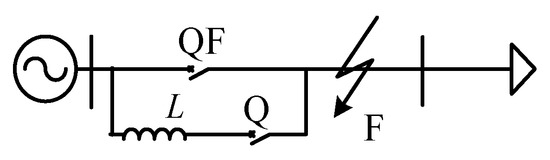
Figure 1.
Equivalent model of additional inductance of distribution network.
Where L is the additional inductance of the system, Q is the auxiliary switch, and QF is the line circuit breaker, F is the point of failure.
The coordination scheme based on additional inductance proceeds, as follows: (1) During regular operation, both the main breaker QF and the auxiliary switch Q remained open, leaving the inductance disengaged. (2) In the distribution network’s small current neutral grounding mode, if a line fault occurs, QF trips due to protection actions (set according to the original line’s fault current settings). The QF circuit breaker on the power side trips. Afterward, close the switch Q to perform distance measurement. In the case of a single-phase earth fault in the line, the fault current experienced only a minimal increase, not exceeding the preset threshold, which permitted the faulty line to continue operating for a specified duration. For maintenance-related distance measurements, QF was tripped, and then switch Q was closed. Following the closing of switch Q to engage the additional inductance, the faulted line underwent a transient process before reaching a stable operating state with the fault, referred to as the post-protection stable process. To ensure that the main breaker QF has opened the circuit and there is no current, it is recommended that the auxiliary switch Q be closed 0.2 s after the action of the breaker QF. To improve effective measurement time, enhance phase measurement accuracy, and, at the same time, disconnection can be carried out in the shortest possible time, and the closing time of switch Q is 0.5 s [23].
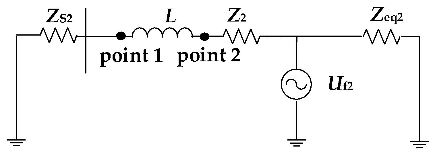
After collecting steady-state fault data, switch Q may be opened in preparation for maintenance. The symmetrical component method is used to analyze the post-protection steady-state fault information. When other types of faults occur (i.e., other than single-phase earth faults), the power supply remains operational. The inclusion of additional inductance can cause a significant fault current in the line due to other faults, but it also helps to limit this fault current. The positive and negative-sequence electrical quantities (voltage and current) from the three-phase line provide clear indications of significant fault information. In the event of a single-phase earth fault, the inductance’s inclusion allows the single power supply to continue operating, with a relatively low fault current flowing into the fault point. The power supply remains within the positive-sequence network, facilitating effective measurement of the faulted phase’s positive-sequence electrical quantities. Regarding the negative-sequence components, the equivalent negative-sequence network of the line is illustrated in Figure 2.
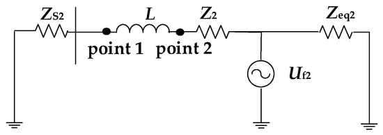
Figure 2.
The equivalent model of negative-sequence network after fault.
Where ZS2, Z2 and Zeq2 are the equivalent negative-sequence impedance on the power side, the line negative-sequence impedance and the equivalent negative-sequence impedance after the point of fault, and Uf2 is the negative-sequence power source. Points 1 and Points 2 are the two voltage measurement points in front of and behind the auxiliary inductor.
From the analysis of Figure 2, we can infer that the negative-sequence voltage decreases from the fault point along the line toward the grounding point on the power supply side, ultimately reaching zero. The negative-sequence voltage measured at point 2 is of a larger magnitude than that at point 1. Therefore, in this paper, the electrical quantity measurement point is designated as point 2. Without additional inductance, the impedance of the negative-sequence network along the line is represented by ZS2 and Z2, at which time points 1 and 2 can be considered identical. The negative-sequence voltage derived from the three-phase voltage at the line terminal is the result of voltage division across ZS2. If ZS2 is relatively small, the magnitude of the negative-sequence voltage at the line terminal will also be small, rendering the fault information less discernible. Hence, the addition of additional inductance effectively increases the measured magnitude of the negative-sequence voltage.
2.2. Identify the Supplementary Inductance
Following a fault in the system, the equivalent circuit of the faulted state network, based on the coordination scheme with additional inductance, is shown in Figure 3.
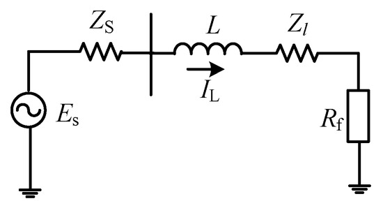
Figure 3.
The equivalent circuit of the faulted state network.
Where ZS, Zl and Rf are the equivalent impedance on the power side, the line impedance and the equivalent transition resistance after the point of fault, IL is the current flowing through the auxiliary inductor and ES is the power source. The short-circuit current, IL, during a fault, can be limited by the connected inductance as per the protective scheme described in this paper. Considering an extreme scenario near the busbars, where a three-phase short-circuit fault occurs with zero transition resistance—meaning the line is completely short circuited after the inductance—the short-circuit current IL can be calculated using Equation (1).
where ω0 is the angular velocity at the supply frequency. According to Equation (1), the auxiliary inductance can be derived as Equation (2).
Under these conditions, upon the introduction of inductance, the line will operate with faults for a certain period. To ensure the line’s safety, the current must be less than or equal to the rated current at this time. Additionally, to guarantee accurate collection of electrical quantities after a fault, the line current must be greater than or equal to the minimum value detectable by the current transformer. The range of short-circuit current IL is specified by Equation (3).
where represents the rated current, and represents the minimum detectable amplitude by the current transformer. Considering the uncertainty of the fault location and the suppressive effect of line resistance and additional inductance on the line current amplitude, it is recommended to keep the magnitude of IL as close as possible to the rated current.
2.3. Analysis of Coordinated Scheme Based on Additional Inductance
The monitoring equipment, FTU, can enable the collaboration and interaction between devices to implement coordinated plans. After a fault occurs, the inductance is connected to transition the line into a stable state of operation with the fault. Distance analysis is performed using steady-state data. In this coordination scheme, the distance measurement method that relies on steady-state data—as opposed to transient signal measurement methods that analyze specific moments—requires less demanding sampling equipment, is more cost effective, and extends the effective measurement time, thus improving the accuracy of electrical quantity measurements.
By setting the value of the auxiliary inductance appropriately, it is possible to limit the short-circuit current to near the rated value after a fault occurs, reducing measurement errors in the transformers. During asymmetrical fault conditions in the system, the auxiliary inductance will increase the amplitude of the negative-sequence component. This ensures an effective measurement of the steady-state value of the negative-sequence component in subsequent distance measurement methods, thus leveraging both the positive and negative-sequence components to eliminate errors caused by time asynchrony.
3. The Principle of Fault Location Method for Double-Ended Asynchronous Data
This paper employs a concentrated parameter π-type equivalent circuit on both sides of the fault point and analyzes the steady-state process after the protection operation. When the line experiences an asymmetric fault, the positive and negative-sequence networks of the system during a fault are analyzed using the symmetrical component method. The system has equal positive and negative-sequence impedances, as illustrated in Figure 4.
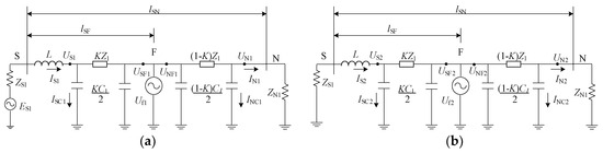
Figure 4.
The positive and negative-sequence networks of the system during a fault: (a) positive-sequence network; (b) negative-sequence network.
Where ZS1, Z1 and C1 are the equivalent positive-sequence impedance on the power side, the line positive-sequence impedance and the equivalent positive-sequence capacitance to ground, and ES is the power source. Uf1 and Uf2 are the positive-sequence power source and the negative-sequence power source. IS1 and IN1 are the positive-sequence currents at the S terminal and the N terminal. IS2 and IN2 are the negative-sequence currents at the S terminal and the N terminal. ISC1 and INC1 are the positive-sequence currents flowing through the ground capacitance at the S terminal and the N terminal, and ISC2 and INC2 are the negative-sequence currents flowing through the ground capacitance at the S terminal and the N terminal, respectively. US1, UN1, US2 and UN2 are the measured positive and negative-sequence voltages at the S terminal and N terminal. US1, UN1, US2 and UN2 are the positive and negative-sequence voltages of fault point F calculated by terminals S and N, respectively. The variable K represents the ratio of the distance from point S to the fault point F to the total length of the line. The positive and negative-sequence voltages on both sides of the line, the positive and negative-sequence currents at the busbar and the line impedance relationships are utilized to derive the positive and negative-sequence voltages at the fault point F, which can be expressed by Equation (4).
During the steady-state period, the fault point voltage can be determined separately using the positive and negative-sequence quantities of voltage and current from the respective networks. However, to calculate the fault distance using data from both ends, synchronous data are required. Taking the clock of the measurement device at terminal S as the reference, there may be a time asynchrony of 1–3 ms between the measurement device at terminal N and the device at terminal S. During the steady-state period, this timing error does not affect the amplitude, as the voltage magnitude remains constant. However, it does impact the accuracy of the phase angle measurement when calculating the phase angles of the two terminal voltages simultaneously. The phase angle influenced by this discrepancy is the asynchronous phase angle δd, and the synchronous voltage at terminal N can be expressed as Equation (5).
where n = 1, 2 represents positive sequence and negative sequence, respectively. U′N1 and U′N2 are the synchronous voltage at the N-terminal. UN1 and UN2 are the positive and negative-sequence voltages measured at the N-terminal.
When double-ended data synchronization occurs, the equality of the fault point voltage derived from both ends can be expressed by Equations (6) and (7).
In accordance with Equations (6) and (7), it is possible to construct Equation (8).
At this point, the phase angle error can be eliminated, and Equation (8) can be simplified. The fault location criterion as depicted in Equation (9) can be established.
By solving Equation (9), we can determine the ratio K between the fault distance and the total line distance, thereby obtaining the fault distance. Solving the quadratic complex equation may yield a spurious root. Given practical constraints, K should be a real number and not exceed 1. Nevertheless, measurement errors of electrical quantities and the process of solving sequence components inevitably introduce errors in magnitude and phase angle, thus affecting the quadratic complex equation of one variable-solving process, bringing the errors in the real and imaginary parts. Therefore, the criterion for determining K is presented in Equation (10).
where δl represents the maximum allowable absolute error in comparison to the total line length, for short distances in medium and low voltage distribution networks, the accuracy requirement can be set at 5% or selected based on the distance measurement accuracy requirements for different line scenarios.
The aforementioned analysis and solution to Equation (9) are only applicable to asymmetrical faults. For symmetrical faults such as three-phase short circuits, the faulted line has no negative-sequence component, only a positive-sequence component. In this scenario, the A-phase and B-phase voltages and currents at the S-terminal, along with the N-terminal voltage, can be used to substitute the positive and negative-sequence components in the equation. The analysis process and the formula remain essentially consistent after this substitution and can also eliminate the error in the phase angle. This aspect will not be further elaborated in this paper.
4. Simulation Analysis
To verify the correctness of the method proposed in this paper, simulations were conducted using PSCAD/EMTDC V4.6.2. The model of the 10 kV distribution system is depicted in Figure 5. The fault occurred at 0.5 s. After 0.3 s, the circuit breaker QF tripped due to the protection operation or manual disconnection. The switch Q was closed at 1.0 s, connecting the inductance, and the switch was opened at 1.5 s, disconnecting the inductance. The equivalent impedance of the voltage source was set at 0.55 + j0.32 Ω. The value of the auxiliary inductance can be calculated from Equation (2). in Section 2.2. In Equation (2), where = 10.5 kV, = = 100 rad/s and = 0.55 + j0.32 Ω. In Equation (3), = 0.35 kA and = 0.17 kA. These data can be used in Formula (2) to calculate the minimum value of the auxiliary inductance as 0.096 H and the maximum value as 0.193 H. Considering the analysis above, the inductance should be minimized to make the amplitude of the short-circuit current as close to the rated current as possible. For practical convenience, a value of 0.1 H can be chosen. The additional inductance was calculated to be 0.1 H, so an additional inductance of 0.1 H is installed in all three phases.
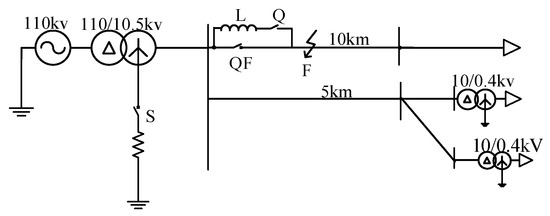
Figure 5.
Equivalent model of negative-sequence network after fault.
The line type is an overhead line. The unit length of distribution line parameters is presented in Table 1.

Table 1.
Unit length of distribution lines parameters.
At the midpoint of the 10 km route, a short circuit occurred between phases A and B, with a transition resistance of 10 Ω. The waveform of the A-phase current is shown in Figure 6.
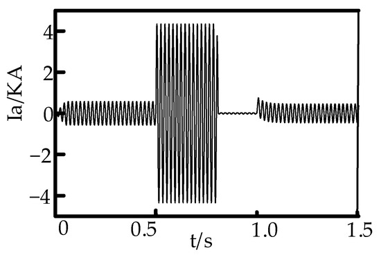
Figure 6.
The waveform of the A-phase current.
From Figure 6, it can be observed that, during normal operation, the amplitude of phase A current is 0.51 kA. At 0.5 s, a short circuit fault occurs, causing the A phase current to become 4.32 kA. At 0.8 s, circuit breaker QF opens, rapidly reducing the A phase current to 0. At 1.0 s, the auxiliary inductance is connected, and the current amplitude is 0.48 kA. Due to the auxiliary inductor, the short-circuit current is limited from 4.32 kA to 448 A. The negative-sequence voltages at measurement points 1 and 2 are shown in Figure 7.
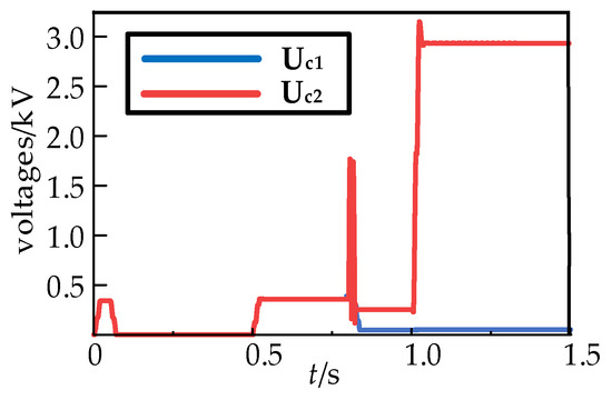
Figure 7.
The negative-sequence voltages at measurement points 1 and 2.
Analysis of Figure 7 indicates that the inductor is put into operation at 1.0 s, the negative-sequence voltages at measuring points 1 and 2 are 2.6 kV and 62 V, respectively. It can be observed that when the equivalent internal impedance on the system power supply side is small, the negative-sequence voltage at measuring point 2 is significantly greater than that at measuring point 1. Validated the methodology of Section 2.1 for the selection of measurement points. At this point, the coefficients in Equation (9) can be expressed as Equation (11).
By measurement and calculation, the following values are obtained: a = 35,073.74 + 15,370.71i and b = −17,541.83 − 7847.663i. Bringing the data into Equation (9) solves for k1 = 0.50182 + 0.00383i, k2 = 1.7541594 × 10⁷ + 7.8473940 × 10⁶i. Bringing the data into Equation (10), the spurious root k2 can be excluded, and k1 is considered the true root. Then, we calculated the fault location obtained by the algorithm as 5.0182 km. The accuracy of the methods described in this article has been thoroughly verified from various perspectives.
4.1. Analysis of the Impact of Fault Types and Fault Distances
To validate the accuracy of the method described in this paper, the steady-state vector method presented herein was compared with the results of the existing fast distribution fault transient time-domain method. In Reference [24], the formula for this time-domain method of fault location is given as Equation (12).
where K is the same as mentioned above, Lline and Rline are the total resistance and inductance of the measured line, and , , and are the voltages and currents at the ends of the line in the time domain.
The fault distance measurement results under different fault types and distances using the vector method and time-domain method are presented in Table 2. In the table, AB represents a two-phase short circuit, ABC denotes a three-phase short circuit and G indicates a ground fault. The transient resistance in all cases is 10 Ω. The absolute error is expressed as Equation (13).
where Xm is the fault location calculated by the algorithm and Xa is the actual fault location set by the system. The relative error is the absolute value of the percentage error in relative positioning, and it can be expressed as Equation (14).
Table 2.
Fault location results with different fault types and fault distances.
Upon analyzing the distance measurement results of the distribution network lines, it is evident from Table 2 that, for the same type of fault, as the fault location setting increases, the corresponding absolute error also increases. This trend is because Equation (13) shows that when the relative error is relatively stable, the absolute error rises with an increase in fault distance. The method accounts for factors such as ground capacitance and asynchronous time in the model, enhancing the accuracy of the method. The error primarily stems from signal measurement inaccuracies and the amplitude and phase angle in the Fourier transform, which are random in nature but have a relatively minor impact on the error. The maximum relative error is 0.36%, with an average relative error of 0.12%. The maximum absolute error obtained by the steady-state method is 18.8 m, signifying a high level of accuracy. In the case of single-phase ground faults, the average relative error obtained by the steady-state method is 0.24%. Conversely, the transient domain method exhibits a maximum absolute error of 25.5 m, a maximum relative error of 0.38%, an average relative error of 0.20% and an average relative error of 0.13% in the event of single-phase grounding faults. Given that during single-phase grounding faults, the steady-state fault current and negative-sequence voltage amplitude are relatively low, the measurement accuracy is somewhat lower compared to the transient method. However, for other types of faults, the distance measurement accuracy using this method is superior and overall better than that of the transient method. Moreover, under various fault locations and types, the relative error of the proposed method is less than 1%, fulfilling the requirements for fault distance measurement accuracy.
4.2. Analysis of the Impact of Transition Resistance
To verify the accuracy of the proposed method and assess the impact of high transition resistance on distance measurement, the results of fault location with different transition resistances are shown in Table 3. Here, the fault location, type and asynchronous phase angles are all consistent at 5 km, two-phase short circuit, and 0°, respectively.
Table 3.
Fault location results with different transition resistance.
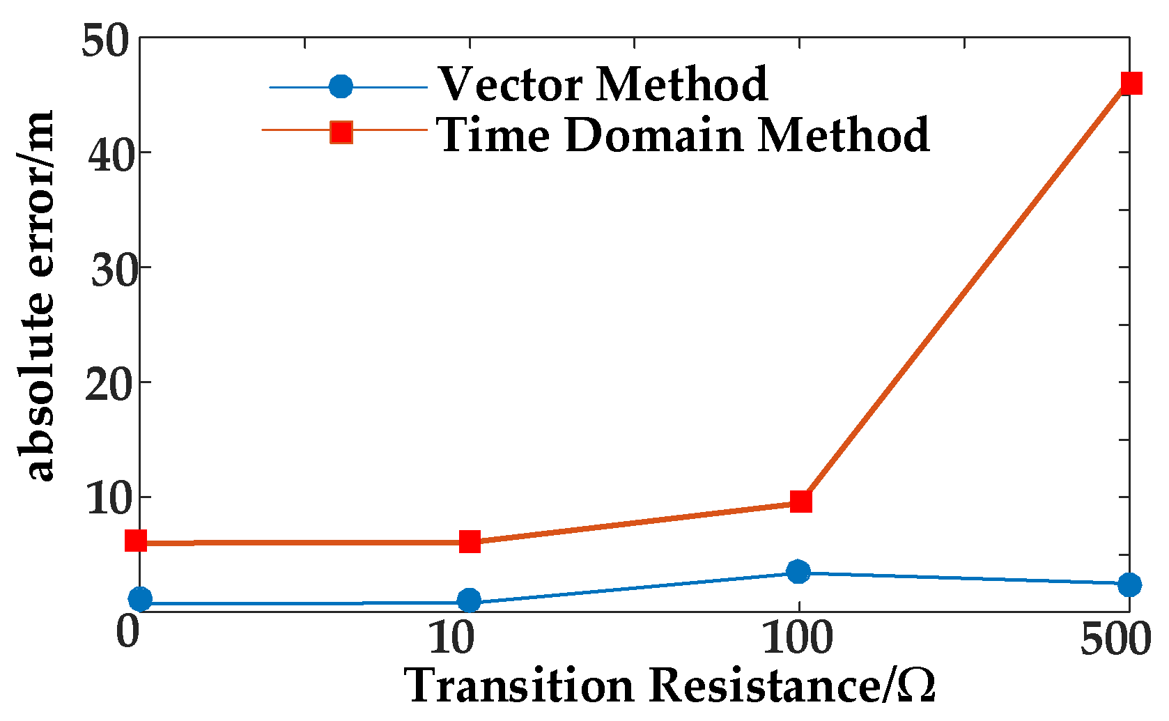
The analysis of the distance measurement results across varying transition resistances indicates that the steady-state distance measurement method proposed in this paper yields relatively low relative errors, meeting the requirements for accurate fault distance measurement. The relative errors of the method in this paper are all below 0.1%, demonstrating enhanced adaptability to high-resistance faults. The absolute error associated with different transition resistances is depicted in Figure 8.
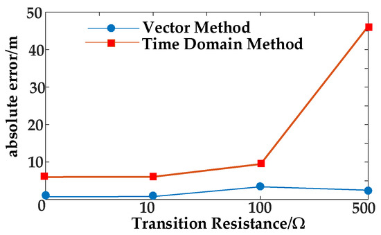
Figure 8.
Absolute error with different transition resistance.
An examination of Figure 8 reveals that when employing the time-domain method for fault distance measurement, the measurement error increases with an increase in transition resistance. This trend can be attributed to the fact that lower transition resistances result in higher fault currents, which are more straightforward to measure and calculate. Conversely, higher transition resistances produce smaller fault currents, complicating the measurement process and leading to larger computational errors, thus resulting in increased absolute error. However, when utilizing the method presented in this paper for fault distance measurement, the influence of transition resistance on absolute error is markedly reduced. The methodology leverages auxiliary inductance to ensure that, subsequent to a fault occurrence, the fault current at the measurement point approximates the rated current, thereby simplifying the measurement and calculation process. This approach minimizes the error introduced by the increased transition resistance, which can cause significant variations in fault current.
4.3. Analysis of the Impact of Asynchronous Phase Angle
To ascertain the accuracy of the distance measurement method under a spectrum of asynchronous phase angles, the unsynchronized time is denoted by t. The equation for converting between unsynchronized time and asynchronous phase angle is given by Equation (15). In the simulation, when solving Equation (9), the voltages affected by asynchronization (e.g., UN1, UN2) can be multiplied by different asynchronous phase angle values to simulate the effect of time asynchronization. We consider the timing errors discussed earlier, which range from 1 to 3 ms, that correlate to an approximate asynchronous phase angle span of 0–54°.
In experimental practice, these values cannot be determined (similar to the location of a line fault occurrence). Various sizes of asynchronous phase angle differences are used in the simulation in this paper to simulate this random situation. The simulation results corresponding to different asynchronous phase angles are outlined in Table 4, where the fault location, type and transient resistance are consistently set at 5 km, two-phase short circuit and 10 Ω, respectively.
Table 4.
Fault location results with different asynchronous phase angles.
Upon examining the distance measurement outcomes of both methodologies, as presented in Table 4, it becomes apparent that the distance measurement algorithm neglecting asynchronous phase angles suffers significantly under the influence of pronounced timing errors, with a maximum relative error reaching 13.72%. This starkly underscores the pronounced effect of timing errors and asynchronous phase angles on the accuracy of distance measurements. Conversely, the steady-state method discussed in this paper demonstrates substantial resilience, consistently maintaining a high degree of measurement accuracy. Figure 9 illustrates the absolute error variation in relation to different transition resistances.
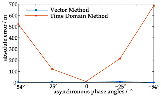
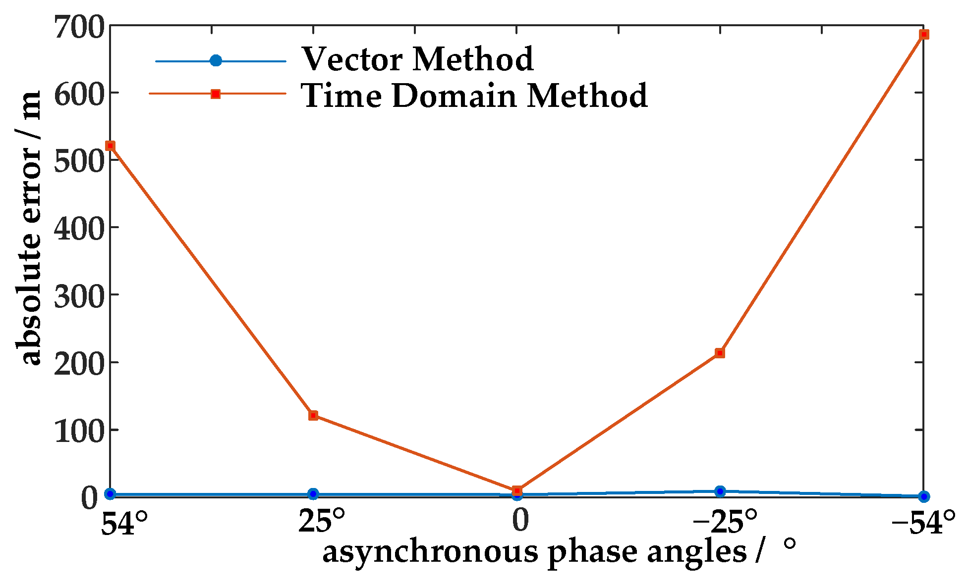
Figure 9.
Absolute error with different asynchronous phase angles.
An evaluation of the graph depicting absolute error reveals a direct correlation with the time-domain method; as the time asynchrony between the two endpoints widens, so does the absolute error. This increase in error is attributed to the method’s reliance on both ends’ data for fault distance measurement, where any time asynchrony between the two ends introduces data asynchrony during computations, and, consequently, errors. The graph indicates that as the absolute value of the time asynchrony increases (reflected as increasing asynchronous phase angles in the graph), the errors also increase. The method described in this paper eliminates the asynchronous phase angles stemming from different time factors through a calculated comparison of the positive and negative-sequence voltages, thus circumventing the associated adverse effects.
5. Discussion
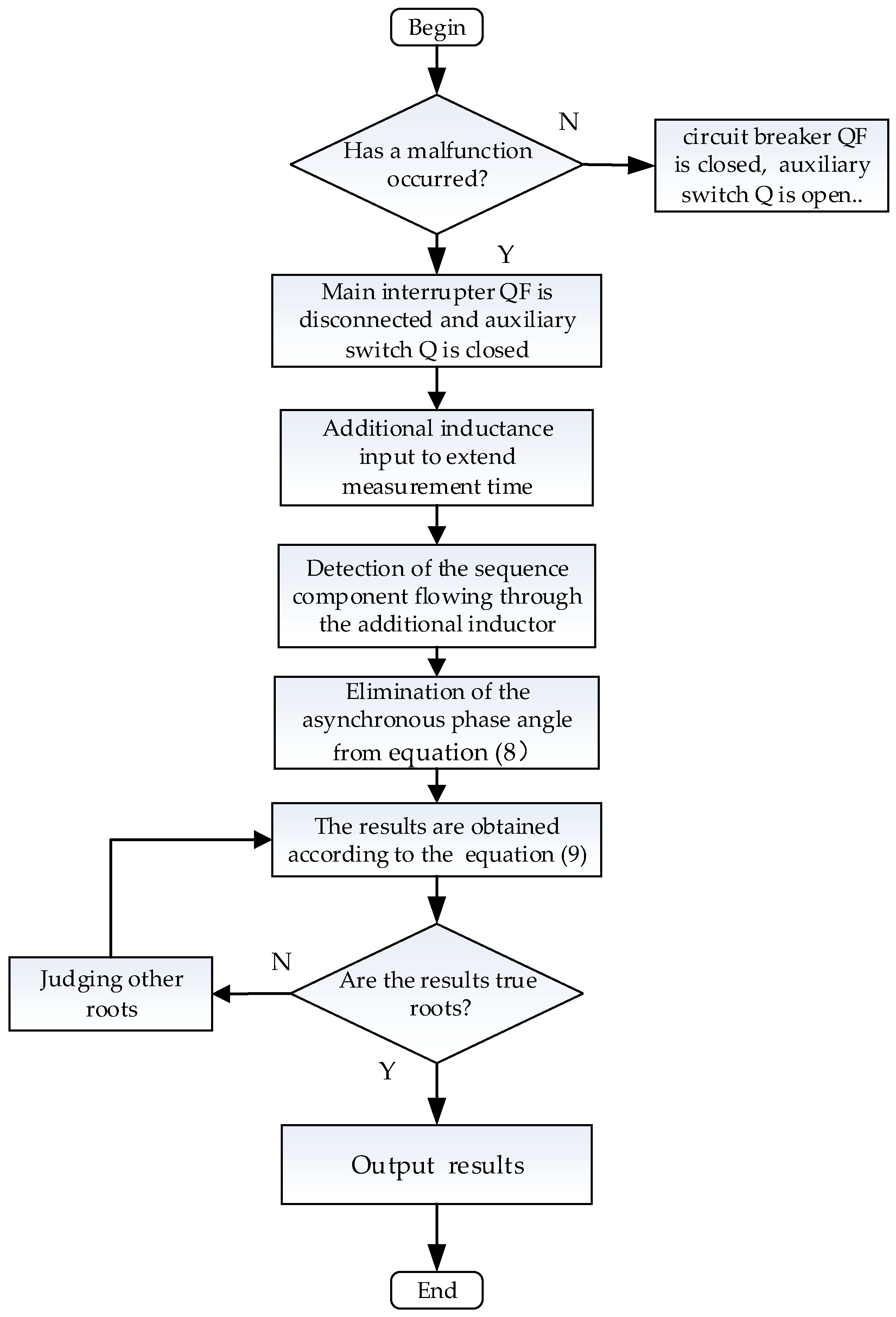
This paper presents a fault resolution strategy predicated on the use of additional inductance, incorporating strategies for additional inductance and elimination of timing errors. The procedural framework for fault location is delineated in Figure 10.
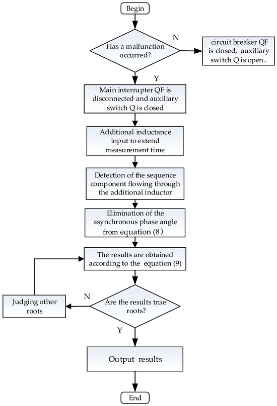
Figure 10.
Flowchart of fault location.
Where N and F respectively represent the judgments of no and yes, in order to proceed to the next action. As in determining whether or not a fault has occurred at the beginning, N is no fault occurred Y is yes a fault occurred.
The proposed fault distance measurement method for distribution lines based on additional inductance demonstrates robust immunity to variables such as transient resistance, fault type and fault distance. It delivers precise measurement results across a spectrum of asynchronous angles, fulfilling the stringent criteria set for fault distance measurement accuracy. In contrast to traditional transient distance measurement methods, the method expounded in this paper exhibits a broader range of applicability, particularly with respect to transient resistance and asynchronous angles. Nevertheless, in the context of actual line conditions that may involve intermittent arc grounding and numerous transient transition processes, prolonging the connection duration of the additional inductance may be necessary to ensure the capture of reliable steady-state data.
The asymmetry of the line and the unbalanced load can affect the measurement accuracy derived from PMU, rendering traditional symmetrical component methods fail. To address the issue of the asymmetry of the line, many high-voltage lines will undergo a fully transposed every 100 km (especially on EHV lines). This article did not consider the asymmetry of the line in the simulation and assumed that the load is balanced when a line fault occurs. This is because the method described in this article is used in the distribution network, where the line length is 10 km. Therefore, the line is relatively short (using a fully transposed can solve this problem). This approach eliminates loaded impedance from the calculations without the need to use specific values. Therefore, the asymmetry of the line and the unbalanced load has a certain impact on the method described in this paper, but its impact is relatively small.
This paper is specifically tailored to fault localization methods applicable to single-supply radial networks. The potential complexities introduced by the integration of ring networks and distributed energy resources represent prospective avenues for subsequent investigative endeavors.
6. Conclusions
A novel fault localization method is introduced, targeting the issue of inadequate phase measurement accuracy in the context of fault distance measurement in distribution networks. This issue is attributed to the short effective measurement time of the equipment and the time asynchrony between PMUs. The method is predicated on the implementation of additional inductance, offering a viable resolution to this prevalent issue.
- This paper proposes a fault-handling strategy that involves the strategic placement of an additional inductor subsequent to the online circuit breaker. This serves to extend the PMU’s effective measurement period, consequently bolstering the stability and accuracy of phase measurements;
- The strategy effectively converts the time asynchrony between devices into differences in asynchronous phase angles. By employing the symmetrical component method to derive the positive and negative-sequence voltages of the faulty line, the method facilitates a comparative analysis at the line terminal, effectively neutralizing the asynchronous phase angles and, by extension, diminishing the impact of asynchronous timing on fault localization accuracy;
- The accuracy of the proposed method, within the confines of a single power source radial model, has been substantiated through simulation. The findings corroborate the method’s capability to surmount the constraints imposed by asynchronous timing and inadequate precision of phasor measurement devices on localization accuracy. For circular network applications, including radial configurations, the coordination of circuit breakers at either end may be imperative for the successful adoption of the strategy delineated in this paper—an aspect earmarked for future research exploration.
Author Contributions
Methodology, Z.Y. and C.X.; Validation, Z.Y.; Formal Analysis, C.Y. and Z.Y. All authors have read and agreed to the published version of the manuscript.
Funding
Technology project at the Southern Power Grid Research Institute (SEPRI-K22B055).
Data Availability Statement
Data are contained within the article.
Conflicts of Interest
The authors declare no conflicts of interest.
References
- Guo, L.W.; Xue, Y.D.; Xu, B.Y.; Cai, Y.C.; Zhang, S.F. Research on effects of neutral grounding modes on power supply reliability in distribution networks. Power Syst. Technol. 2015, 39, 2340–2345. [Google Scholar]
- Cesar, G.; Ali, A. Fault location in active distribution networks containing distributed energy resources (DERs). IEEE Trans. Power Deliv. 2021, 36, 885–897. [Google Scholar]
- Yan, C.; Tao, L.; Wen, H.; Yao, Z.; Qing, X.; Hao, X.; Rui, L. Single-phase-to-earth fault location in distribution networks considering the distributed relations of the zero-sequence currents. Power Syst. Prot. Control. 2020, 48, 118–126. [Google Scholar]
- Qiao, J.; Yin, X.G.; Wang, Y.K.; Xu, W.; Tan, L.M. An accurate fault location method for distribution network based on active transfer arc-suppression device. Energy Rep. 2021, 7, 552–560. [Google Scholar] [CrossRef]
- He, J.H.; Zhang, M.; Luo, G.M.; Yu, B.; Hong, Z.Q. A fault location method for flexible dc distribution network based on fault transient process. Power Syst. Technol. 2017, 41, 985–991. [Google Scholar]
- Chen, X.; Jiao, Z.B. Accurate fault location method of distribution network with limited number of PMUs. In Proceedings of the China International Conference on Electricity Distribution (CICED), Tianjin, China, 17–19 September 2018. [Google Scholar]
- Sadeh, J.; Bakhshizadeh, E.; Kazemzadeh, R. A new fault location algorithm for radial distribution systems using modal analysis. Int. J. Electr. Power Energy Syst. 2013, 45, 271–278. [Google Scholar] [CrossRef]
- Deng, F.; Zeng, X.; Pan, L. Research on multi-terminal travelling wave fault location method in complicated networks based on cloud computing. Prot. Control Mod. Power Syst. 2017, 2, 2–19. [Google Scholar] [CrossRef]
- Lin, F.; Zeng, H. One-terminal fault location of single-phase to earth fault based on distributed parameter model of HV transmission line. Power Syst. Technol. 2011, 35, 201–205. [Google Scholar]
- Wang, B.; Dong, X.; Lan, L. Novel location algorithm for single-line-to-ground faults in transmission line with distributed parameters. IET Gener. Transm. Distrib. 2013, 7, 560–566. [Google Scholar] [CrossRef]
- Wang, G.; Xu, Z.L.; Liang, Y.S.; Gong, C. Single terminal time domain fault location method based on the similarity of square wave for arc grounding fault. Power Syst. Prot. Control. 2012, 40, 109–113. [Google Scholar]
- Liang, J.F.; Jing, T.J.; Niu, H.N.; Wang, J.B. Two-Terminal Fault Location Method of Distribution Network Based on Adaptive Convolution Neural Network. IEEE Access 2020, 8, 54035–54043. [Google Scholar] [CrossRef]
- Zhang, K.; Zhu, Y.; Zheng, Y. A fault location method for multi-branch hybrid transmission lines based on redundancy parameter estimation. Power Syst. Technol. 2019, 43, 1034–1040. [Google Scholar]
- Zhang, X.; Xu, Y.; Wang, Y.; Sun, Q.; Wang, Z.; Sun, Y. A double-end fault ranging algorithm based on parameter detection. Power Syst. Prot. Control. 2011, 39, 106–111. [Google Scholar]
- Wu, T.; Chung, C.Y.; Kamwa, I.; Li, J.; Qin, M. Synchro phasor measurement-based fault location technique for multi-terminal multi-section non-homogeneous transmission lines. IET Gener. Transm Distrib. 2016, 10, 1815–1824. [Google Scholar] [CrossRef]
- Xu, J.; Wang, Z.; Xia, P. Fault location algorithm for HV transmission lines based on samplings synchronized at both terminals by GPS. Guangdong Electr. Power. 2011, 24, 6–9. [Google Scholar]
- Ren, J.; Venkata, S.S.; Sortomme, E. An Accurate Synchrophasor Based Fault Location Method for Emerging Distribution Systems. IEEE Trans. Power Deliv. 2014, 29, 297–298. [Google Scholar] [CrossRef]
- Wang, L.; Liu, H.; Dai, L.V.; Liu, Y. Novel Method for Identifying Fault Location of Mixed Lines. Energies 2018, 11, 1529. [Google Scholar] [CrossRef]
- Shi, S.; He, B. Two-terminal fault location algorithm using asynchronous phase based on distributed parameter model. Power Syst. Technol. 2008, 32, 84–88. [Google Scholar]
- Sun, G.; Chen, R.; Han, Z.; Liu, H.; Liu, M.; Zhang, K.; Xu, C.; Wang, Y. Accurate Fault Location Method Based on Time-Domain Information Estimation for Medium-Voltage Distribution Network. Electronics 2023, 12, 4733. [Google Scholar] [CrossRef]
- Deng, W.; Lu, L.; Shi, J.; Yao, Z.; Qing, X.; Hao, X.; Rui, L. A fault location method for hybrid lines based on two-terminal asynchronous data. Power Syst. Technol. 2021, 4, 1574–1580. [Google Scholar]
- Yang, Z.; Xie, C.; Yin, C. Fault Location Method for Distribution Lines Based on Coordination of Primary and Secondary Devices. In Proceedings of the 2023 IEEE International Conference on Advanced Power System Automation and Protection (APAP), Xuchang, China, 8–12 October 2023; pp. 226–229. [Google Scholar]
- Liu, J.; Zhang, Z.; Wu, S. Fault processing with coordination of primary equipments and secondary devices. Power Syst. Prot. Control. 2019, 47, 1–6. [Google Scholar]
- Zhang, H.; Tang, M.; Cheng, Z. A fast time domain fault location method for single phase to ground fault in distribution network. Power Syst. Prot. Control. 2018, 46, 24–30. [Google Scholar]


Disclaimer/Publisher’s Note: The statements, opinions and data contained in all publications are solely those of the individual author(s) and contributor(s) and not of MDPI and/or the editor(s). MDPI and/or the editor(s) disclaim responsibility for any injury to people or property resulting from any ideas, methods, instructions or products referred to in the content. |
© 2024 by the authors. Licensee MDPI, Basel, Switzerland. This article is an open access article distributed under the terms and conditions of the Creative Commons Attribution (CC BY) license (https://creativecommons.org/licenses/by/4.0/).