Exact Sinusoidal Signal Tracking on a Modified Topology of Boost and Buck-Boost Converters

Abstract

This contribution presents new DC–DC Boost and Buck-Boost converter topologies to track sinusoidal signals in an exact form, that is, with zero error tracking. The proposed topology considers two DC–DC converters connected to the same load, which means that the converters are not in a cascade connection. To track the exact sinusoidal reference, the control algorithm is based on the indirect control algorithm and the harmonic balance method. The main contribution is to consider two control inputs that facilitate and permit canceling out the second harmonic generated by the nonlinearity of the model, and as a result there is a single frequency in the output. The result is such that the converters can track sinusoidal signals with exactly zero error. With this, there is a reduction in the potential negative effects on systems and equipment; some numerical results are presented to corroborate the proposal.

1. Introduction

The problem of tracking signals in DC–DC converters, particularly the tracking of sinusoidal signals, is of great importance due to the potential applications, particularly in UPS systems (Figure 1), where it is important to have zero error or at least a bounded error between the reference and the output signals. However, the inherent dynamical nonlinearities of the converters provide a variety of challenges; for instance, the tracking of sinusoidal signals with exactly zero error between the outputs and the reference signal. To this end, a design or redesign of standard typologies of the converters is proposed [1,2].

A common feature in the controller design process is to find the unstable tracking dynamics, i.e., systems whose internal dynamic becomes unstable when the outputs follow a given reference. The indirect control technique considers another output for which the internal dynamic becomes stable. Another problem occurs in this scenario: computing the new output’s reference target. Such a problem and the control technique are commonly found in the context of power converters. For current mode regulation and indirect control method in Boost and Buck-Boost converters, the reader is referred to [1]. In [2,3], a current reference, independent of a load parameter where a load disturbance exists is obtained, the scheme is an adaptive control technique, then an adaptive control for the sinusoidal tracking for the current inductor is used. In [4], a generalized predictive controller is designed to track and reject a biased sinusoidal signal for a discrete-time linear system; however, the Boost and Buck-Boost converter are, by nature, nonlinear systems, and this technique can not be implemented. An inverted topology DC–DC capable of giving a voltage that is bigger than the input is reported in [5], where a sliding mode controller is used and then a chattering problem is naturally presented. In [6], a stable inversion and robust tracking control method are applied to the Boost and Buck-Boost converters. A way to obtain a trigonometric approximation to the unstable periodic solution needed for the tracking problem for which the harmonic balance method is used is applied in [7], where the use of an adaptive scheme to eliminate load disturbance and sliding mode control is applied where, also, the chattering problem is presented. The increase in nonlinear loads in the electrical network induces harmonics and hence loss of energy, therefore the tracking of sinusoidal signals in an exact manner takes importance in the electronic design of power systems. This is also important in electrical engineering since the exact tracking reduces the presence of harmonics and reduces the high loss of energy [8,9,10]. The reader is referred to [11] for an overview of power converters, where it discusses the energy transfers between dynamic storage elements in lossless bilinear networks.

An n-phase interleaved Buck-Boost converter with a generalized steady-state model has been presented in [12]. In addition to the above discussed, it is well known that the DC–DC converters are a crucial device in applications of medium voltage in smart grids. The reader can see [13], where a transformerless DC–DC Boost-Resonant converter is presented, which is destined for the interconnection of medium- and high-voltage DC smart grids. The converters are also used in renewable energy applications as are presented in [14], where a new topology of the converter is presented and the design is such that the input current ripple of the introduced converter is very low, which is very desirable for renewable energy source applications. In solar energy system applications, the DC–DC converters also are used, as well pointed out in [15], and they are extensively used in electric vehicles, which the reader can see in [16], where a dual input Super-Boost DC–DC converter for a solar-powered electric vehicle is applied, among others. For instance, an application in a UPS system can be viewed in Figure 1; all these applications give us the importance of studying their control and how it can follow and exact sinusoidal reference signals.

On this note, we consider the problem of tracking a sinusoidal voltage reference given by $f\left(\tau \right)=A+Bsin\left(\omega \tau \right)$ by the converter’s output voltage in a new Boost and Buck-Boost topology in an exact manner, with zero error between the sinusoidal signal reference and the output voltage of the converter. A stable nonlinear system is determined to obtain the necessary inputs to follow the reference signal in an exact manner; to this end, a Boost and Buck-Boost topology is designed to provide two degrees of freedom in the input space. These topologies are shown in Figure 2, and the parallel connection between two converters to the same load can be seen, this allows us to increase the input space from one input to two inputs. This paper is organized as follows: In Section 2, the model of the new topology of the converter is obtained and the conditions on which the currents of the inductors follow a reference with zero error are derived, remarking that these references will be also sinusoidal signals. In Section 3, simulation results are given to show the effectiveness of the method and a MatLab Block diagram is provided to show the real performance of the converter. Finally, in the last section, we draw a few conclusions and future works that will be worked on.

2. Problem Statement and Model Description

2.1. Problem Statement

The main problem to attend to consists of controlling a DC–DC converter so that the voltage output tracks exactly, with the tracking error equal to zero as a sinusoidal signal. However, a second harmonic is produced in the output when a standard power DC–DC converter with one control input tracks a sinusoidal reference. Therefore, it is desirable to eliminate or cancel the second harmonic signal and obtain zero error in the tracking output signal. In this case, small signal modeling [17,18,19] is not considered because this technique is used for a linear system’s point of view, and in our case the problem is nonlinear. Thus, nonlinear techniques must be used, like Lyapunov theory and the LaSalle principle [20]. The new topology consists of adding a second stage to the standard converter so that the output of the second converter is connected to the load in the first converter to cancel out the second harmonic. It can be observed that the converters are connected in parallel form and are not two converters connected in cascade form; they are not one after the other (Figure 2). Typically, the cascade connection increases the voltage and then steps down the voltage in the regulated form [21]. In different forms, in this design, the converter is connected in parallel form and only works together to eliminate the second harmonic.

The dynamical model for a single DC converter has the following model:

$$\begin{array}{cc}\hfill \dot{x}& =1-(k+y)\overline{u}\hfill \\ \hfill \dot{y}& =-ay+x\overline{u}\hfill \end{array}$$

(1)

where $y\left(\tau \right)=\frac{v_C\left(t\right)}{V_{CC}}$${|}_{t=\tau \sqrt{LC}}$ is the scaled capacitor voltage in the scaled time variable $\tau =\frac{t}{\sqrt{LC}}$, $x\left(\tau \right)=\frac{i_L\left(t\right)}{V_{CC}}\sqrt{\frac{L}{C}}$${|}_{t=\tau \sqrt{LC}}$ is the scaled inductor current in the scaled time $\tau$, $\overline{u}$ is the control input defined by $\overline{u}=1-sw$, where $sw$ is the switched value that takes its values in the set $S=[0,1]$, where $sw=1$ if the switch is ON and $sw=0$ if it is OFF, a is the scaled parameter given by $a=\frac{1}{R}\sqrt{\frac{L}{C}}$ where R is the load, L is the inductance and C is the capacitance. If $k=0$ the model is for a Boost converter and if $k=1$ the model is for a Buck-Boost converter [1,2,3,7].

By multiplying the first equation in (1) by x and the second equation in (1) by $(k+y)$, the following differential equation is obtained:

$$\begin{array}{c}\hfill (k+y)(\dot{y}+ay)=x(1-\dot{x})\end{array}$$

(2)

The objective is that the output voltage $y\left(\tau \right)$ tracks a sinusoidal signal $f\left(\tau \right)=A+Bsin\left(\omega \tau \right)$ in an exact manner; however, note that from Equation (2), the product of the output ($y\left(\tau \right)$) produces a second harmonic. The proposed control in [2,3] makes the current track the reference with zero error, but in contrast, the voltage has the second harmonic component and tracks the target signal reference with a small error.

From Equation (2), when $y_{ss}\left(\tau \right)=f\left(\tau \right)=A+Bsin\left(\omega \tau \right)$ in a steady state and the reference signal for the current is given by Equation (3), then the solution of Equation (2) is not possible since it produces inconsistent nonlinear simultaneous equations to determine the parameters. The problem is that in Equation (2), it produces a second harmonic, and then, to solve Equation (2), it is necessary for a term of the second harmonic, and then we have five equations to fulfill. However, there are only three parameters on Equation (3) and it is impossible to solve the solution of the equations, given in the harmonic balance method. If one proposes an extra harmonic in Equation (3), the products in (2) produce more harmonics. Therefore, this procedure generates an infinite number of harmonics. Then, the topologies used in [1,2,3,7] only contain one DOF (degree of freedom) and using the harmonic balance method, result in an inconsistent system of equations to solve it; this implies neglecting some equations [1]. The reference current in [1,2,3,7] is taken as

$$\begin{array}{c}\varphi =\overline{A}+\overline{B}cos\left(\omega \tau \right)+\overline{C}sin\left(\omega \tau \right)\end{array}$$

(3)

Departing from the mathematical model of the converter Equation (2), the problem is to find a control input such that $y\left(\tau \right)\to f\left(\tau \right)>0$ where $f\left(\tau \right)=A+Bsin\left(\omega \tau \right)$ is a sinusoidal signal reference. From the above discussion, it is not possible since the product of sinusoidal signals increases the number of harmonics. To tackle this problem, a second control input is required, and then a new topology is proposed.

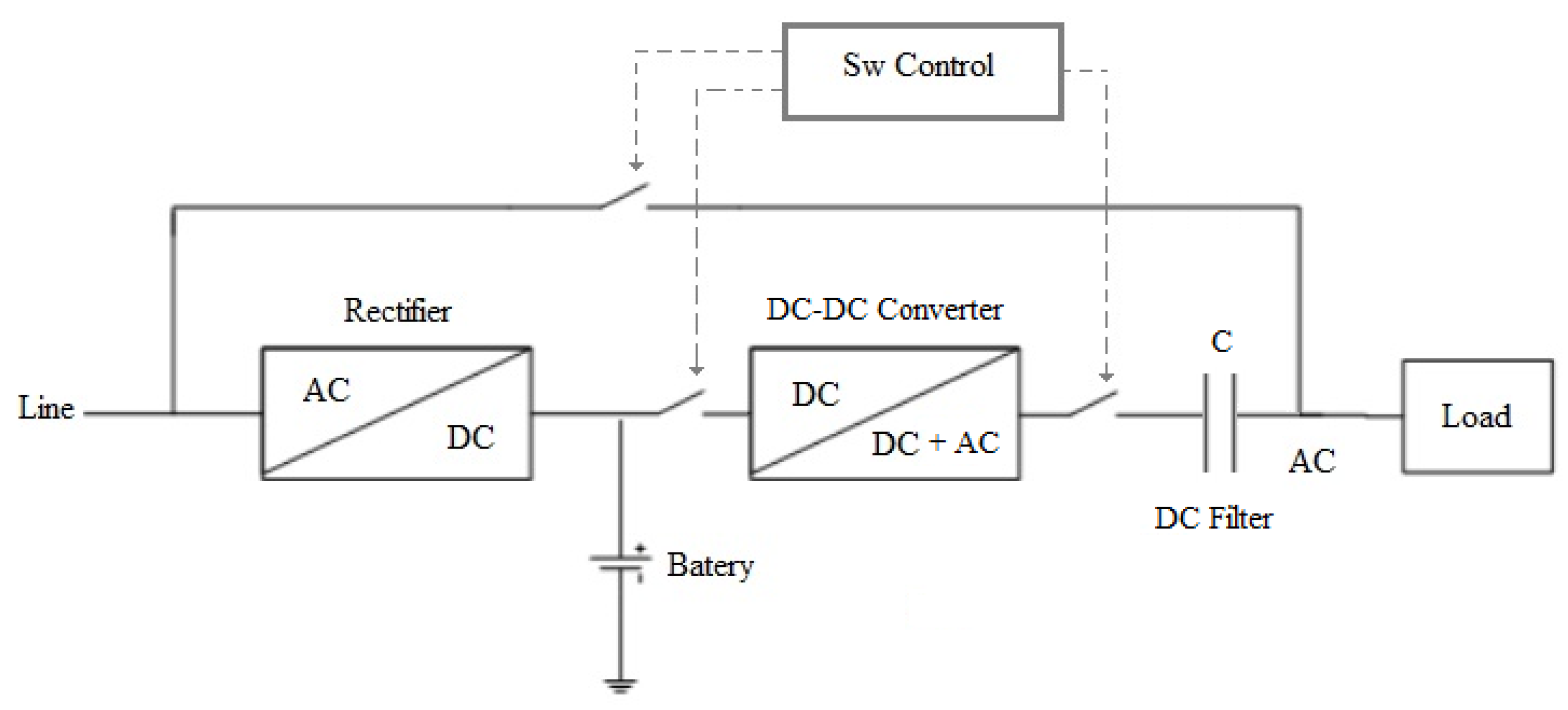
2.2. Model Description

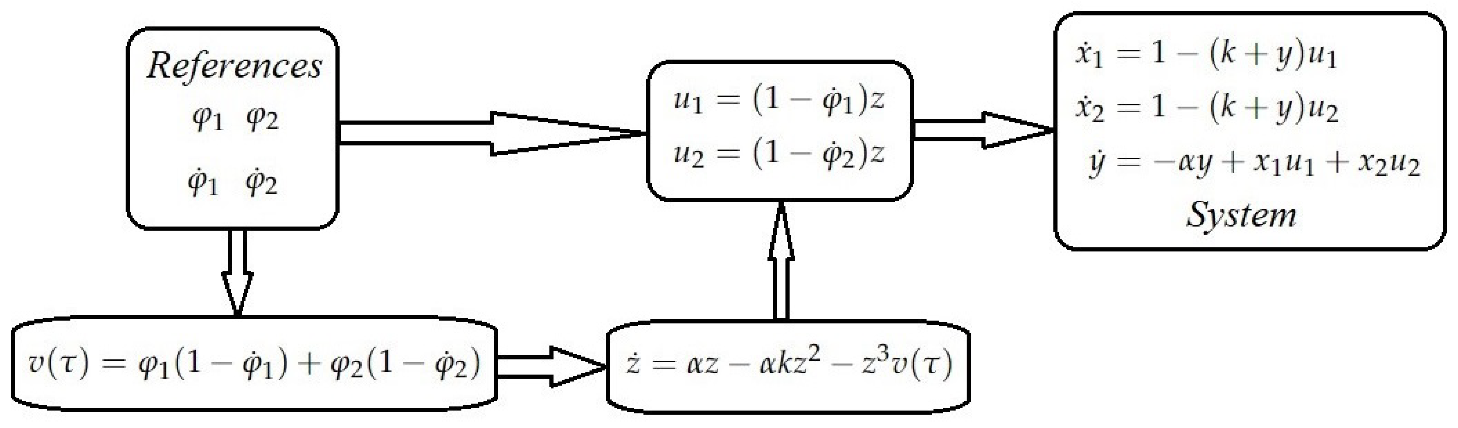
The main objective of this proposal is to control a DC–DC converter to track sinusoidal signals without a second harmonic. To this end, an improvement of the Boost and Buck-Boost topologies is performed. The main idea consists in generating a second current $i_2$ that permits a second degree of freedom and, therefore, a second control input that cancels the second harmonic produced by the model [1,3].

The new Boost and Buck-Boost topology converter circuits are shown in Figure 2, which consist of connecting two converters in parallel to a single load to obtain, according to the Kirchhoff current law, two current inputs in the voltage dynamics.

Concerning Figure 2, the dynamics of the DC–DC power converters are defined by the following differential equations:

$$\begin{array}{cc}\hfill L\frac{d{i}_1}{dt}& =v_C(s{w}_1-1)+V_{CC}[1+k(s{w}_1-1)]\hfill \\ \hfill L\frac{d{i}_2}{dt}& =v_C(s{w}_2-1)+V_{CC}[1+k(s{w}_2-1)]\hfill \\ \hfill C\frac{d{v}_c}{dt}& =i_1(1-s{w}_1)+i_2(1-s{w}_2)-\frac{v_C}{R}\hfill \end{array}$$

(4)

These equations are obtained as follows: From the circuit in Figure 2 it is clear that for $s{w}_x$ (switch is ON) the inductor is charging in both cases $k=1$ for Buck-Boost and $k=0$ for the Boost converter) and the capacitor discharges on the load. If $s{w}_x$ (switch is OFF) the inductors are discharging in an $RC$ circuit also in both cases. Once the inductors are charged, they are current sources and only apply the Kirchhoff current law to the $RC$ circuit. Considering the case ($k=0$) the voltage source is in series with the inductor, and in the other case ($k=1$) only the voltage source is disconnected and the inductor is the current source for the RC circuit. Thus, Equation (4) describes the dynamics of the proposed circuit, where $s{w}_1$ and $s{w}_2$ are the control signals that take their values in the set $S=$ [0,1], where $S=0$ means the state is open and when $S=1$ the state is closed in the switches; the parameter k defines the type of converter, for a Boost converter $k=0$ and $k=1$ for a Buck-Boost converter. $v_C$, $i_1$, $i_2$, and $V_{CC}$ are the capacitor voltage, inductor currents, and input voltage, respectively, and t is the real time variable and $\tau$ is the scaled time variable. To simplify the analysis, the following change of variables is made (see [1]):

$$\begin{array}{c}{x}_1=\frac{i_1}{V_{CC}}\sqrt{\frac{L}{C}};x_2=\frac{i_2}{V_{CC}}\sqrt{\frac{L}{C}};\hfill \\ y=\frac{v_C}{V_{CC}};\tau =\frac{t}{\sqrt{LC}};\hfill \\ \alpha =\frac{1}{R}\sqrt{\frac{L}{C}};{\overline{u}}_1=1-s{w}_1;{\overline{u}}_2=1-s{w}_2.\hfill \end{array}$$

(5)

the differential equations then become

$$\begin{array}{cc}\hfill {\dot{x}}_1& =1-(k+y){\overline{u}}_1\hfill \\ \hfill {\dot{x}}_2& =1-(k+y){\overline{u}}_2\hfill \\ \hfill \dot{y}& =-\alpha y+x_1{\overline{u}}_1+x_2{\overline{u}}_2\hfill \end{array}$$

(6)

where

$$\begin{array}{cc}\hfill {\dot{x}}_1=\frac{d{x}_1}{d\tau },{\dot{x}}_2=\frac{d{x}_2}{d\tau },\dot{y}& =\frac{dy}{d\tau }\hfill \end{array}$$

(7)

3. Main Result

The exact tracking is obtained by employing the two control inputs; therefore, we illustrate the procedure for designing the control inputs.

From Equation (6) solving for ${\overline{u}}_1$ and ${\overline{u}}_2$ and replacing these solutions in the last equation of (6), we have

$$(k+y)(\dot{y}+\alpha y)=x_1(1-{\dot{x}}_1)+x_2(1-{\dot{x}}_2)$$

(8)

It can be noted that the Boost and Buck-Boost converters need indirect control of the output voltage [1,3,7] because if direct control is used, the internal dynamics results in an unstable behavior for the inductor currents. Considering signals ${\phi }_1\left(\tau \right)$ and ${\phi }_2\left(\tau \right)$ as the reference for $x_1\left(\tau \right)$ and $x_2\left(\tau \right)$, respectively, then the control objective is that the output signals $x_1$ and $x_2$ track the reference signals ${\phi }_1$ and ${\phi }_2$ with zero error using a smooth controller. Substituting $x_1={\phi }_1$ and $x_2={\phi }_2$ in Equation (8), the output derivative is rewritten as follows:

$$\dot{y}=-\alpha y+\frac{{\phi }_1(1-{\dot{\phi }}_1)}{k+y}+\frac{{\phi }_2(1-{\dot{\phi }}_2)}{k+y}$$

(9)

The next change in variable $z={(k+y)}^{-1}$ is performed to show that the output variable is stable, and from Equation (9) the dynamics of $z\left(\tau \right)$ is given as follows:

$$\dot{z}=\alpha z-\alpha k{z}^2-z^{3}v\left(\tau \right)$$

(10)

With $v\left(\tau \right)={\phi }_1(1-{\dot{\phi }}_1)+{\phi }_2(1-{\dot{\phi }}_2)$. For the reference linear independent currents ${\phi }_1>0$, ${\phi }_2>0$ and $1-{\dot{\phi }}_1>0$, $1-{\dot{\phi }}_2>0$ with $z\left(0\right)>0$, then $z\left(\tau \right)$ tends to a stable limit cycle $\eta \left(\tau \right)={(k+\gamma \left(\tau \right))}^{-1}$. Taking the continuous control inputs $u_1$, $u_2$ (the mean of ${\overline{u}}_1$ and ${\overline{u}}_2$, respectively), and the continuous control inputs in steady state $u_{ss1}$ and $u_{ss2}$, then $u_{ss1}=(1-{\dot{\phi }}_1)\eta$, $u_{ss2}=(1-{\dot{\phi }}_2)\eta$. Thus, the scaled system (6) and the dynamics of $z\left(\tau \right)$ are implemented as follows:

$$\begin{array}{cc}\hfill {\dot{x}}_1& =1-(k+y)u_1\hfill \\ \hfill {\dot{x}}_2& =1-(k+y)u_2\hfill \\ \hfill \dot{y}& =-\alpha y+x_1{u}_1+x_2{u}_2\hfill \\ \hfill \dot{z}& =\alpha z-\alpha k{z}^2-z^{3}v\left(\tau \right)\hfill \\ \hfill u_1& =(1-{\dot{\phi }}_1)z\hfill \\ \hfill u_2& =(1-{\dot{\phi }}_2)z\hfill \end{array}$$

(11)

and it is obtained that $u_1\to u_{ss1}$, $u_2\to u_{ss2}$, $x_1\to {\phi }_1$, $x_2\to {\phi }_2$, $y\to \gamma$. To prove this assertion, consider the error signals $e_{x_1}=x_1-{\phi }_1$, $e_{x_2}=x_2-{\phi }_2$, and $e_y=y-\gamma$, and construct the error dynamics systems on the steady state of $z\left(\tau \right)$:

$$\begin{array}{c}{\dot{e}}_{x_1}=-\frac{1-\dot{{\phi }_1}}{k+\gamma }{e}_y\hfill \\ {\dot{e}}_{x_2}=-\frac{1-\dot{{\phi }_2}}{k+\gamma }{e}_y\hfill \\ {\dot{e}}_y=-\alpha e_y+\frac{1-\dot{{\phi }_1}}{k+\gamma }{e}_{x_1}+\frac{1-\dot{{\phi }_2}}{k+\gamma }{e}_{x_2}\hfill \end{array}$$

(12)

Taking the Lyapunov function $V\left(e\right)=e_{x_1}^2+e_{x_2}^2+e_y^2$, which is positive definite and radially unbounded, its derivative results in $\dot{V}\left(e\right)=-2\alpha e_y^2$. Therefore, $e_{x_1}$, $e_{x_2}$, and $e_y$ are bounded, then the invariant set is $\Omega =\left\{(e_{x_1},e_{x_2},e_y)|e_y=0\right\}$, and considering the linear independence of ${\dot{\phi }}_1$ and ${\dot{\phi }}_2$, then $e_{x_1}\to 0$ and $e_{x_2}\to 0$. Then, by the LaSalle Theorem, it is concluded that all error systems tend to zero, and according to the persistence excitation theory, the convergence is exponential [20].

Note that ${\phi }_1$ and ${\phi }_2$ could be any linear independent functions of time and if ${\phi }_1>0$, ${\phi }_2>0$ and $1-{\dot{\phi }}_1>0$ $1-{\dot{\phi }}_2>0$, then with implementing (11), it is obtained that $x_1\to {\phi }_1$, $x_2\to {\phi }_2$, and $y\to \gamma$.

With the additional degree of freedom proposed in this work (for the input space) in the Boost and Buck-Boost topology converters, it is possible to balance Equation (8). In other words, a number of variables greater than equations are obtained; for observing this fact, let ${\phi }_1=D_1+E_{1}cos\left(\omega \tau \right)+F_{1}sin\left(\omega \tau \right)$ and ${\phi }_2=D_2+E_{2}cos\left(\omega \tau \right)+F_{2}sin\left(\omega \tau \right)$ be the current references, and $\gamma =f\left(\tau \right)=A+Bsin\left(\omega \tau \right)$ be the reference voltage that is applied in the harmonic balance method in Equation (8). Then, solving the constants for the equality

$$(k+f)(\dot{f}+\alpha f)={\phi }_1(1-{\dot{\phi }}_1)+{\phi }_2(1-{\dot{\phi }}_2)$$

(13)

the next set of nonlinear equations with $A_0=(A^2+kA+\frac{1}{2}{B}^2)$ is obtained

$$\begin{array}{c}\\ \hfill D_1+D_2& =\alpha A_0\hfill \\ \hfill F_1+F_2+\omega D_1{E}_1+\omega D_2{E}_2& =\alpha B\left(2A+k\right)\hfill \\ \hfill E_1+E_2-\omega D_1{F}_1-\omega D_2{F}_2& =B\omega \left(A+k\right)\hfill \\ \hfill E_1^2+E_2^2-F_1^2-F_2^2& =B^2\hfill \\ \hfill \omega E_1{F}_1+\omega E_2{F}_2& =\frac{1}{2}\alpha B^2\hfill \end{array}$$

(14)

Here, the first equation in (14) corresponds to the constant terms of the harmonic balance method, the second and third correspond to the first harmonic sine and cosine functions coefficients, respectively, and fourth and fifth equations correspond to the second harmonic sine and cosine function coefficients, respectively.

Let the value

$$\omega =\sqrt{2}\sqrt{\frac{2A+k}{A_o\left(A+k\right)}}$$

(15)

Then, take $D_1=D_2=\frac{1}{2}\alpha A_0$; $B_1=A+k$; $E_1=B_{1}B\omega -E_2$; $F_1=\frac{\alpha B^2}{2\omega \left(B_{1}B\omega -2E_2\right)}$; and $F_1=-F_2$. Thus, the currents references are

$${\phi }_1=\frac{1}{2}\alpha A_0+\left(B_{1}B\omega -E_2\right)cos\left(\omega t\right)+\frac{\alpha B^2}{2\omega \left(B_{1}B\omega -2E_2\right)}sin\left(\omega t\right)$$

(16)

$${\phi }_2=\frac{1}{2}\alpha A_0+E_{2}cos\left(\omega t\right)-\frac{\alpha B^2}{2\omega \left(B_{1}B\omega -2E_2\right)}sin\left(\omega t\right)$$

(17)

and solving the following equation

$${(B_{1}B\omega -E_2)}^2+E_2^2-\frac{{\alpha }^2{B}^4}{2{\omega }^2{\left(B_{1}B\omega -2E_2\right)}^2}=B^2$$

(18)

We found the necessary values for $E_2$ and finally the reference currents ${\phi }_1$ and ${\phi }_2$ to obtain the reference voltage $f\left(\tau \right)=A+Bsin\left(\omega \tau \right)$. We also observed the linear independence of $\dot{{\phi }_1}$ and $\dot{{\phi }_2}$ and that $y\left(\tau \right)\to f\left(\tau \right)=\gamma$ as we showed previously.

From the above discussion, the second degree of freedom in the input allows us to obtain an exact tracking of the sinusoidal reference. The block diagram of the proposed algorithm is shown in Figure 3. We first calculate the signals ${\phi }_1$ and ${\phi }_2$ and their derivatives; with these signals we obtain the signal $v\left(t\right)={\phi }_1(1-\dot{{\phi }_1})+{\phi }_2(1-\dot{{\phi }_2})$. With this signal, we perform the nonlinear differential equation to obtain $z\left(t\right)$ and finally obtain the control signals $u_1$ and $u_2$, and with these signals obtain the signals to control the switches as $s{w}_1=1-u_1$ and $s{w}_2=1-u_2$.

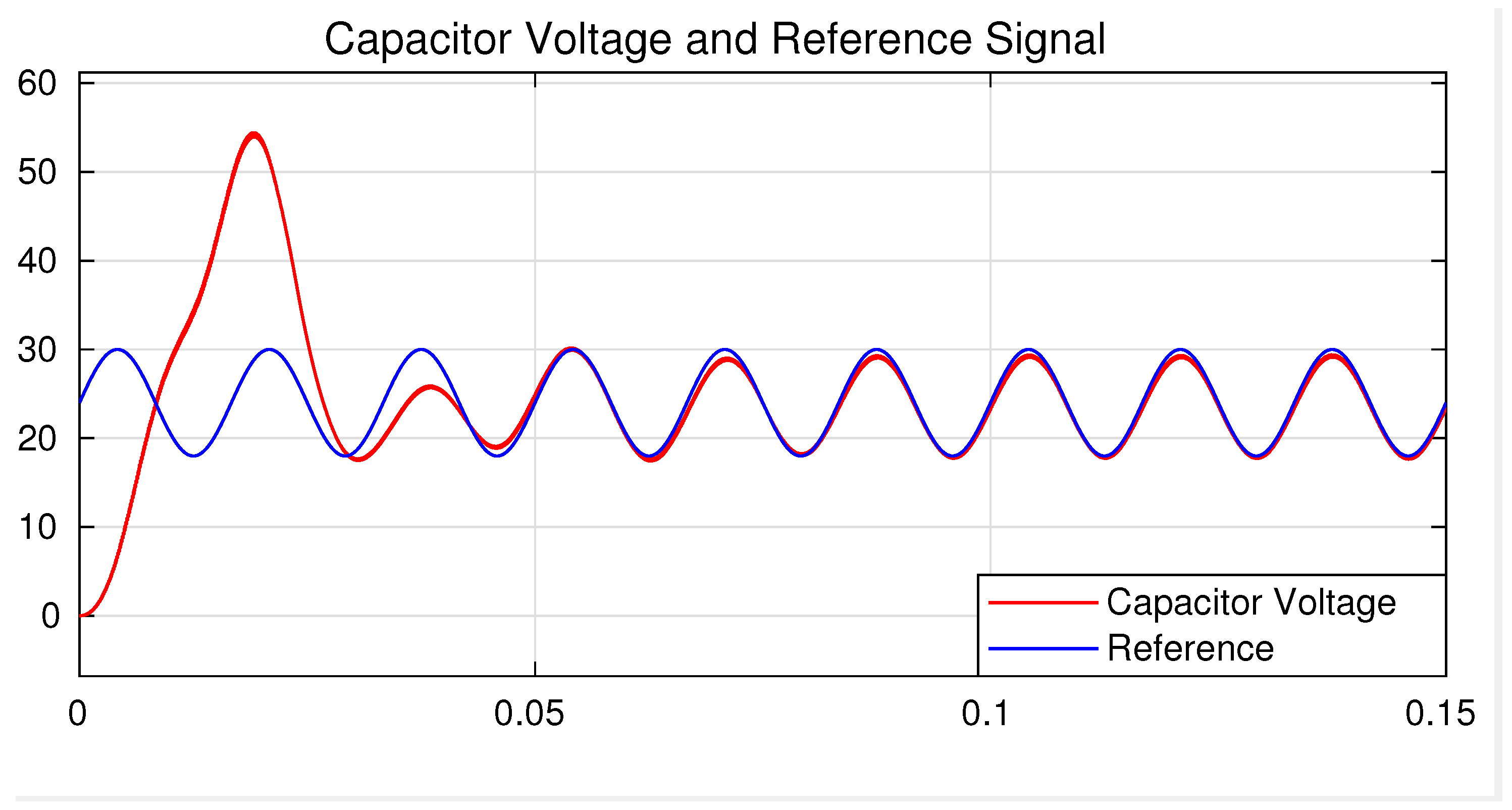
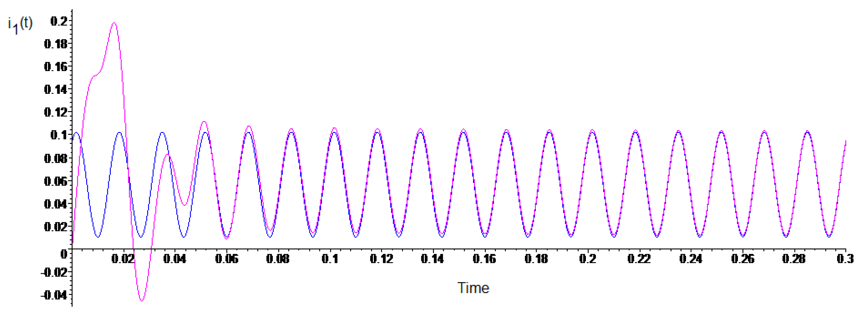
4. Simulation Results

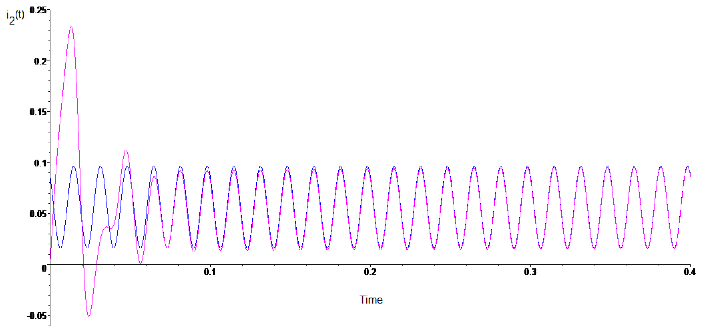
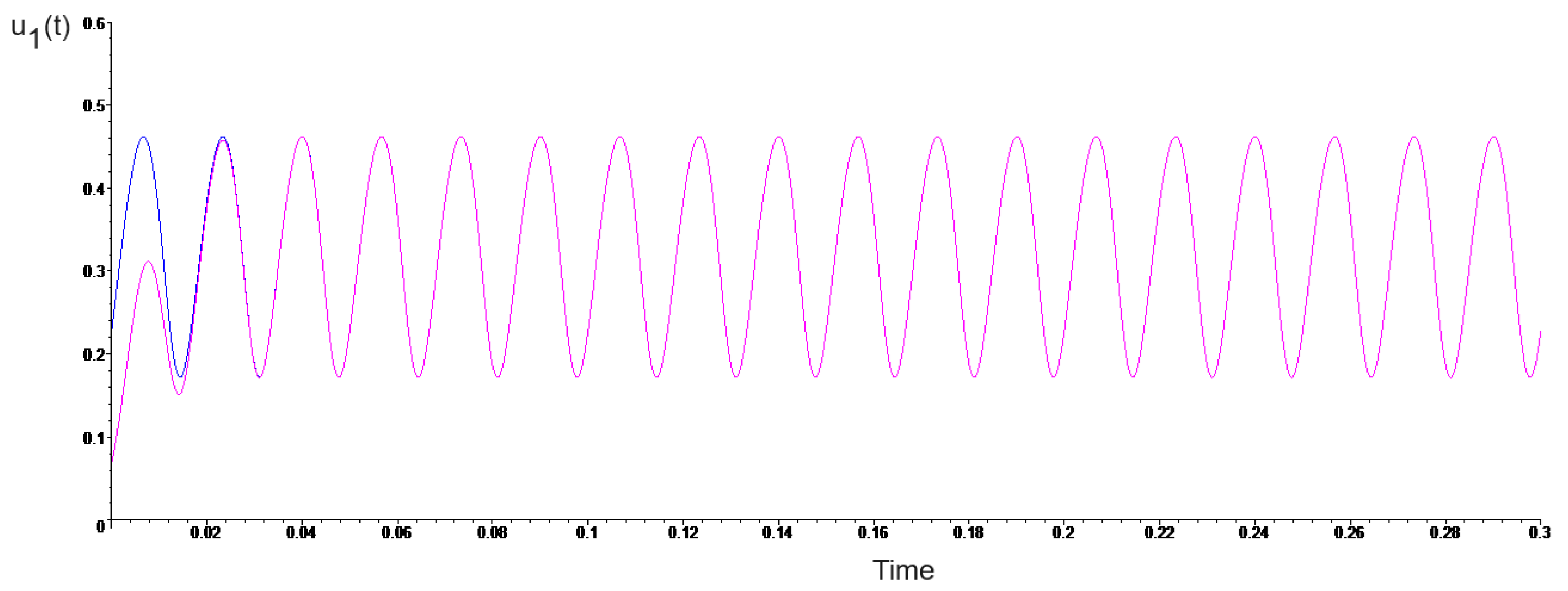
4.1. Single Phase Exact Sinusoidal Tracking

This section presents the results of the exposed dynamics system; the signal reference for the output voltage is $f\left(\tau \right)=2+0.5$$sin\left(\omega \tau \right)$. Consider the last results in the previous section and the initial conditions $z\left(0\right)=0.1$, $y\left(0\right)=0$, $x_1\left(0\right)=0$, and $x_2\left(0\right)=0$ with the values of the functions as:

$$\begin{array}{cc}\hfill f\left(\tau \right)& =A+Bsin\left(\omega \tau \right)\hfill \\ \hfill {\phi }_1\left(\tau \right)& =D_1+E_{1}cos\left(\omega \tau \right)+F_{1}sin\left(\omega \tau \right)\hfill \\ \hfill {\phi }_2\left(\tau \right)& =D_2+E_{2}cos\left(\omega \tau \right)+F_{2}sin\left(\omega \tau \right)\hfill \end{array}$$

(19)

and parameters $\alpha =0.3$, $A=2$, $B=0.5$, $k=1$, $\omega =0.7377111133=120\pi \sqrt{LC}$, $A_0=6.125$, $C=1000$ $\mathsf{\mu }$f, $L=3.82922$ mH, $D_1=D_2=\frac{\alpha A_0}{2}=0.91875$, $E_1=0.6124359343$, $E_2=0.4941307357$, $F_1=0.4296760164$, $F_2=-0.4296760164$, $V_{CC}=12$ V, $f_r=60$ Hz, and $R=652.2798$$\Omega$. In Figure 4 is shown the tracking output capacitor voltage $V_c\left(t\right)$ and reference $R_{vc}\left(t\right)=24+6sin\left(120\pi t\right)=V_{CC}f\left(\frac{t}{\sqrt{LC}}\right)$ obtained through the application of continuous input $u_1,u_2$. In Figure 5 is shown the block diagram performed in MatLab to simulate the proposed circuit. In Figure 6 we see the capacitor voltage obtained for the MatLab circuit; in this case there exists a small error due to the switching process, which is not a continuous process, although the tracking voltage is very acceptable. In this example, the switching frequency of PWM device is $f_s=10$ kHz; the current tracking $i_1\left(t\right),i_2\left(t\right)$ and references signals are shown in Figure 7 and Figure 8, respectively. Also, the continuous input signals $u_1,u_2$ can be seen in Figure 9 and Figure 10.

Remark 1. 

At this point, we must say that really the steady state of the inputs have an infinite number of harmonics because really the steady state of these signals is $u_{xss}\left(t\right)=\frac{1-\dot{{\phi }_x}\left(t\right)}{k+f\left(t\right)}$.

If we would like to measure the time constant, it is possible to measure the error and consider the $2\%$ criterion (4 $\tau$ ’s) to obtain the time constant for the voltage that results as ${\tau }_v=0.0204seg$, and for current response we have ${\tau }_i=0.0835seg$.

We summarize the comparison of some results in this context in the following

Table 1. Comparison of different algorithms.

Reference	Harmonics on $\mathit{y}\left(\mathit{\tau }\right)$	Restriction on B
[1]	Yes	Yes
[2]	Yes	Yes
[3]	Yes	Yes
Actual Result	No	No

.

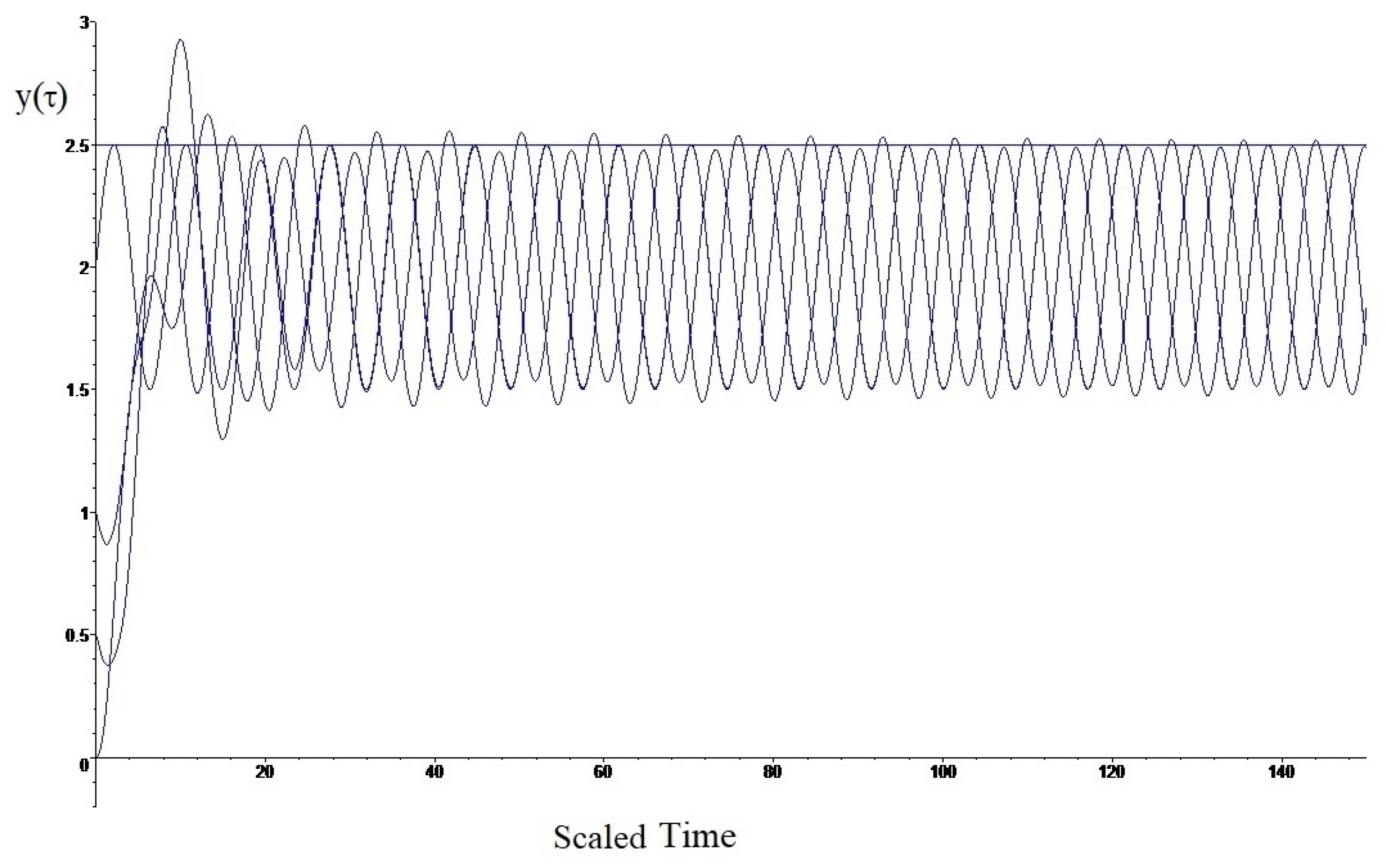
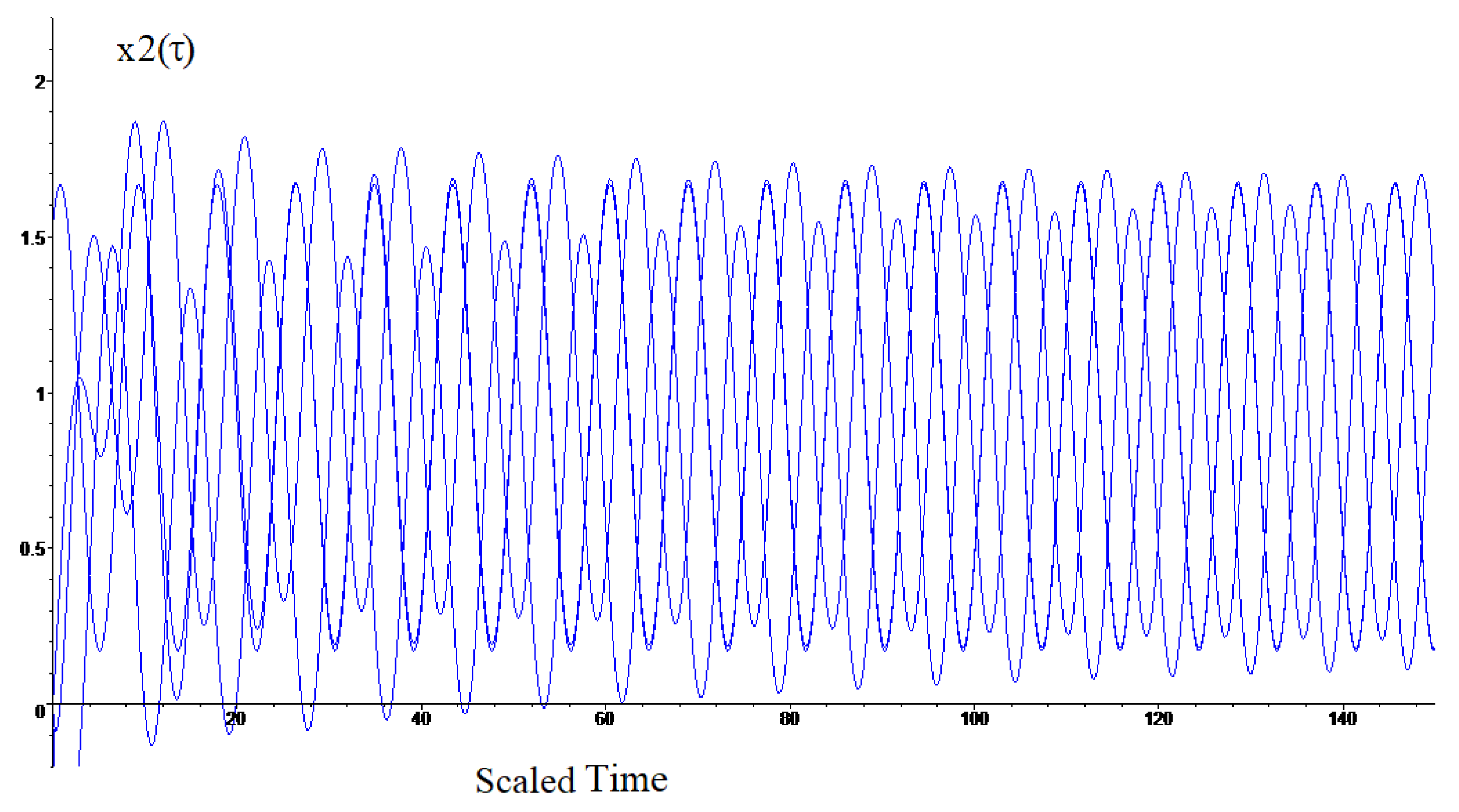
4.2. Tri-Phase Exact Sinusoidal Tracking

In this subsection, a generation of a tri-phase sinusoidal signal is reproduced using the proposed algorithm. The circuit scheme for the tri-phase sinusoidal signal generator is in Figure 11, and we can see the replication of the converter three times. The parameters of the circuits are the same as in the single-phase case; however, the parameter for the phase between them is different, that is, the phase angle between signals is $2\pi /3$ rad. It is important to note that the three input voltages $V_{CC}$ are considered the same source; however, these voltages could be different to obtain a greater current capacity. The important part of this system is that the rotatory magnetic field in the induction motors is obtained with zero harmonics. Figure 12 illustrate the tri-phases voltages and Figure 13 and Figure 14 stand for the currents in the circuit systems and also exactly track the sinusoidal references obtained for these currents.

5. Conclusions

In this paper, we present a different topology to exactly track the output voltage of the DC–DC Boost and Buck-Boost power converters to some biased sinusoidal signal, which consists of connecting the DC–DC converters to the same load, which is not a classical cascaded form. Then, to accomplish the signal tracking, a new way to generate the current references is proposed. For the tracking objective, it is compulsory to cancel a second harmonic. This requires a second input in the dynamics of the voltage; then, from the converter connection a node in the capacitor is included. According with the Kirchhoff currents law, this produces a sum in the currents; then, a sum of control inputs is obtained given the second degree of freedom in the control space. The proposed controller uses a nonlinear model to obtain the exact inputs necessary to obtain zero error tracking between the currents and, with this tracking of the currents, we obtain an exact tracking of an exact biased sinusoidal voltage in the load. Another important point is that the circuit configuration is not a cascaded one, since it is necessary to have two currents in the voltage dynamics, and this is not possible in a cascaded circuit. The proposal is such that it can be used to generate tri-phase sinusoidal signal tracking. For future work with the DC–DC power converters for exact sinusoidal tracking, a modification of the circuit converter would be proposed to have two inputs with only one converter.

References

1. Fossas-Colet, E.; Olm-Miras, J.M. Asymptotic Tracking in DC-DC Nonlinear Power Converters. Discret. Contin. Dyn. Syst. Ser. B 2002, 2, 295–307. [Google Scholar] [CrossRef]
2. Obregón-Pulido, G.; Solis-Perales, G.; Meda-Campaña, J.A.; Vega-Gómez, G.A.; Ruiz-Velázquez, E. Energy Considerations for Tracking in DC to DC Power Converters. Math. Probl. Eng. 2019, 2019, 1098243. [Google Scholar] [CrossRef]
3. Obregón-Pulido, G.; Nuño, E.; Castañeda, K.; De-Gyves, A. An Adaptive Control to Perform Tracking in Dc to DC Power Converters. In Proceedings of the 7th Conference on Electrical Engineering, Computing Science and Automatic Control, Tuxtla Gutierrez, Mexico, 8–10 September 2010; pp. 188–191. [Google Scholar]
4. Cordero, R.; Estrabis, T.; Gentil, G.; Caramalac, M.; Suemitsu, W.; Onofre, J.; Brito, M.; dos Santos, J. Tracking and Rejection of Biased Sinusoidal Signals Using Generalized Predictive Controller. Energies 2022, 15, 5664. [Google Scholar] [CrossRef]
5. Caceres, R.O.; Barbi, I. A Boost DC-AC converter: Analysis, design and experimentation. IEEE Trans. Power Electron. 1999, 14, 134–141. [Google Scholar] [CrossRef]
6. Olm, J.M.; Ros, X.; Shtessel, Y.B. A Stable inversion-based robust tracking control in DC-DC nonlinear switched converters. In Proceedings of the 48th IEEE Conference on Decision and Control and 28 Chinese Control Conference, Shanghai, China, 15–18 December 2009; pp. 2789–2794. [Google Scholar]
7. Fossas, E.; Olm, J.M.; Zinober, A.S.I. Robust Tracking Control of DC-to-DC Nonlinear Power Converters. In Proceedings of the 2004 43rd IEEE Conference on Decision and Control (CDC) (IEEE Cat. No.04CH37601), Nassau, Bahamas, 14–17 December 2004; pp. 5291–5296. [Google Scholar]
8. Ghorbani, M.J.; Mokhtari, H. Impact of Harmonics on Power Quality and Losses in Power Distribution Systems. Int. J. Electr. Comput. Eng. 2015, 5, 166–174. [Google Scholar] [CrossRef]
9. Harrison, A. The Effects of Harmonics on Power Quality and Energy Efficiency; Technological University Dublin: Dublin, Ireland, 2010. [Google Scholar]
10. Singh, R.; Singh, A. Energy loss due to harmonics in residential campus—A case study. In Proceedings of the 45th International Universities Power Engineering Conference UPEC2010, Cardiff, UK, 31 August–3 September 2010; pp. 1–6. [Google Scholar]
11. Sira-Ramirez, H. Sliding Motions in Bilinear Switched Networks. IEEE Trans. Circ. and Syst. 1987, 34, 919–933. [Google Scholar] [CrossRef]
12. Sarwar, A.; Shahid, A.; Hudaif, A.; Gupta, U.; Wahab, M. Generalized State Space Model for a n-Phase Interleaved Buck-Boost Converter. In Proceedings of the 4th IEEE Utar Pradesh Section International Conference of Electrical, Computer and Electronics (UPCON) GLA University, Mathura, India, 26–28 October 2017; pp. 62–67. [Google Scholar]
13. Anaya-Ruiz, G.A.; Robles, D.R.; Caballero, L.E.U.; Moreno-Goytia, E.L. Design and prototyping of transformerless DC-DC converter with high voltage ratio for MVDC applications. IEEE Lat. Am. Trans. 2023, 1, 62–70. [Google Scholar] [CrossRef]
14. Hasanpour, S.; Siwakoti, Y.P.; Blaabjerg, F. A New High Efficiency High Step-Up DC/DC Converter for Renewable Energy Applications. IEEE Trans. Ind. Electron. 2023, 70, 1489–1500. [Google Scholar] [CrossRef]
15. AW, N.H.; Siraj, S.F.; Ab Muin, M.Z. Modeling of DC-DC converter for solar energy system applications. In Proceedings of the 2012 IEEE Symposium on Computers & Informatics (ISCI), Penang, Malaysia, 18–20 March 2012. [Google Scholar]
16. Guru Kumar, G.; Sundaramoorthy, K.; Athikkal, S.; Karthikeyan, V. Dual input superBoost DC–DC converter for solar powered electric vehicle. IET Power Electron. 2019, 12, 2276–2284. [Google Scholar] [CrossRef]
17. Keong, N.P. Small Signal Modeling of DC-DC Power Converters Based on Separation of Variables. Master’s Thesis, University of Kentucky, Lexington, KT, USA, 2003. [Google Scholar]
18. Reddy, M.S.K.; Kalyani, C.; Uthra, M.; Elangovan, D. A Small Signal Analysis of DC-DC Boost Converter. J. Sci. Technol. 2015, 8, 1–6. [Google Scholar] [CrossRef]
19. Ayachit, A.; Kazimierczuk, M.K. Averaged Small-Signal Model of PWM DC-DC Converters in CCM Including Switching Power Loss. IEEE Trans. Circuits Syst. Ii Express Briefs 2019, 66, 262–266. [Google Scholar] [CrossRef]
20. Khalil, H.K. Nonlinear Systems, 3rd ed.; Prentice Hall: Upper Saddlfre River, NJ, USA, 2002. [Google Scholar]
21. Elkhateb, A.; Rahim, N.A.; Selvaraj, J. Cascaded DC-DC Converters as a Battery Charger and Maximum Power Point Tracker for PV Systems. In Proceedings of the 2013 International Renewable and Sustainable Energy Conference (IRSEC), Ouarzazate, Morocco, 7–9 March 2013. [Google Scholar]
Figure 1. Converter used in a UPS System.
Electronics 13 00793 g001
Figure 2. (a) Modified topology Boost converter. (b) Modified topology Buck-Boost converter.
Electronics 13 00793 g002
Figure 3. Block diagram of the proposed algorithm.
Electronics 13 00793 g003
Figure 4. Capacitor voltage V c ( t ) and reference signal R v c ( t ) = V c c f ( t L C ) .
Electronics 13 00793 g004
Figure 5. Block diagram for the proposed scheme.
Electronics 13 00793 g005
Figure 6. Capacitor voltage V c ( t ) and reference signal R v c ( t ) for circuit simulation, R v c ( t ) = 24 + 6 s i n ( 120 π t ) = V C C f ( t L C ) .
Electronics 13 00793 g006
Figure 7. Current output i 1 ( t ) and reference signal R i 1 ( t ) = V C C C L φ 1 ( t L C ) .
Electronics 13 00793 g007
Figure 8. Current output i 2 ( t ) and reference signal R i 2 ( t ) = V C C C L φ 2 ( t L C ) .
Electronics 13 00793 g008
Figure 9. Control input u 1 and reference signal u 1 s s = 1 φ 1 ˙ k + f ( τ ) = 1 + ω E 1 s i n ( ω τ ) ω F 1 c o s ( ω τ ) k + A + B s i n ( ω τ ) .
Electronics 13 00793 g009
Figure 10. Control input u 2 and reference signal u 2 s s = 1 φ 2 ˙ k + f ( τ ) = 1 + ω E 2 s i n ( ω τ ) ω F 2 c o s ( ω τ ) k + A + B s i n ( ω τ ) .
Electronics 13 00793 g010
Figure 11. Circuit scheme for the tri-phase sinusoidal tracking system.
Electronics 13 00793 g011
Figure 12. Voltage tracking for the tri-phase system.
Electronics 13 00793 g012
Figure 13. Current x 1 tracking for the tri-phase system.
Electronics 13 00793 g013
Figure 14. Current x 2 tracking for the tri-phase system.
Electronics 13 00793 g014