Abstract
For text big data analysis, we preprocessed text data and constructed a document–keyword matrix. The elements of this matrix represent the frequencies of keywords occurring in a document. The matrix has a zero-inflation problem because many elements are zero values. Also, in the process of preprocessing, the data size of the document–keyword matrix is reduced. However, various machine learning algorithms require a large amount of data, so to solve the problems of data shortage and zero inflation, we propose the use of generative models based on statistics and machine learning. In our experimental tests, we compared the performance of the models using simulation and practical data sets. Thus, we verified the validity and contribution of our research for keyword data analysis.
1. Introduction
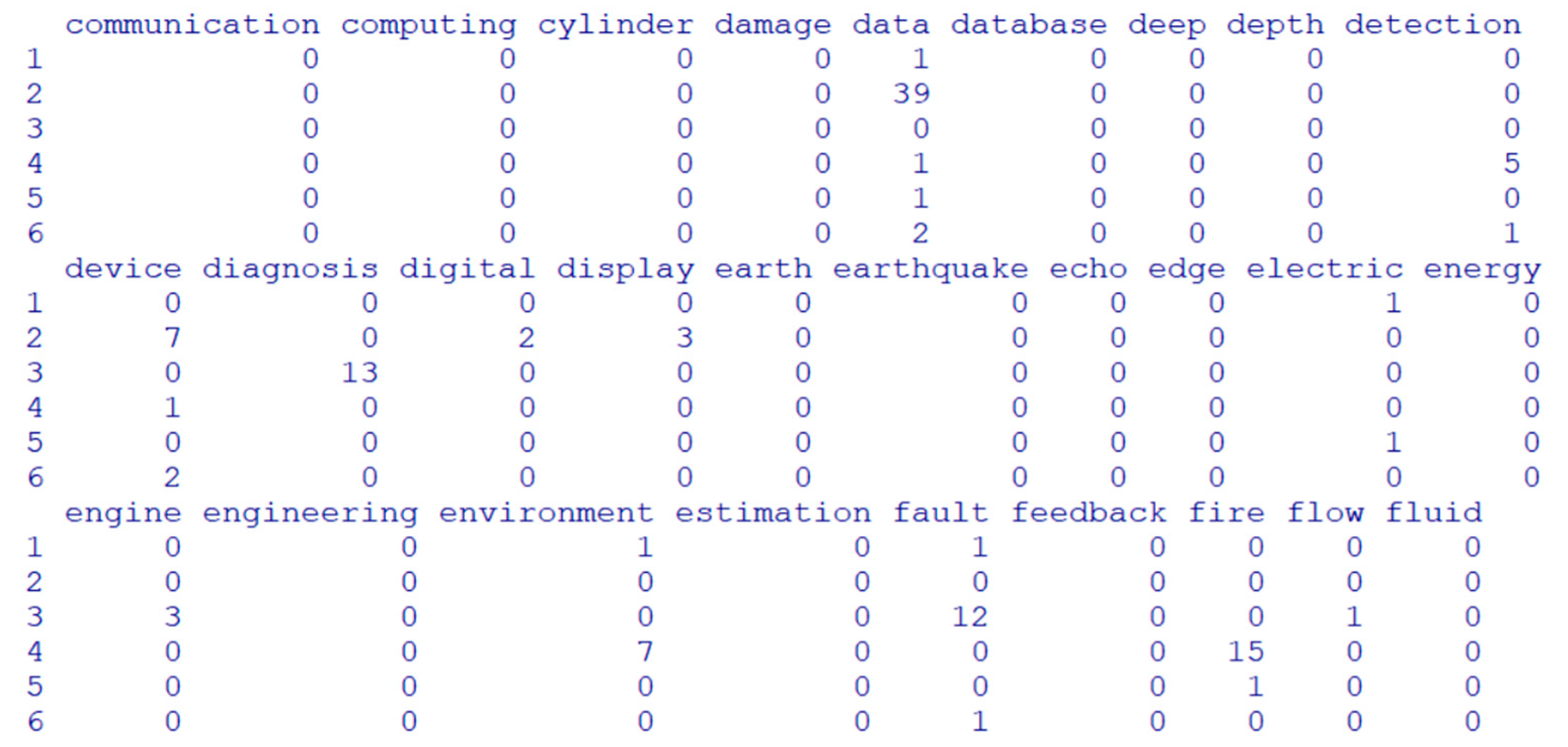
Keyword data analysis has been actively performed in various big data fields [1,2,3]. This is because a significant portion of big data consists of text-based data. To carry out a text data analysis, we preprocess the text data, such as a document, and extract the keywords from the preprocessed text data by text mining techniques [4,5]. In general, we construct a document–keyword matrix, with documents and keywords corresponding to its rows and columns [1,5,6,7]. Each element of the matrix is the frequency value of a keyword occurring in a document. Figure 1 shows a document–keyword matrix [7].
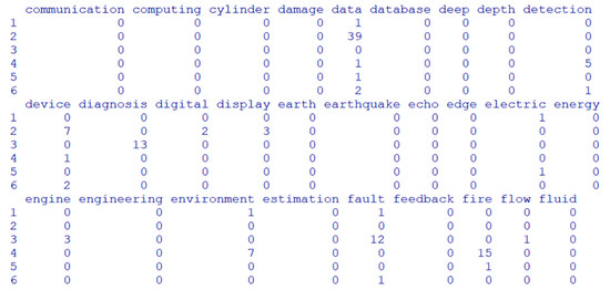
Figure 1.
A document–keyword matrix.
Even if a large amount of text big data is collected, the size of the data set is reduced through preprocessing to build structured data which can be analyzed by statistics and machine learning. Additionally, as can be seen in Figure 1, the preprocessed text data contain many zero values because a keyword that is included only once among all documents is assigned to one column in the document–keyword data.
In the previous research attempting to overcome the zero-inflation problem in text data analysis, Uhm and Jun (2022) proposed a generative model based on statistics by synthpop to address the zero-inflation problem in patent data analysis [6]. Jun (2023) studied generative adversarial network (GAN) and statistical modeling [1]. He compared the performance of GAN with the statistical model without GAN. Park and Jun (2023) used compound Poisson models to perform zero-inflation patent data analysis [7]. This was not a generative model but an exponential dispersion model. In this paper, to solve the problems of zero inflation as well as data shortage, we propose a keyword data analysis using generative models based on statistics and machine learning. Using these generative models, we generate synthetic data from the original data, and add the synthetic data to the original training and test data sets for keyword data analysis by various machine learning algorithms such as deep learning, linear modeling, Bayesian neural networks, etc.
Our paper consists of the following sections. In Section 2, we outline the background to our research, such as keyword data analysis and generative modeling. We propose the generative models based on statistics and machine learning for keyword data analysis in Section 3. In the next section, we carry out the experiments using simulation and patent document data to show the performance results for the compared models. We explain the conclusions and contributions of our paper in the last section.
2. Research Background
2.1. Keyword Data Analysis
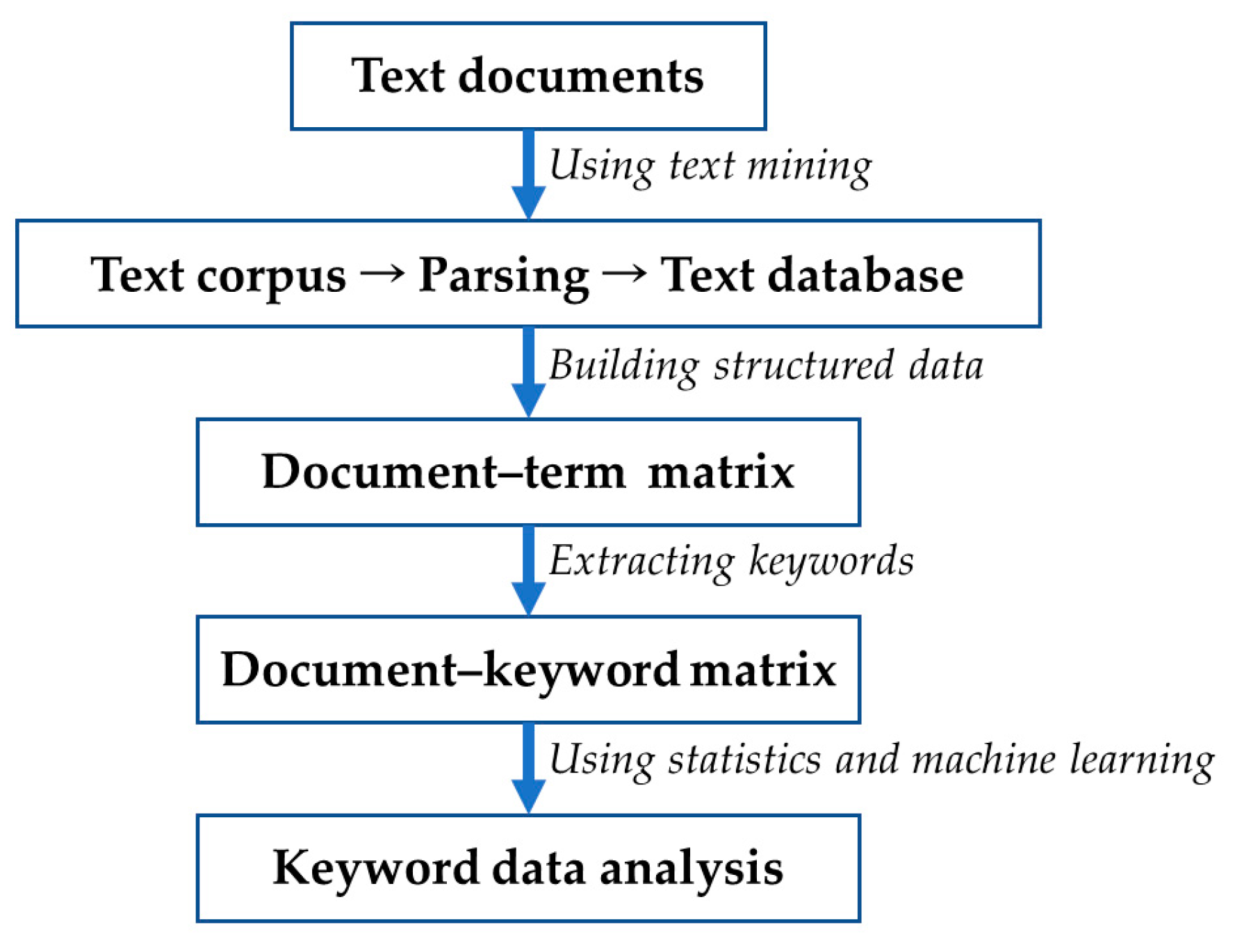
In this paper, we employ keyword data analysis to find the relationship between the keywords extracted from various text documents. Generally, we can extract the keywords from documents using term frequency (tf), inverse document frequency (idf) and domain experts’ knowledge and analyze them [4,5]. Figure 2 shows the process of keyword data analysis [4,5].
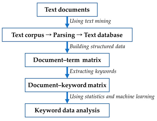
Figure 2.
Process of keyword data analysis.
In the process of keyword data analysis, we first collect text documents to be analyzed. Using text mining techniques, we create a text corpus, carry out parsing and construct a text database [5]. Next, we build a document–term matrix to serve as structured data for statistical analysis and machine learning. Finally, we extract keywords from the document–term matrix for keyword data analysis. In general, the data size of the document–keyword matrix constructed from collected text documents is reduced as it goes through preprocessing for text mining. Therefore, we need new methods to solve the data shortage problem. In this paper, we study the use of generative models to increase the data size of a document–keyword matrix.
2.2. Generative Modeling
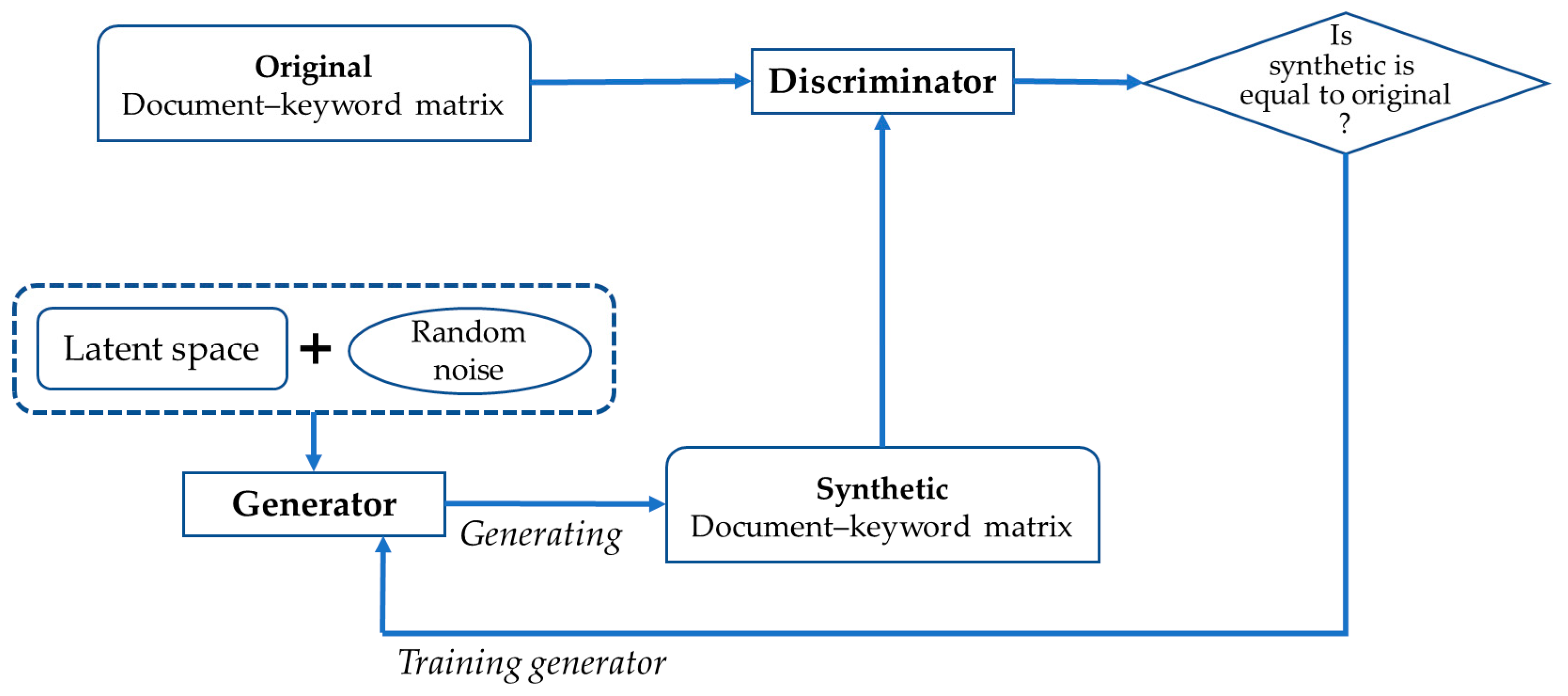
A generative model is a probabilistic and machine learning model to generate synthetic data that resemble given original data [8,9,10]. Figure 3 illustrate the process of generative modeling [8].

Figure 3.
Generative modeling.
By learning from the original data, we can construct generative models. To generate the synthetic data, we sample new data from the generative models with random noise [11]. The generative models use a probability distribution such as normal with mean () and variance () [12,13]. That is, the generative models are not deterministic and they generate different data every time. Therefore, we have to estimate the parameters of the probability distribution to explain the original data well. In the generative modeling, we estimate the density of the observed data () [14,15]. Currently, various studies are being actively conducted on generative models based on statistics and machine learning [16,17,18,19,20,21,22]. In the field of biology, single-cell genomic data also take the form of large count matrices characterized by a high occurrence of zeros. This presents the same issue as zero inflation in our study. Therefore, various tailored analysis methods have been investigated to address the unique challenges posed by such data [23,24]. The following two studies focus on generative models to solve the zero-inflation problem that arises in the analysis of single-cell genomic data. The first, by Liu et al. (2021), introduced one of the most widely adopted approaches to this problem [24]. The second, by Ji et al. (2023), detailed a method that employs a generative model in the single-cell genomic data analysis [23]. These references serve as a valuable entry point for extensive research on the analysis of single-cell genomic data using generative models. Most studies on generative models focus on image data, but in this study, we deal with generative models for count data because the document–keyword matrix consists of the frequency values of keywords occurring in documents.
2.3. Zero-Inflation Problems in Keyword Data Analysis
For keyword data analysis, we construct the document–keyword matrix according to the process of keyword data analysis illustrated in Figure 2. As we explained in Figure 1, there is a zero-inflation problem in the matrix. Many previous works have been conducted to solve the problem. Most of them were based on statistical methods. The zero-inflated count model is a popular method to analyze keyword data with zero inflation. This is defined as follows [25]:
where is the probability of zero. In Equation (1), the zero-inflated model consists of two components, zero and non-zero parts. Also, is a base model of probability mass function (pmf). In the zero-inflated count model, we use Poisson and negative binomial distributions for the pmf, and we call them zero-inflated Poisson (ZIP) and zero-inflated negative binomial (ZINB) models [26]. To improve the models based on ZIP and ZINB, Bayesian inference has been applied to the zero-inflated count model [27,28]. Neelon and Chung (2017) used the Bayesian latent factor model for the ZIP, and called this LZIP. They compared the LZIP with ZIP, and verified the improved performance of LZIP in the illustrative examples [27]. Moriña et al. (2021) proposed a method to analyze zero-inflated binomial data using Bayesian inference [28]. Seo and Hwang (2022) studied a Bayesian inference for ZINB regression model [29]. Another approach to overcome the zero-inflation problem is methods based on machine learning, such as classification and regression trees or generative models [1,6]. In this paper, we conduct research on generative models based on statistics and machine learning algorithms to solve the zero-inflation problem that occurs during keyword data analysis. Also, in our experiments, we compare the performance between models with synthetic data generation using the generative models based on statistical methods and machine learning algorithms.
3. Proposed Method
Much big data is in text form. Therefore, we have to extract the keywords from text data and analyze them by methods such as constructing document–keyword matrices, N-grams and correlation analysis between keywords, sentiment analysis, topic modeling, etc. [4,5]. The first task to be performed in keyword data analysis is to collect text documents on a given topic. As explained in Figure 2, the collected document data are preprocessed using text mining and natural language processing techniques. The preprocessed text document data set has a frequency matrix structure in which the rows and columns are documents and terms, respectively, as shown in Figure 1. This matrix is called the document–term matrix [5]. Next, we extract the keywords from the document–term matrix and construct the document–keyword matrix, as shown in Table 1.

Table 1.
Document–keyword matrix and frequency element.
In Table 1, the Frequencyij is the frequency value of Keywordj occurring in Documenti. Through the data preprocessing, the size of the initially collected document data set gradually decreases, and when the document–keyword matrix is finally constructed, the data set sometimes becomes so small that it is difficult to analyze. In addition, many elements of the matrix are zero values, as shown in Figure 1. Not only the data shortage but also the zero-inflation problem must be solved in keyword data analysis [1,6,7,25,26,28,30]. To solve these problems, we use generative models based on statistics and machine learning. First, we consider the synthpop package of R data language to generate synthetic data [31,32]. This is a generative model based on statistics. In the synthpop modeling, the original input data are represented as follows.
In the data of (2), is the number of input variables. The synthpop model uses classification and regression trees (CART) to generate the synthetic data [16,31]. We generate the synthetic data for the current variable using the previous variables as follows: We start with the second variable and exclude the first variable [31]. We generate by running using CART growth. That is, we sample from the CART model, [16]. Figure 4 explains the method of synthetic data generation by the synthpop in our keyword data analysis.
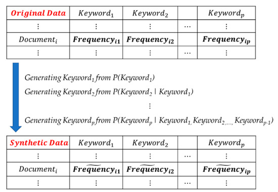
Figure 4.
Generating a synthetic document–keyword matrix using synthpop.
In Figure 4, we fit statistical models of the keywords to the original data and generate synthetic data that is completely new data of the keywords. We denote original and synthetic data as and . Using the original data, we find the joint probability distribution of keywords. We represent the probability distribution of as Equation (3).
In Equation (3), we generate the from the conditional probability distribution of given . The synthpop begins by estimating the probability distribution of the first keyword, . Next, we generate new data (synthetic) that resembles (original) by . That is, the synthetic data represent the original data . Using this result, we build the conditional distribution and generate the synthetic data for by the conditional distribution. In this way, we generate the final synthetic data .
Unlike the synthpop, the generative model based on machine learning is performed by deep neural networks [9,33]. In this paper, we use GAN for the generative model for document–keyword data generation. GAN is a machine learning model which generates new synthetic data that resemble the given original data [9,11,12,13,17]. GAN performs an adversarial training process, involving two neural networks, a generator and discriminator. The formula of GAN is defined as follows [9].
where and represent the generator and discriminator respectively. and are input data and random noise, which follow a normal distribution. In Equation (4), also is the latent representation of . and are the generative and latent models. The discriminator wants to maximize , and on the other side, the generator tries to minimize . In this paper, the document–keyword matrix is used as in Equation (4). Figure 5 illustrates the process of generating a synthetic document–keyword matrix using GAN.
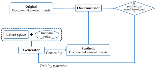
Figure 5.
Generating synthetic document–keyword matrix using GAN.
In Figure 5, the generator creates a new synthetic document–keyword matrix from latent space and random noise. Also, the generator tries to make the synthetic data as similar as possible to the original data. The latent space is a learning space representing sample data with low dimension. Sample data that are similar to each other are located close to each other in the latent space. We select the initial data point from the latent space and add random noise to the data. Thus, we generate the synthetic document–keyword matrix from the latent space and random noise. The discriminator predicts whether the input data are real (original) or fake (not original). Sampling the document–keyword data randomly from original and synthetic data sets, and combining the sample data, the discriminator uses this data to learn to accurately classify real and fake. The generator is trained so that the discriminator can judge the synthetic data as original. Ultimately, the generator aims to generate synthetic data to the extent that the discriminator cannot distinguish whether the synthetic data are original or not. When training the entire model, only the weights of generator should be updated and the weights of discriminator should not be updated so that the synthetic data with good performance are generated. Next, we combine the results of synthpop and GAN. Figure 6 shows the synthetic data generation.

Figure 6.
Generating synthetic document–keyword matrix using synthpop and GAN.
Our third generative model combines the two data sets generated by synthpop and GAN. In Figure 6, synthpop and GAN generate synthetic document–keyword data sets based on statistics and machine learning, respectively. Therefore, we use the three generative models to analyze the keyword data. In our keyword data analysis, we build the linear model shown in Equation (5).
where are k explanatory keywords and is a response keyword. Each variable of (5) represents the frequency value of a keyword. To evaluate the performance between generative models, in this paper, we divide the given data into training (70%) and test (30%) data sets. Using the training data, we calculate the Akaike information criterion (AIC) and use this value to compare the explanatory power of the linear model [34]. AIC is a measure used in predictive modeling to verify the goodness of fit of a model, as shown in Equation (6) [35,36].
where and represent the model parameter and data, respectively. is the number of model parameters. is maximum likelihood estimator of . The better the fitting performance of model, the smaller the AIC value. We use another measure, mean squared error (MSE), to evaluate performance of the compared models. MSE is defined as shown in Equation (7) [34,35,36,37].
where and are real and predicted values, respectively, and is the size of the given data. We calculate MSE value of each model using the test data. The smaller the MSE value of the model, the better its predictive performance. In the next section, we perform a performance comparison between the compared generative models using MSE and AIC.
4. Experimental Results
4.1. Simulation Data Analysis
In keyword data analysis, each element of a document–keyword matrix is the frequency value of keyword occurring in document. This count data follows a Poisson distribution [7,38]. Thus, we generated the random numbers from the multivariate generalized Poisson distribution [39,40]. We used the R data language and R package for generating simulation data and data analysis [32,40]. For our simulation data for keyword data analysis, we considered the mixture of Poisson distributions with two parameters, rate and dispersion [39,40,41]. In our simulation study, we consider a linear model with six variables (keywords), as shown in Equation (8).
where is the response keyword and () are explanatory keywords. Each keyword in () follows a Poisson distribution with different parameters. Also, they are correlated with each other. Figure 7 shows the correlation structure of the generated simulation data.

Figure 7.
Correlation matrix of a simulation data set.
In Figure 7, we can see that among the explanatory variables, some variables have a high correlation with the response variable Y, while others have a relatively low correlation. Also, in Table 2, we illustrate the zero ratio of each variable in the simulation data.

Table 2.
Zero ratio of each variable in a simulation data set.
We can see that the percentage of zeros in X2 and X4 is more than 50%. In this way, we created simulation data so that the zero-inflation problem could be included in the original data. Next, we utilized the generative models to create synthetic data and analyze them based on the linear model in (7). In addition, we calculated the AIC and MSE values of the constructed models using original and synthetic data sets. We show the AIC values of the compared models in Table 3.

Table 3.
AIC values of compared models: simulation data.
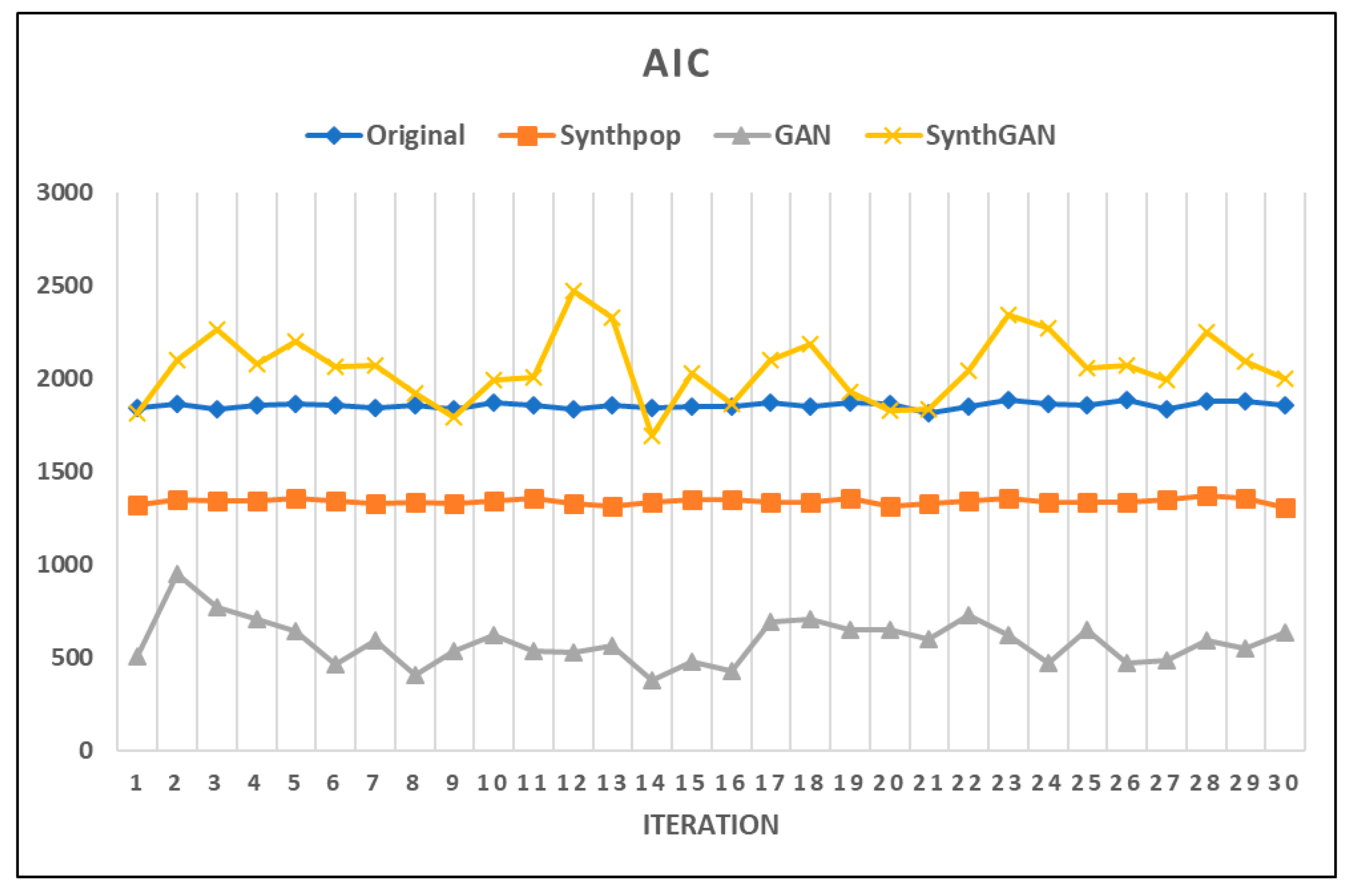
In Table 3, We built the linear model in Equation (7) for the four data sets and calculated the AIC value for each model. The elements of original data are count data because they were generated from a generalized Poisson distribution. The synthetic data generated by synthpop from the original data are also count data because they are created by a joint distribution of frequency count data. However, the synthetic data set created by GAN is a continuous data type because the generator of GAN creates the new data from the latent space of a normal distribution and random noise. In this paper, it is possible to use continuous data because the constructed linear model of keywords allows such data. Lastly, we combined the synthetic data sets from synthpop and GAN (SynthGAN). Figure 8 is a visualization of the AIC values in Table 3.
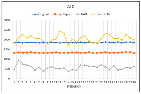
Figure 8.
AIC plot of compared models.
The AIC values of the GAN synthetic data are the smallest. The values for the synthpop synthetic data are also smaller than the original data, but the AIC values for synthGAN are mostly larger than the original data. Therefore, from the perspective of model fitting, we were able to confirm the validity of using the synthetic data by synthpop and GAN. Although the AIC values of the GAN synthetic data are smaller than those of synthpop, the dispersion of the AIC values is larger than for the original. Also, in Figure 8, we can see that there is a large variation in the AIC values of the models based on GAN. This is because random noise was used in the synthetic data generation process using the GAN model, thereby increasing the variance in the data. Next, we present the MSE results of models for the comparative data sets in Table 4.

Table 4.
MSE values of compared models: simulation data.
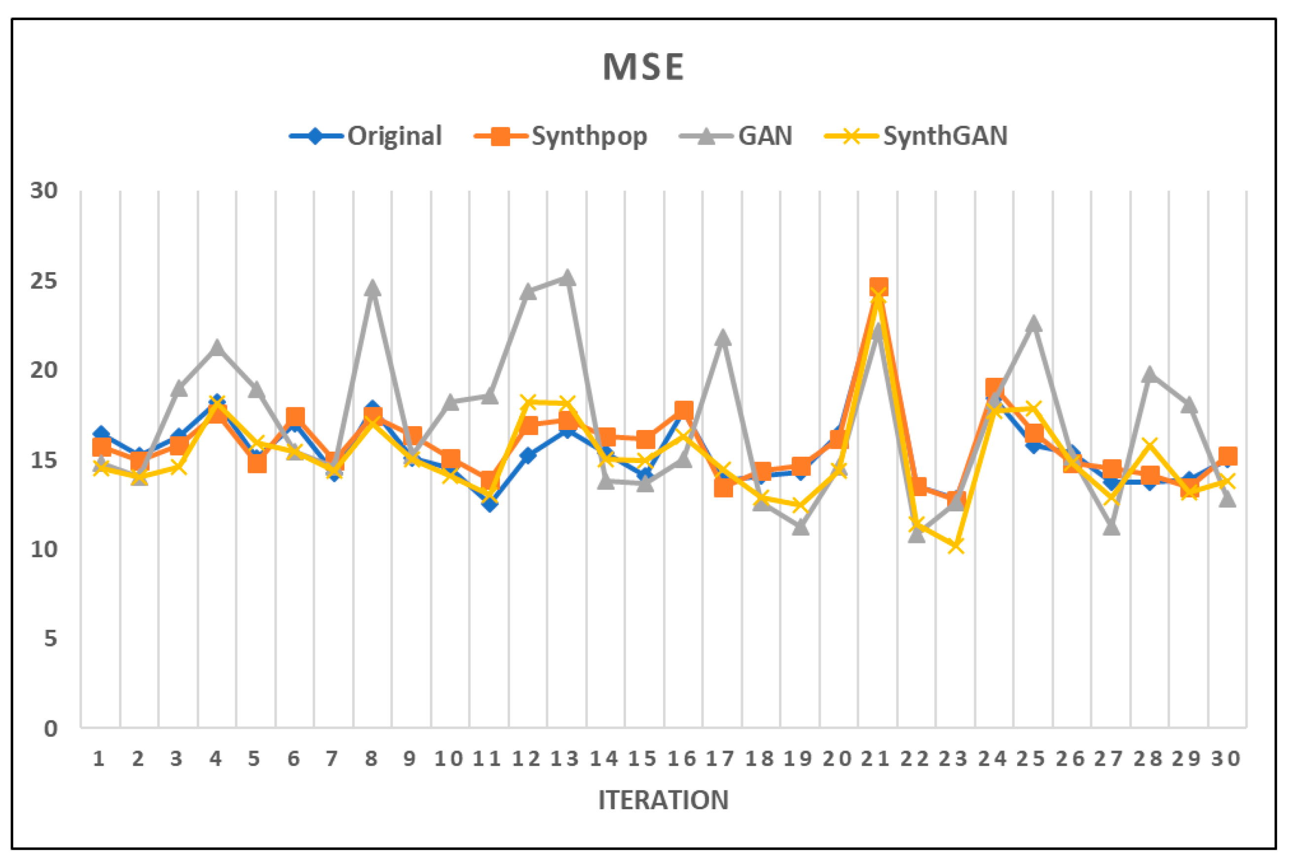
By comparing the MSE values of the models, we can check the prediction performance between the compared models. We confirmed in Table 4 that the difference in MSE values for the compared models was not large. Figure 9 shows the MSE plot of compared models with the original and synthetic data sets.
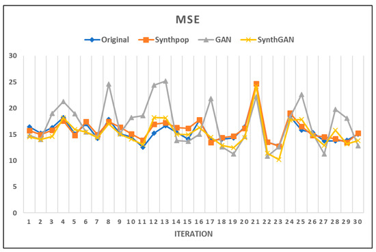
Figure 9.
MSE plot of compared models.
In many repeated experiments, we confirmed that the MSE values for the GAN synthetic data were calculated to be larger than those for the remaining three comparison data sets in Figure 9. Therefore, in terms of the predictive performance, the use of synthetic data by synthpop is not significantly different from the original data. Thus, we confirmed the validity of using the synthetic data by synthpop. In addition, we can see that the MSE values of the GAN model are distributed over a wide range. Similar to the results in Figure 8, this is because we use random noise from the latent space when we generate reproduction data using the GAN model. Table 5 shows a summary of the MSE values of the original and synthetic data sets.

Table 5.
Summary of MSE values.
In Table 5, Q1 and Q3 are the percentiles of 25% and 75%, respectively. The mean value of the synthetic data from GAN is the largest among the compared models. Also, the minimum value in the GAN synthetic data is smaller than that of the original and synthpop data, and the maximum value in the GAN data is larger than those of the other data sets. Therefore, we can see that the performance of the GAN synthetic data was poor compared with the other models and that the dispersion of GAN synthetic data was large. Therefore, considering the results of simulation data analysis, although the AIC values of the synthetic data generated by GAN are small compared with those of the other data sets, the MSE values are large and their dispersion is also large. We found that synthpop synthetic data is the most appropriate for the linear prediction model for keyword data analysis.
4.2. Practical Data Analysis
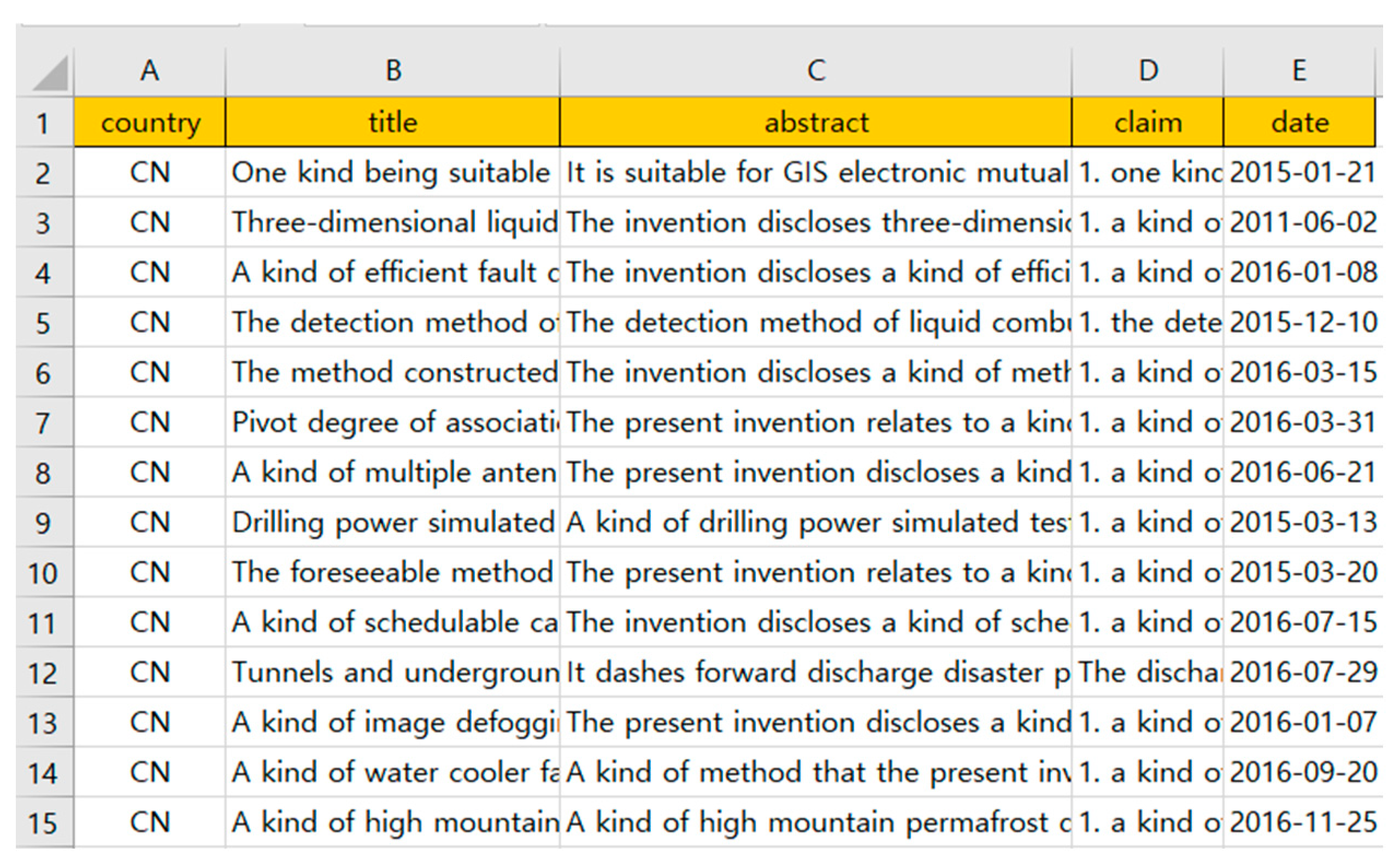
To show how the proposed research can be applied to a practical domain, we used the patent document data related to artificial intelligence (AI) technology for disaster and security for text data. We searched the patent documents from the United States Patent and Trademark Office and the Korea Intellectual Property Rights Information Service [42,43]. The collected patent documents were filed until 2022 in patent databases around the world. We obtained a total of 16,875 valid patents through the patent verification process. Figure 10 shows the valid patent data.
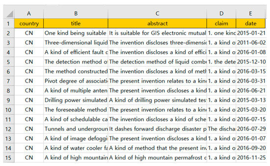
Figure 10.
Valid patent documents.
In this experiment, we selected the title and abstract from the patent data in Figure 10 for keyword data analysis. Using text mining techniques, we constructed the document–keyword matrix from the valid patent documents, as shown in Figure 11.
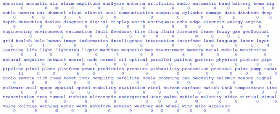
Figure 11.
Our document–keyword matrix of AI patents.
Figure 11 shows the first rows of 162 keywords in a document–keyword matrix. We carried out a 10% sampling from the matrix with 16,875 rows (documents). To compare the performance between the original and synthetic data sets, we used a linear model, as shown in Equation (9).
We selected Analysis for the response keyword, and Data, Image, Information, Signal and Time for the explanatory keywords. We show the AIC values of the compared models in Table 6.

Table 6.
AIC values of compared models: patent data.
In Table 6, as for the results of the simulation data, the AIC values of the synthetic data by GAN are the smallest in all data sets, both original and synthetic. In addition, the AIC values of the original and synthpop synthetic data are similar to each other. The AIC values of synthetic data by synthGAN are larger than the original and synthpop values. Therefore, we confirmed that synthpop synthetic data can well replace original data. Next, we calculated the MSE values of the compared models. We show the experimental results in Table 7.

Table 7.
MSE values of compared models: patent data.
Similar to the experimental results using simulated data, we found that the GAN synthetic data had the largest MSE values in the comparison using practical patent data. Also, the MSE dispersion of the GAN synthetic data is larger than that of the others. In comparison to this, the MSE values of the synthpop synthetic data are similar to the results of the original data. We were able to see that the MSE results for synthGAN were also similar to the results for the original and synthpop data. Therefore, we confirmed that the synthpop generative model is the most efficient way to perform synthetic data generation for keyword data analysis.
5. Discussion
In this paper, we tried to solve the zero-inflation problem that occurs in the process of keyword data analysis. We carried out two experiments using simulation and practical models. From the experimental results, we found that the performances of the synthpop and GAN models were better than the original model. This means that using the generative models based on statistics and machine learning is better than not using them. Also, the performance of the GAN model was better than that of synthpop. For example, all the AIC values of GAN were smaller than the values of the synthpop model in the simulation data analysis of Figure 8. This was similar to the results for AIC values when comparing models in the practical data analysis of Table 6. The GAN model has the best performance due to its characteristics as a generative model. When we generate the synthetic data using the GAN model, we generally perform random sampling from a normal distribution representing the latent space. Thus, most of the generated data values are distributed around the mean. Because the variance of the synthetic data generated by GAN is relatively small compared with other generative models, the performance of the compared linear model is stable and shows excellent explanatory power.
Currently, generative models are actively used in various machine learning domains. In this study, we used this model to solve the zero-inflation problem that occurs during the analysis of keyword data extracted from text documents. Of course, generative models show excellent performance in the image data field, but we showed the utility and improved performance of generative models in the field of numerical data including zero. We generated synthetic data from the generative models and analyzed them by statistical methods such as linear regression. Finally, we overcame the zero-inflation problem using the generative models for keyword data analysis. We expect that our research will be used more broadly to solve data sparsity problems, including the zero-inflation problem. Finally, we found that using simulation data to evaluate the performance of generative models can lead to over-optimistic conclusions. Therefore, we decided that experiments using more diverse practical data would be necessary to efficiently evaluate the performance of the generative model.
6. Conclusions
The aim of our study is to generate synthetic data and analyze it for prediction. Most studies related to generative models are interested in the generative model itself that creates synthetic data, but our focus is on constructing a predictive model by analyzing data sampled from the constructed generative models. For this reason, AIC and MSE were used to evaluate the performance of the model in this paper. Thus, we generated and analyzed more synthetic data. In the process of keyword data analysis, we face the problems of a lack of data and zero inflation. These problems become factors that degrade the performance of machine learning models for keyword data analysis. To solve these problems, we proposed the use of generative models. We considered generative models based on statistics and machine learning, such as synthpop, GAN and synthGAN, in this paper. Also, we compared the model performance between the original and synthetic data sets using the measures of AIC and MSE. From the experimental results using simulation data and practical patent documents, we verified the better performance of generative modeling by synthpop compared with the other models. We also found that the AIC values of the GAN synthetic data were the smallest among the compared models. However, its MSE values were not the smallest but the largest. Due to these results, we confirmed the difficulty in analyzing keyword data using the synthetic data by GAN.
In this paper, we conclude that the synthpop generative model is the best method to generate synthetic data for keyword data analysis. Of course, the generative model using GAN is also an excellent model from the AIC perspective, but its performance is poor from the MSE perspective. Therefore, in our future works, we will study new methods to improve the MSE of GAN synthetic data for keyword data analysis. We will add Bayesian learning or various probability distributions to traditional GAN to improve the performance of generative models using GAN in keyword data analysis. Our research contributes a method for creating new synthetic data in text big data analysis. This is necessary because the data size is reduced during the preprocessing of text data. In particular, a sufficient amount of data is required to perform large-scale machine learning such as deep learning. Therefore, synthetic data from generative models will contribute to solving the lack of original data to perform machine learning.
Funding
This research received no external funding.
Data Availability Statement
The data presented in this study are available on request from the corresponding author (status: privacy).
Conflicts of Interest
The author declares no conflicts of interest.
References
- Jun, S. Zero-Inflated Text Data Analysis using Generative Adversarial Networks and Statistical Modeling. Computers 2023, 12, 258. [Google Scholar] [CrossRef]
- Shin, H.; Lee, H.J.; Cho, S. General-use unsupervised keyword extraction model for keyword analysis. Expert Syst. Appl. 2023, 233, 120889. [Google Scholar] [CrossRef]
- Bzhalava, L.; Kaivo-oja, J.; Hassan, S.S. Digital business foresight: Keyword-based analysis and CorEx topic modeling. Futures 2024, 155, 103303. [Google Scholar] [CrossRef]
- Julia, S.; Robinson, D. Text Mining with R; O’Reilly: Sebastopol, CA, USA, 2017. [Google Scholar]
- Feinerer, I.; Hornik, K. Package ‘tm’ Version 0.7-11, Text Mining Package; CRAN of R Project, R Foundation for Statistical Computing: Vienna, Austria, 2023. [Google Scholar]
- Uhm, D.; Jun, S. Zero-Inflated Patent Data Analysis Using Generating Synthetic Samples. Future Internet 2022, 14, 211. [Google Scholar] [CrossRef]
- Park, S.; Jun, S. Zero-Inflated Patent Data Analysis Using Compound Poisson Models. Appl. Sci. 2023, 13, 4505. [Google Scholar] [CrossRef]
- Foster, D.; Friston, K. Generative Deep Learning: Teaching Machines to Paint, Write, Compose, and Play, 2nd ed.; O’REILLY: Sebastopol, CA, USA, 2023. [Google Scholar]
- Goodfellow, I.; Pouget-Abadie, J.; Mirza, M.; Xu, B.; Warde-Farley, D.; Ozair, S.; Courville, A.; Bengio, Y. Generative Adversarial Nets. In Proceedings of the 27th International Conference on Neural Information Processing Systems, Montreal, QC, Canada, 8–13 December 2014; pp. 1–9. [Google Scholar]
- Bau, D.; Liu, S.; Wang, T.; Zhu, J.Y.; Torralba, A. Rewriting a deep generative model. In Proceedings of the 16th European Conference on Computer Vision–ECCV, Glasgow, UK, 23–28 August 2020; pp. 351–369. [Google Scholar]
- Deng, L.; He, C.; Xu, G.; Zhu, H.; Wang, H. PcGAN: A Noise Robust Conditional Generative Adversarial Network for One Shot Learning. IEEE Trans. Intell. Transp. Syst. 2022, 23, 25249–25258. [Google Scholar] [CrossRef]
- Li, C.; Xu, K.; Zhu, J.; Liu, J.; Zhang, B. Triple Generative Adversarial Networks. IEEE Trans. Pattern Anal. Mach. Intell. 2022, 44, 9629–9640. [Google Scholar] [CrossRef] [PubMed]
- Rosenfeld, B.; Simeone, O.; Rajendran, B. Spiking Generative Adversarial Networks with a Neural Network Discriminator: Local Training, Bayesian Models, and Continual Meta-Learning. IEEE Trans. Comput. 2022, 71, 2778–2791. [Google Scholar] [CrossRef]
- Ruthotto, L.; Haber, E. An introduction to deep generative modeling. GAMM-Mitteilungen 2021, 44, e202100008. [Google Scholar] [CrossRef]
- Zhou, X.; Hu, Y.; Wu, J.; Liang, W.; Ma, J.; Jin, Q. Distribution Bias Aware Collaborative Generative Adversarial Network for Imbalanced Deep Learning in Industrial IoT. IEEE Trans. Ind. Inform. 2023, 19, 570–580. [Google Scholar] [CrossRef]
- Nowok, B.; Raab, G.M.; Dibben, C. synthpop: Bespoke Creation of Synthetic Data in R. J. Stat. Softw. 2016, 74, 1–26. [Google Scholar] [CrossRef]
- Xu, M.; Baraldi, P.; Lu, X.; Zio, E. Generative Adversarial Networks with AdaBoost Ensemble Learning for Anomaly Detection in High-Speed Train Automatic Doors. IEEE Trans. Intell. Transp. Syst. 2022, 23, 23408–23421. [Google Scholar] [CrossRef]
- Yan, C.; Chang, X.; Li, Z.; Guan, W.; Ge, Z.; Zhu, L.; Zheng, Q. ZeroNAS: Differentiable Generative Adversarial Networks Search for Zero-Shot Learning. IEEE Trans. Pattern Anal. Mach. Intell. 2022, 44, 9733–9740. [Google Scholar] [CrossRef]
- Tang, C.; He, Z.; Li, Y.; Lv, J. Zero-Shot Learning via Structure-Aligned Generative Adversarial Network. IEEE Trans. Neural Netw. Learn. Syst. 2022, 33, 6749–6762. [Google Scholar] [CrossRef] [PubMed]
- You, H.; Cheng, Y.; Cheng, T.; Li, C.; Zhou, P. Bayesian Cycle-Consistent Generative Adversarial Networks via Marginalizing Latent Sampling. IEEE Trans. Neural Netw. Learn. Syst. 2021, 32, 4389–4403. [Google Scholar] [CrossRef] [PubMed]
- Li, H.; Prasad, R.G.N.; Sekuboyina, A.; Niu, C.; Bai, S.; Hemmert, W.; Menze, B. Micro-Ct Synthesis and Inner Ear Super Resolution via Generative Adversarial Networks and Bayesian Inference. In Proceedings of the IEEE 18th International Symposium on Biomedical Imaging (ISBI), Nice, France, 13–16 April 2021; pp. 1500–1504. [Google Scholar]
- Yan, R.; Yuan, Y.; Wang, Z.; Geng, G.; Jiang, Q. Active Distribution System Synthesis via Unbalanced Graph Generative Adversarial Network. IEEE Trans. Power Syst. 2022, 38, 4293–4307. [Google Scholar] [CrossRef]
- Ji, X.; Tsao, D.; Bai, K.; Tsao, M.; Xing, L.; Zhang, X. scAnnotate: An automated cell-type annotation tool for single-cell RNA-sequencing data. Bioinform. Adv. 2023, 3, vbad030. [Google Scholar] [CrossRef] [PubMed]
- Liu, Q.; Chen, S.; Jiang, R.; Wong, W.H. Simultaneous deep generative modelling and clustering of single-cell genomic data. Nat. Mach. Intell. 2021, 3, 536–544. [Google Scholar] [CrossRef]
- Cameron, A.C.; Trivedi, P.K. Regression Analysis of Count Data, 2nd ed.; Cambridge University Press: New York, NY, USA, 2013. [Google Scholar]
- Hilbe, J.M. Modeling Count Data; Cambridge University Press: New York, NY, USA, 2014. [Google Scholar]
- Neelon, B.; Chung, D. The LZIP: A Bayesian Latent Factor Model for Correlated Zero-Inflated Counts. Biometrics 2017, 73, 185–196. [Google Scholar] [CrossRef] [PubMed]
- Moriña, D.; Puig, P.; Navarro, A. Analysis of zero inflated dichotomous variables from a Bayesian perspective: Application to occupational health. BMC Med. Res. Methodol. 2021, 21, 277. [Google Scholar] [CrossRef]
- Seo, G.T.; Hwang, B.S. A Bayesian zero-inflated negative binomial regression model based on Pólya-Gamma latent variables with an application to pharmaceutical data. Korean J. Appl. Stat. 2022, 35, 311–325. [Google Scholar]
- Sidumo, B.; Sonono, E.; Takaidza, I. Count Regression and Machine Learning Techniques for Zero-Inflated Overdispersed Count Data: Application to Ecological Data. Ann. Data Sci. 2023. [Google Scholar] [CrossRef]
- Nowok, B.; Raab, G.M.; Snoke, J.; Dibben, C.; Nowok, M.B. Package ‘synthpop’ Ver. 1.8–0, Generating Synthetic Versions of Sensitive Microdata for Statistical Disclosure Control; CRAN of R Project, R Foundation for Statistical Computing: Vienna, Austria, 2022. [Google Scholar]
- R Development Core Team. R: A Language and Environment for Statistical Computing; R Foundation for Statistical Computing: Vienna, Austria; Available online: http://www.R-project.org (accessed on 1 October 2023).
- Neunhoeffer, M. Package ‘RGAN’ Version 0.1.1, Generative Adversarial Nets (GAN) in R; CRAN of R Project, R Foundation for Statistical Computing: Vienna, Austria, 2022. [Google Scholar]
- Montgomery, D.C.; Peck, E.A.; Vining, G.G. Introduction to Linear Regression Analysis; John Wiley & Sons: Hoboken, NJ, USA, 2012. [Google Scholar]
- Murphy, K.P. Machine Learning: A Probabilistic Perspective; MIT Press: Cambridge, MA, USA, 2012. [Google Scholar]
- Theodoridis, S. Machine Learning A Bayesian and Optimization Perspective; Elsevier: London, UK, 2015. [Google Scholar]
- Bruce, P.; Bruce, A.; Gedeck, P. Practical Statistics for Data Scientists; O’Reilly Media: Sebastopol, CA, USA, 2020. [Google Scholar]
- Makowski, M.; Piotrowski, E.W. Transactional Interpretation and the Generalized Poisson Distribution. Entropy 2022, 24, 1416. [Google Scholar] [CrossRef] [PubMed]
- Li, H.; Demirtas, H.; Chen, R. RNGforGPD An R Package for Generation of Univariate and Multivariate Generalized Poisson Data. R J. 2020, 12, 173–188. [Google Scholar] [CrossRef]
- Li, H.; Chen, R.; Nguyen, H.; Chung, Y.; Gao, R.; Demirtas, H. Package ‘RNGforGPD’ Version 1.1.0, Random Number Generation for Generalized Poisson Distribution; CRAN of R Project, R Foundation for Statistical Computing: Vienna, Austria, 2022. [Google Scholar]
- Li, X.-J.; Tian, G.-L.; Zhang, M.; Ho, G.T.S.; Li, S. Modeling Under-Dispersed Count Data by the Generalized Poisson Distribution via Two New MM Algorithms. Mathematics 2023, 11, 1478. [Google Scholar] [CrossRef]
- USPTO. The United States Patent and Trademark Office. Available online: http://www.uspto.gov (accessed on 1 October 2023).
- KIPRIS. Korea Intellectual Property Rights Information Service. Available online: www.kipris.or.kr (accessed on 1 October 2023).
Disclaimer/Publisher’s Note: The statements, opinions and data contained in all publications are solely those of the individual author(s) and contributor(s) and not of MDPI and/or the editor(s). MDPI and/or the editor(s) disclaim responsibility for any injury to people or property resulting from any ideas, methods, instructions or products referred to in the content. |
© 2024 by the author. Licensee MDPI, Basel, Switzerland. This article is an open access article distributed under the terms and conditions of the Creative Commons Attribution (CC BY) license (https://creativecommons.org/licenses/by/4.0/).

