Abstract
The aim of this work, which is an extension of previous research, is a comparative analysis of the results of the dynamic optimization of safe multi-object control, with different representations of the constraints of process state variables. These constraints are generated with an artificial neural network and take movable shapes in the form of a parabola, ellipse, hexagon, and circle. The developed algorithm allows one to determine a safe and optimal trajectory of an object when passing other multi-objects. The obtained results of the simulation tests of the algorithm allow for the selection of the best representation of the motion of passing objects in the form of neural constraints. Moreover, the obtained characteristics of the sensitivity of the object’s trajectory to the inaccuracy of the input data make it possible to select the best representation of the motion of other objects in the form of an excessive approximation area as neural constraints of the control process.
1. Introduction
Synthesizing the optimal control of single- and multi-object dynamic control processes is becoming an increasingly common challenge in practice. This applies to both non-autonomous and autonomous objects such as ships, cars, planes, and drones. One of many dynamic optimization methods can be used to solve this task.
Considering the significant impact of time-varying constraints on the control process, dynamic programming that meets Bellman’s optimality principle is the most effective optimization method, as presented in [1].
This research’s motivation was to expand the applications of the dynamic programming method to the synthesis of multi-object process control supported by artificial intelligence.
1.1. State of Knowledge
The scope of the literature presenting dynamic programming is wide, including software for solving dynamic programming tasks and applications in robotics, autonomous vehicles (AVs), unmanned air vehicles (UAVs), autonomous underwater vehicles (AUVs), and maritime autonomous surface ships (MASSs).
Regarding software for solving various practical dynamic programming tasks, we should first mention a tool called DynaProg developed by Miretti et al. and presented in [2]. It enables the optimization of deterministic, multi-stage, non-linear dynamic decision-making processes. In turn, in [3], Sundstrom et al. synthesized optimal control using dynamic programming in MATLAB version 2023 software. Knowledge of the control objective function and state equations of the control process with several state variables is required. Mikołajczak and Rumbut in [4] solved the problem of dynamic programming in a distributed artificial intelligence environment in C++ version 2023 software. Search management in a distributed development environment is optimized using Actors and Petri nets. Luus, in one of the chapters of the optimization encyclopedia [5], describes an iterative dynamic programming algorithm with variable stage lengths. An example of solving one of the very important optimization tasks using approximate dynamic programming is maximizing the number of survivors in a maritime disaster, as presented by Rempel et al. in [6], where the finite-horizon Markov decision process is used to describe the control process. Another category is the application of dynamic programming to solving the task of optimizing the course of a two-player game, which was presented by Gong et al. in [7]. The control objective function is the cost of capturing the target and has a linear–quadratic form.
Regarding the use of dynamic programming in robot design, the optimal control of tracking a robot manipulator with three degrees of freedom presented by Szuster and Gierlak in [8] using the dynamic programming method should be mentioned. The Lyapunov stability method is used to evaluate the optimization, and an artificial neural network is used to identify critical conditions. Then, the same authors in [9] presented the use of dual heuristic dynamic programming to solve the task of the optimal tracking control of an articulated robot manipulator. The duality of the control algorithm results from the two structures of the actor’s and the critic’s neural networks.
Many works have significantly contributed to the optimization of autonomous vehicle (AV) facilities. In [10], Kang and Jung presented the problem of identifying vehicle lanes using local line extraction and dynamic programming. The functional deviation of the actual vehicle movement line from the virtual straight line is minimized. In [11], Sundstrom et al. used dynamic programming to solve the problem of the optimal management of a hybrid vehicle’s electric energy. Thanks to this, a higher accuracy in achieving the global maximum was achieved. In [12], Silva and Sousa used dynamic programming to minimize a vehicle’s path deviation from a given path, considering uncertainties and environmental disturbances. In [13], Wei et al. presented the problem of optimizing the trajectories of many cars moving in a platoon formation, solved using dynamic and integer programming. In [14], Deshpande et al. solved the task of optimizing the energy consumption of connected and automated vehicles using dynamic programming. The process model was verified in real time. In [15], Lin et al. used dynamic programming to minimize the time needed for a group of vehicles to travel in a two-lane merging scenario. In [16], Wang et al. designed a real-time autonomous vehicle path-tracking controller using model-free adaptive dynamic programming. Compensation was made for non-linear external disturbances represented by an artificial neural network with a radial activation function. In [17], Lin et al. presented a programming algorithm for the dynamic planning and control of the path of an autonomous vehicle in situations of changing environments and surrounding vehicles.
Dynamic programming also has a large share in the optimization of unmanned air vehicles (UAVs). In [18], Gjorshevski et al. used a dynamic programming algorithm to determine the optimal trajectory in terms of the cost of the energy consumed by an unmanned aerial vehicle (UAV). Bouman et al. presented the use of dynamic programming to solve the traveling salesman problem with a drone in [19], using the example of optimizing product deliveries to customers using trucks and a drone. In [20], Flint and Fernandez solved the problem of planning the trajectories of many cooperating autonomous UAVs in the process of optimally searching an uncertain environment using dynamic programming. In [21], Azam et al. used a dynamic programming method to optimize the control of a swarm of UAVs, implementing the process of tracking the movement of multiple targets. Din et al. used dynamic programming in [22] to maximize the glide range performance of a UAV equipped with special actuating devices. In [23], Jennings et al. optimized the route planning of small unmanned aerial vehicles using dynamic programming, emphasizing the impact of wind disturbances.
Another area of application of dynamic programming is the optimization of various control tasks for autonomous underwater vehicles (AUVs). In [24], Vibhute used a dynamic programming method for the optimal motion control of an autonomous underwater vehicle (AUV), where the real-time identification of vehicle dynamics based on actuator input and obstacle position was used instead of a process model. In [25], Chen et al. used dynamic programming to optimally track the given trajectory of an autonomous underwater vehicle (AUV) using a fuzzy logic controller. In [26], Che and Hu solved the problem of the optimal tracking of an underactuated AUV’s trajectory using dynamic programming.
Dynamic programming is also used in synthesizing the optimal control of marine autonomous surface ships (MASSs). In [27], Wei and Zhou used dynamic programming to optimize the fuel consumption of a MASS along the weather route by controlling both the ship’s movement speed and heading changes. In [28], Geng et al. implemented an algorithm to plan the ship’s anti-collision route using dynamic programming using velocity obstacle models for stationary and moving targets. In [29], Esfahani and Szlapczynski used a hybrid method of dynamic programming and a learning system to stabilize the motion of an autonomous MASS under the influence of disturbances from wind, waves, and sea currents.
Among the most recent works, the paper by Mi et al. [30], in the field of safe predictive control based on a non-linear object model, is directly related to the topic of this article.
Since the optimization tasks using dynamic programming analyzed above do not concern safe and optimal multi-object control, this issue is the research goal of this article.
1.2. Study Objectives
The author’s main contribution is:
- Synthesis of safe multi-object control using dynamic programming;
- Experimental comparative analysis of a safe object trajectory with various forms of constraints to control the dynamic optimization process;
- Using the sensitivity characteristics of optimal control in assessing the form of process state constraints.
The novelty of the proposed solution to the task of safe control consists of:
- Mapping the motion of other encountered objects using neural constraints on the state of the control process;
- Development of an algorithm for determining the safe trajectory of an object in relation to a larger number of other objects encountered.
1.3. Article Content
First, the mathematical model of the multi-object control process is presented. Then, the synthesis of the algorithm for optimizing the object’s safe trajectory using the dynamic programming method is presented. The simulation studies of the developed algorithm present the safe and optimal object trajectories, as well as the characteristics of the optimization’s sensitivity to changes in the control process parameters. The conclusions include an analysis of the research results and the scope of further research.
2. Safe Multi-Object Control Process
The solution to the task of safe multi-object control consists of formulating an adequate model of the kinematics and dynamics of object 0 constituting the state equations, treating the motion of passing objects as kinematic constraints of the control process, and then using the dynamic programming method to determine the optimal and safe trajectory of object 0 (Figure 1).
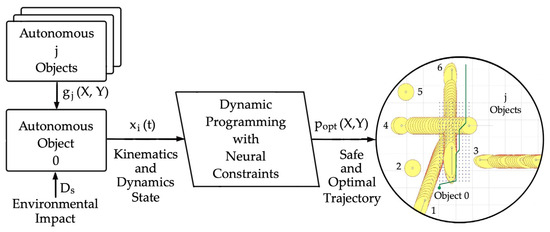
Figure 1.
Functional diagram for determining a safe and optimal trajectory of an autonomous object 0 with other autonomous j objects at safe distance Ds using the dynamic programming method with neural constraints on the process state.
2.1. Object 0 State Equations
The state equations of the object 0 motion control process are expressed in the following form:
where x is the state variable, u is the control, and t is the time, consisting of the kinematics and dynamics equations of its movement under the influence of rudder deflection α and changes in the propeller’s rotational speed n.
The kinematics of the movement of object 0 consists of the change in the time of its position coordinates p(X,Y):
As an astatic control object in the ψ0 course of anti-collision maneuvering using larger rudder deflections α, object 0 has the non-linear static characteristics , as shown in Figure 2.
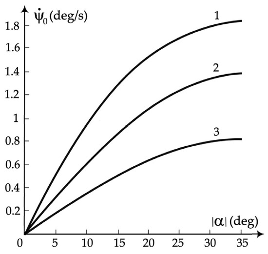
Figure 2.
Static characteristics of MASS objects: (1) 18,000 DWT container ship; (2) 32,000 DWT bulk carrier; and (3) 140,000 DWT tanker.
The static characteristic is identified during the spiral test of the object. Then, via regression analysis, the following mathematical description is obtained:
Considering the above, the following second-order non-linear model of the object’s 0 dynamics is maintained:
where T1 is the time constant of the change in object 0’s course ψ0 resulting from the rudder deflection α, and k1 is the gain coefficient.
The dynamics of object 0 during the anti-collision maneuvering of its speed V0 can be described with the following linear differential equation:
where T2 is the time constant, and k2 is the gain coefficient.
To sum up, the general state Equation (1) of the object 0 control process takes the following form:
where (x1, x2) are coordinates (X, Y) of object 0’s position; x3 is object 0’s course ψ0; x4 is the angular velocity of object 0’s turn ; x5 is object 0’s velocity; x6 is the time; u1 is the rudder angle; and u2 is the rotational speed of propeller n.
2.2. Objects j Constraints
In the process model, the passed objects j constitute its constraints:
The following is related to the need to maintain a safe approach distance Ds:
For a stationary object, the over-approach area will have the shape of a circle with a radius equal to the safe passing distance Ds under the given actual environmental conditions. For a moving object, we can choose the shape of the over-zoom area to consider the COLREG right-of-way rules. They separately apply to conditions of good visibility and limited visibility.
In good visibility conditions, object 0 must give way to object j on the right. However, if we encounter object j from the left, we expect it to give way to us. In conditions of limited visibility, the principle of giving way to the road on the right does not apply; only the increased value of the safe passing distance Ds applies. Then, the area of excessive approximation is assumed to be a circle with radius Ds.
The circular over-zoom area, as shown in Figure 3a, is described via the following relationship:
where (Xj, Yj) are the coordinates of the distance Dj of object j from object 0.
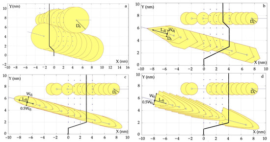
Figure 3.
Forms of constraints of the state control process as areas of excessive approximation of object j: (a) circular; (b) hexagonal and circular; (c) ellipsoidal and circular; and (d) parabolic and circular; safe trajectory.
This article aimed to show how the shape of the area of excessive approach to object j affects the course of the determined safe and optimal trajectory of object 0.
Four forms of constraints gj are proposed in conditions of good visibility: circular for objects j moving on the left; and hexagonal, elliptical, and parabolic for objects j moving on the right.
The dimensions of the hexagon, shown in Figure 3b, are determined by the dynamic length Ld and width Wd of object j:
where Lj and Wj are the length and width of object j, and Vj is the speed of object j.
The ellipse-shaped area, as shown in Figure 3c, is defined with the following inequality:
The parabolic area of the excessive approximation of object j, as shown in Figure 3d, is described with the following relationship:
where S is the span of the parabola arms.
3. Optimization of Safe Trajectory
The multi-object optimal control task formulated above consists of the state Equations (7)–(12) of object 0 containing the equations of its kinematics and dynamics, as well as the time-varying constraints (8) of the safe control process assigned to individual j objects. Many dynamic optimization methods can be used to solve this control problem, including Pontryagin’s maximum principle and Bellman’s optimality principle. The differences between these methods were described by Bokanowski et al. in [31].
Considering the multi-object control model formulated above, the most appropriate optimization method to use is the dynamic programming method based on the Bellman optimality principle.
3.1. Bellman’s Optimality Principle
The dynamics of the object are described with state Equation (1), which takes the following discrete form:
which describes the evolution of the state from time i to i + 1, taking into account the control
The trajectory is a sequence of states X {x0, x1, …, xN} and their corresponding controls {u0, u1, …, uN−1} satisfying the state Equation (1). The total cost C of the control process is the sum of the current cost cr and the final cost cf incurred when moving the object from state x0 and applying control until reaching the N horizon:
The solution to the optimal control problem is to minimize the control sequence:
Let i {ui, ui+1, …, uN−1} be a control sequence. Then, the cost of implementing the control process Ci is the sum of the component costs from i to N:
The cost value at time i is the optimal implementation cost starting from x:
The end-time cost value is defined as .
At the final moment, the current cost is the implementation time of the optimal trajectory cr = topt, and the final cost is the final deviation of the trajectory from the initial direction of movement of the object cf = d.
Figure 4 shows the computational grid for the dynamic programming of the safe and minimum-time trajectory of object 0 according to the smallest path losses for safely passing the encountered j objects.
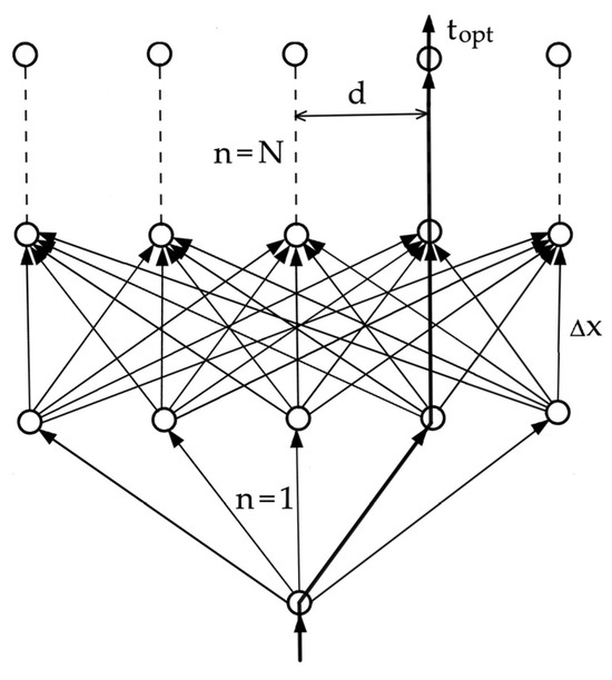
Figure 4.
Dynamic programming mesh for object 0’s optimal trajectory, where topt is optimal as the minimum time of the object’s movement; d is the deviation of the optimal trajectory from the initial direction of movement of object 0; Δx is the density of the dynamic programming mesh; and n is the number of the calculation stage.
According to Bellman’s optimality principle, which is the basis of dynamic programming, optimal control from a given moment t to the final moment depends only on the current state of the process and control and does not depend on previous states and controls:
taking into account the constraints (8) of the control process state.
3.2. Algorithm
To determine the optimal trajectory of object 0 in situations of safely passing encountered j objects, an appropriate control algorithm was synthesized in MATLAB 2023 version software, the functional diagram of which is presented in Figure 5.
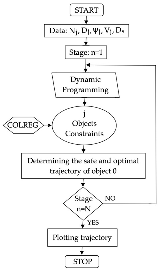
Figure 5.
Block diagram of the dynamic programming algorithm for the safe and optimal trajectory of object 0 when passing other j objects.
The state plane is divided along the path of object 0 into N stages, and each stage is divided into nodes. At each node, the movement time from the previous node is calculated.
At the same time, according to Algorithm 1, areas of excessive proximity are determined at the time of stay in a given node.
| Algorithm 1: Hexagon, ellipse, parabola, and circle domains calculation |
Begin
|
If a given node is within the bounding box of object j, a penalty of 106 s is taken as the movement time. Then, the calculation of the object’s displacement time is repeated for each subsequent node and possible path between nodes. Before moving on to the next node, the smallest shift time value and node number are selected and stored. In the last stage, as many possible paths will be determined as there are nodes at one stage, from which the path with the smallest time to move the object from the starting node to the final node is selected. By connecting subsequent nodes from end to beginning, an optimal safe trajectory of the object is obtained.
However, the areas of excessive zoom in the form of a circle, hexagon, ellipse, and parabola do not have a constant size but increase as object j approaches object 0. An artificial neural network was used for this purpose, the output of which constitutes the risk of collision with a given object, as shown in Figure 6 [32].
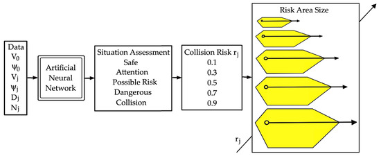
Figure 6.
An artificial neural network that adjusts the size of the possible collision area depending on the collision risk value.
The neural network, implemented in MATLAB 2023 version software in the Neural Network Toolbox, consists of three layers of neurons, with non-linear activation functions in the first and second layers and a sigmoid activation function in the third output layer. To learn it via experienced navigators, an error propagation algorithm with an adaptive learning rate and momentum was used.
In the last stage N of calculations, the path with the smallest object 0 travel time topt is selected, and the entire trajectory to the beginning is determined. In this way, a safe and optimal trajectory of object 0 is obtained when passing encountered j objects.
The dynamic programming method discussed in this article differs in the generation of time-varying constraints on the state of the control process by an artificial neural network from other similar applications, for example, those presented by Shi et al. in [33,34] regarding the Q-learning algorithm for a batch tracking fault-tolerant process.
4. Computer Simulation
Simulation studies of safe object control algorithms in collision situations were conducted using the Automatic Radar Plotting Aid (ARPA) laboratory simulator software or in Matlab/Simulink 2024a software based on real navigation situations previously recorded on the object.
The evaluation of the developed algorithm for determining a safe and optimal trajectory was carried out via a computer simulation of the example of a navigation situation of passing object 0 with j = 6 encountered objects (Table 1).

Table 1.
Values, measured in the ARPA anti-collision system, of the state variables of the process of controlling the movement of object 0 and j = 6 passing objects.
First, the courses of safe and optimal trajectories of object 0 in good visibility conditions were calculated for various forms of excessive approach areas: hexagonal and circular (Figure 7a), parabolic and circular (Figure 7b), elliptical and circular (Figure 7c), and only circular (Figure 7d).
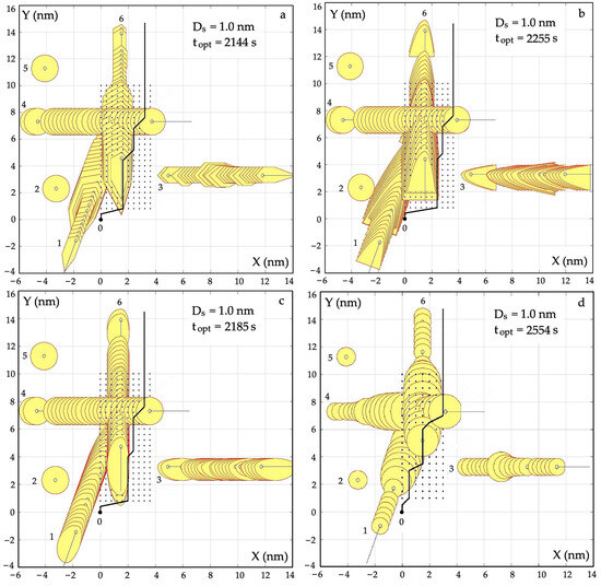
Figure 7.
Safe and optimal trajectories of object 0 for various forms of passed j object domains: (a) hexagon and circle; (b) parabola and circle; (c) ellipse and circle; and (d) circle.
Comparing the safe and optimal object trajectories for various forms of closest approach areas, it can be concluded that the lowest value of the optimization criterion is provided by circular areas, and the smallest by hexagonal areas.
Then, safe and optimal trajectories of object 0 were determined in conditions of limited visibility when maneuvering by only changing the course of object 0 (Figure 8a), and when maneuvering by changing the course and speed (Figure 8b).
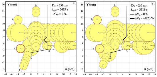
Figure 8.
Safe and optimal object 0 trajectories for circular domains of passing j objects during (a) heading maneuvering and (b) heading and speed maneuvering.
Another simulation of the algorithm was performed for a larger number of encountered objects j to show an important advantage of the dynamic programming of a safe and optimal trajectory of object 0. Namely, the more constraints assigned to each object j, the shorter the trajectory calculation time.
Figure 9a shows the safe and optimal trajectory of object 0 in conditions of good visibility, and Figure 9b in conditions of limited visibility.
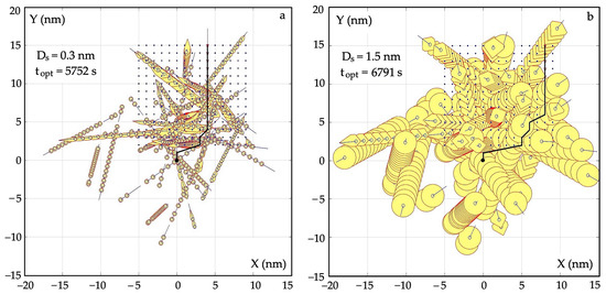
Figure 9.
Comparison of the optimal trajectories of object 0 while safely passing j = 34 objects at a safe distance (a) of Ds = 0.3 nm and (b) of Ds = 1.5 nm.
An important test for evaluating dynamic programming algorithms is the examination of their sensitivity to changes in various parameters of the control process [35,36,37].
This paper examines the sensitivity of the optimal trajectory both to the inaccuracy of the input data and changes in environmental conditions, and to the density of the dynamic programming mesh.
The measure of sensitivity s was the relative change in the optimal time topt of the safe and optimal trajectory of object 0 caused by a change in the selected parameter of the control process p:
As a result of repeated simulations of the algorithm for determining the safe trajectory of object 0, the sensitivity characteristics s of the topt criterion optimization to changes in the following parameters were obtained: the velocity δV and course δψ of object 0 (Figure 10), the velocity δVj and course δψj of object j (Figure 11), the distance δDj and bearing δNj to object j (Figure 12), the distance Ds of safe passing of objects 0 and j, and the mesh density Δx of dynamic programming (Figure 13).
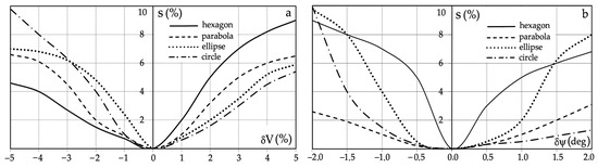
Figure 10.
Sensitivity characteristics s of the safe optimal control to data inaccuracy: (a) velocity δV of object 0; (b) course δψ of object 0.
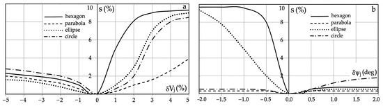
Figure 11.
Sensitivity characteristics s of the safe optimal control to data inaccuracy: (a) velocity δVj of object j; (b) course δψj of object j.
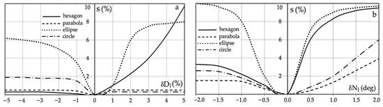
Figure 12.
Sensitivity characteristics s of the safe optimal control to data inaccuracy: (a) distance δDj to object j; (b) bearing δNj to object j.
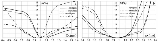
Figure 13.
Sensitivity characteristics s of the safe optimal control to (a) safe distance Ds; (b) dynamic programming mesh density Δx.
Due to the inaccuracy of the measurements of the speed V and course ψ of object 0, the greatest sensitivity s of the optimization occurs for hexagonal areas and the lowest for parabolic areas of the closest approximation of objects 0 and j.
Similarly, with the inaccuracy of the measurements of the speed Vj and course ψj of object j, the greatest sensitivity of the optimization occurs for hexagonal areas and the lowest for parabolic areas of the closest approximation of objects 0 and j.
However, with the inaccuracy of the measurements of the distance Dj and bearing Nj to object j, the greatest sensitivity of optimization occurs for ellipsoidal areas and the lowest for parabolic areas of the closest approach of objects 0 and j.
When increasing the value of the safe passing distance Ds, circular areas of the closest proximity of objects 0 and j cause the greatest optimization sensitivity, and hexagonal areas of the closest proximity to objects 0 and j cause the least.
However, when reducing the value of the safe passing distance Ds, the hexagonal areas of the greatest proximity of objects 0 and j cause the greatest optimization sensitivity, while the parabolic areas of the closest proximity of objects 0 and j cause the least.
5. Conclusions
The synthesis of the optimization of the safe and optimal trajectory of an object when passing other encountered objects according to the Bellman optimality principle, and then its presentation as an appropriate control algorithm and its simulation studies allow the following conclusions to be formulated:
- It is possible to formulate an adequate model of the actual multi-object control process, which allows for its optimization while maintaining safe traffic conditions;
- Optimization using the Bellman optimality principle in a non-linear model of the control process correctly reproduces the kinematics and dynamics of moving objects;
- The limitations of the optimality principle allow for an adequate representation of the actual control process;
- By formulating various forms of limitations in the over-approach areas, it is possible to select their best form ensuring the least sensitivity to changes in the parameters of the control process;
- The optimality principle algorithm allows us to consider a larger number of objects whose data come from ARPA anti-collision radar systems;
- The stability of safe control is ensured in the real facility by the heading change PID controller with selected optimal settings, for example, according to the Ziegler–Nichols stability criterion.
- The effect of the developed method of optimizing the object’s trajectory is the current mapping of the collision risk through the size of the neural areas of prohibited maneuvers;
- The advantage of the dynamic programming algorithm compared to the second basic optimization method is that the maximum principle is its computational efficiency in real time of the control process; thus, the more state constraints assigned to each encountered object, the shorter the time to determine its safe trajectory.
Future research on the presented topic may include the following:
- Other forms of process state constraints;
- Adapting the final conditions of the trajectory optimization task to the course of the actual control process;
- A comparison of the results of object trajectory optimization according to the optimality principle with optimization results obtained using other static, dynamic, and game optimization methods.
Funding
This research was funded by the research project “Development of control and optimization methods for use in robotics and maritime transport” No. WE/2024/PZ, Electrical Engineering Faculty, Gdynia Maritime University, Poland.
Data Availability Statement
This study did not report any data.
Conflicts of Interest
The author declares no conflicts of interest.
References
- Bellman, R.E. Dynamic Programming; Dover Publication: Mineola, NY, USA, 2003; ISBN 0-486-42809-5. [Google Scholar]
- Miretti, F.; Misul, D.; Spessa, E. DynaProg: Deterministic Dynamic Programming solver for finite horizon multi-stage decision problems. SoftwareX 2021, 14, 100690. [Google Scholar] [CrossRef]
- Sundström, O.; Guzzella, L. A generic dynamic programming Matlab function. In Proceedings of the 2009 IEEE Control Applications (CCA) & Intelligent Control (ISIC), St. Petersburg, Russia, 8–10 July 2009; pp. 1625–1630. [Google Scholar] [CrossRef]
- Mikolajczak, B.; Rumbut, J.T. Distributed dynamic programming using concurrent object-orientedness with actors visualized by high-level Petri nets. Comput. Math. Appl. 1999, 37, 23–34. [Google Scholar] [CrossRef][Green Version]
- Luus, R. Dynamic Programming: Optimal Control Applications. In Encyclopedia of Optimization; Floudas, C., Pardalos, P., Eds.; Springer: Boston, MA, USA, 2008. [Google Scholar] [CrossRef]
- Rempel, M.; Shiell, N.; Tessier, K. An approximate dynamic programming approach to tackling mass evacuation operations. In Proceedings of the 2021 IEEE Symposium Series on Computational Intelligence (SSCI), Orlando, FL, USA, 5–7 December 2021; pp. 1–8. [Google Scholar] [CrossRef]
- Gong, Z.; He, B.; Liu, G.; Zhang, X. Solution for Pursuit-Evasion Game of Agents by Adaptive Dynamic Programming. Electronics 2023, 12, 2595. [Google Scholar] [CrossRef]
- Szuster, M.; Gierlak, P. Globalized Dual Heuristic Dynamic Programming in Control of Robotic Manipulator. Appl. Mech. Mater. 2016, 817, 150–161. [Google Scholar] [CrossRef]
- Szuster, M.; Gierlak, P. Approximate Dynamic Programming in Tracking Control of a Robotic Manipulator. Int. J. Adv. Robot. Syst. 2016, 13, 16. [Google Scholar] [CrossRef]
- Kang, D.J.; Jung, M.H. Road lane segmentation using dynamic programming for active safety vehicles. Pattern Recognit. Lett. 2003, 24, 3177–3185. [Google Scholar] [CrossRef]
- Sundstrom, O.; Ambuhl, D.; Guzzella, L. On Implementation of Dynamic Programming for Optimal Control Problems with Final State Constraints. Oil Gas Sci. Technol. 2009, 65, 91–102. [Google Scholar] [CrossRef]
- Silva, J.E.; Sousa, J.B. A dynamic programming approach for the motion control of autonomous vehicles. In Proceedings of the 49th IEEE Conference on Decision and Control (CDC), Atlanta, GA, USA, 15–17 December 2010; pp. 6660–6665. [Google Scholar] [CrossRef]
- Wei, Y.; Avci, C.; Liu, J.; Belezamo, B.; Aydın, N.; Li, P.; Zhou, X. Dynamic programming-based multi-vehicle longitudinal trajectory optimization with simplified car following models. Transp. Res. Part B Methodol. 2017, 106, 102–129. [Google Scholar] [CrossRef]
- Deshpande, S.R.; Jung, D.; Canova, M. Integrated Approximate Dynamic Programming and Equivalent Consumption Minimization Strategy for Eco-Driving in a Connected and Automated Vehicle. arXiv 2020, arXiv:2010.03620v1. [Google Scholar] [CrossRef]
- Lin, S.C.; Hsu, H.; Lin, Y.Y.; Lin, C.W.; Jiang, I.H.R.; Liu, C. A Dynamic Programming Approach to Optimal Lane Merging of Connected and Autonomous Vehicles. In Proceedings of the 2020 IEEE Intelligent Vehicles Symposium (IV), Las Vegas, NV, USA, 19 October 2020–13 November 2020; pp. 349–356. [Google Scholar] [CrossRef]
- Wang, H.; Hu, C.; Zhou, J.; Feng, L.; Ye, B.; Lu, Y. Path tracking control of an autonomous vehicle with model-free adaptive dynamic programming and RBF neural network disturbance compensation. Proc. Inst. Mech. Eng. Part D J. Automob. Eng. 2022, 236, 825–841. [Google Scholar] [CrossRef]
- Lin, Z.; Ma, J.; Duan, J.; Li, S.E.; Ma, H.; Cheng, B.; Lee, T.H. Policy Iteration Based Approximate Dynamic Programming Toward Autonomous Driving in Constrained Dynamic Environment. IEEE Trans. Intell. Transp. Syst. 2023, 24, 5003–5013. [Google Scholar] [CrossRef]
- Gjorshevski, H.; Trivodaliev, K.; Kosovic, I.N.; Kalajdziski, S.; Stojkoska, B.R. Dynamic Programming Approach for Drone Routes Planning. In Proceedings of the 26th Telecommunications Forum (TELFOR), Belgrade, Serbia, 20–21 November 2018; pp. 1–4. [Google Scholar] [CrossRef]
- Bouman, P.; Agatz, N.; Schmidt, M. Dynamic programming approaches for the traveling salesman problem with dron. Networks 2018, 72, 4. [Google Scholar] [CrossRef]
- Flint, M.; Fernandez, E. Approximate Dynamic Programming Methods for Cooperative UAV Search. IFAC Proc. Vol. 2005, 38, 59–64. [Google Scholar] [CrossRef]
- Azam, M.A.; Dey, S.; Mittelmann, H.D.; Ragi, S. Decentralized UAV Swarm Control for Multitarget Tracking using Approximate Dynamic Programming. In Proceedings of the 2021 IEEE World AI IoT Congress, AIIoT 2021, Virtual Conference, 10–13 May 2021; Paul, R., Ed.; Institute of Electrical and Electronics Engineers Inc.: Piscataway, NJ, USA, 2021. Article 9454229. pp. 457–461. [Google Scholar] [CrossRef]
- Din, A.F.U.; Akhtar, S.; Maqsood, A.; Habib, M.; Mir, I. Modified model free dynamic programming: An augmented approach for unmanned aerial vehicle. Appl. Intell. 2023, 53, 3048–3068. [Google Scholar] [CrossRef]
- Jennings, A.L.; Ordonez, R.; Ceccarelli, N. Dynamic programming applied to UAV way point path planning in wind. In Proceedings of the IEEE International Conference on Computer-Aided Control Systems, San Antonio, TX, USA, 8–12 December 2008; pp. 215–220. [Google Scholar] [CrossRef]
- Vibhute, S. Adaptive Dynamic Programming Based Motion Control of Autonomous Underwater Vehicles. In Proceedings of the 5th International Conference on Control, Decision and Information Technologies (CoDIT), Thessaloniki, Greece, 10–13 April 2018; pp. 966–971. [Google Scholar] [CrossRef]
- Chen, T.; Khurram, S.; Zoungrana, J.; Pandey, L.; Chen, J.C.Y. Advanced controller design for AUV based on adaptive dynamic programming. Adv. Comput. Des. 2020, 5, 233–260. [Google Scholar] [CrossRef]
- Che, G.; Hu, X. Optimal trajectory-tracking control for underactuated AUV with unknown disturbances via single critic network based adaptive dynamic programming. J. Ambient Intell. Hum. Comput. 2023, 14, 7265–7279. [Google Scholar] [CrossRef]
- Wei, S.; Zhou, P. Development of a 3D Dynamic Programming Method for Weather Routing. TransNav Int. J. Mar. Navig. Saf. Sea Transp. 2012, 6, 79–85. [Google Scholar]
- Geng, X.; Wang, Y.; Wang, P.; Zhang, B. Motion Plan of Maritime Autonomous Surface Ships by Dynamic Programming for Collision Avoidance and Speed Optimization. Sensors 2019, 19, 434. [Google Scholar] [CrossRef] [PubMed]
- Esfahani, H.N.; Szlapczynski, R. Robust-adaptive dynamic programming-based time-delay control of autonomous ships under stochastic disturbances using an actor-critic learning algorithm. J. Mar. Sci. Technol. 2021, 26, 1262–1279. [Google Scholar] [CrossRef]
- Mi, Y.; Shao, K.; Liu, Y.; Wang, X.; Xu, F. Integration of Motion Planning and Control for High-Performance Automated Vehicles Using Tube-based Nonlinear MPC. IEEE Trans. Intell. Veh. 2023, 1, 1–16. [Google Scholar] [CrossRef]
- Bokanowski, O.; Desilles, A.; Zidani, H. Relationship between maximum principle and dynamic programming in presence of intermediate and final state constraints. ESAIM Control Optim. Calc. Var. 2021, 27, 91. [Google Scholar] [CrossRef]
- Francelin, R.; Kacprzyk, J.; Gomide, F. Neural Network Based Algorithm for Dynamic System Optimization. Asian J. Control. 2001, 3, 131–142. [Google Scholar] [CrossRef]
- Shi, H.; Gao, W.; Jiang, X.; Su, C.; Ping, L. Two-dimensional model-free Q-learning-based output feedback fault-tolerant control for batch processes. Comput. Chem. Eng. 2024, 182, 108583. [Google Scholar] [CrossRef]
- Shi, H.; Lv, M.; Jiang, X.; Su, C.; Li, P. Optimal tracking control of batch processes with time-invariant state delay: Adaptive Q-learning with two-dimensional state and control policy. Eng. Appl. Artif. Intell. 2024, 132, 108006. [Google Scholar] [CrossRef]
- Russell, S.O.D. Sensitivity analysis with dynamic programming. Can. J. Civ. Eng. 1984, 11, 1–7. [Google Scholar] [CrossRef]
- Tan, C.H.; Hartman, J.C. Sensitivity Analysis and Dynamic Programming; Wiley Online Library: Hoboken, NJ, USA, 2011. [Google Scholar] [CrossRef]
- Kumabe, S.; Yoshida, Y. Average Sensitivity of Dynamic Programming. arXiv 2021, arXiv:2111.02657. [Google Scholar]


Disclaimer/Publisher’s Note: The statements, opinions and data contained in all publications are solely those of the individual author(s) and contributor(s) and not of MDPI and/or the editor(s). MDPI and/or the editor(s) disclaim responsibility for any injury to people or property resulting from any ideas, methods, instructions or products referred to in the content. |
© 2024 by the author. Licensee MDPI, Basel, Switzerland. This article is an open access article distributed under the terms and conditions of the Creative Commons Attribution (CC BY) license (https://creativecommons.org/licenses/by/4.0/).