Article

Analysis of Phase-Locked Loop Filter Delay on Transient Stability of Grid-Following Converters

The College of Electrical Engineering, Xinjiang University, Urumqi 830046, China
*
Author to whom correspondence should be addressed.
Electronics 2024, 13(5), 986; https://doi.org/10.3390/electronics13050986
Submission received: 10 February 2024 / Revised: 28 February 2024 / Accepted: 2 March 2024 / Published: 5 March 2024
(This article belongs to the Topic Power System Dynamics and Stability)

Abstract

:
To ensure precise phase estimation within the q-axis of the phase-locked loop (PLL), integrating a filter into the q-axis loop is essential to mitigate grid-voltage harmonics. Nevertheless, the intrinsic delay characteristics of this filter impede PLL synchronization during significant grid disturbances. This study begins by developing mathematical models for three types of filters—moving-average filter (MAF) for eliminating odd harmonic components, dq-frame cascaded delayed signal cancellation (dqCDSC) filter, and notch filter (NF). Following the reduction in filter orders, a third-order nonlinear large-signal model of the PLL, incorporating an additional q-axis internal filter, is formulated. Using phase plane analysis, this study investigates the transient synchronism of the grid-following converter (GFL) and explores the influence of delay time constants from the three PLL filters on its behavior while delineating the boundaries of their basins of attraction. Theoretical findings indicate that, relative to the traditional SRF-PLL, incorporating an internal filter into the PLL compromises the transient synchronous stability of GFL. Specifically, greater filter delay time constants exacerbate the GFL’s vulnerability to transient instability amid substantial grid disturbances. Hence, careful consideration is essential when using MAF-PLL and NF-PLL in situations demanding high synchronization stability. The theoretical analyses are validated using Matlab/Simulink to verify their accuracy.

1. Introduction

To fulfill the strategic goal of establishing a new power system primarily reliant on renewable energy sources [1,2], grid-connected converters have emerged as a pivotal interface, enabling the swift advancement of renewable energy generation [3]. Consequently, it has progressively supplanted synchronous generator power as the primary energy source within the power grid. This transformative shift has ushered in a “double high” trend within the power system, characterized by a significant presence of both renewable energy sources and power electronic equipment [4]. The reliable and secure operation of such “double high” systems critically hinges on the effective performance of grid-connected converters. In recent years, stability concerns surrounding grid-connected converters have garnered significant attention, notably in the aftermath of incidents such as the UK’s 8.9 blackout and the 2021 Texas blackout [5,6].
At present, the predominant synchronization control strategies for grid-connected converters involve proportional-resonant (PR) control in the αβ coordinate system [7,8,9] and proportional-integral (PI) control with phase-locked loops (PLLs) synchronization in the dq coordinate system, attributed to the enhanced robustness of PI control. As a result, the PLL synchronization control strategy is uniformly applied across wind and photovoltaic grid-connected converters. Grid-connected converters employing PLL synchronization are also known as grid-following converters (GFLs). The current implementation of GFL heavily relies on PLL to monitor the grid-voltage phase at the point of connection (POC) for grid synchronization [10]. The voltage present at the POC is equivalent to the voltage output by the GFL. Consequently, the dynamic characteristics of the PLL significantly influence the grid-tied stability of the GFL [11]. References [12,13] advocate for integrating a filter into the PLL’s q-axis control loop to enhance the GFL’s stability, under minor disturbances in high harmonic grid environments. Moreover, the literature [14] suggests the incorporation of a notch filter (NF) or multiple NFs into the PLL control loop to eliminate harmonic components selectively. Reference [15] explores the use of a moving-average filter (MAF) within the PLL control loop, functioning as both a linear phase filter and, under certain conditions, an ideal low-pass filter. Additionally, in reference [16], the investigation into repetitive regulators (RRs) within the PLL control loop demonstrates their efficacy in attenuating harmonic components and providing rapid dynamic responses to disturbances. Proposing delayed signal cancellation, reference [17,18] introduces the dq-frame cascaded delayed signal cancellation (dqCDSC) to enhance PLL’s phase-locking performance under high harmonic grid conditions. Additionally, in addressing approaches to attenuate grid harmonics, references [19,20] focus on leveraging the inherent control strategies of GFL. They introduce a cooperative control framework based on a hybrid algorithm, aimed at mitigating the adverse effects of grid harmonics on GFL performance. However, the studies mentioned above overlook the impact of inherent filter delay characteristics on GFL’s synchronization during significant disturbances.
The synchronization stability of a converter is defined by its ability to sustain synchronization with the grid despite significant disturbances [21]. The extensive transmission distances associated with renewable energy sources and the substantial grid impedance at the POC contribute to positive feedback in the synchronization loop, amplifying synchronization instability. Reference [22] introduced the quasi-static large signal (QSLS) model to elucidate this phenomenon, leveraging phase plane analysis, the equal-area criterion, and the energy function method to dissect the synchronization stability mechanism of the GFL. In a related study, reference [23] applied the equal-area criterion, based on principles of kinetic and potential energy conservation, to assess whether the operational state during a fault could revert to stability, thereby evaluating the transient synchronization stability of the GFL. Additionally, reference [24] visually depicted transient instability phenomena without analytical tools, utilizing numerical solutions of first and second-order nonlinear system equations to graph phase trajectories. Moreover, reference [25] formulated an analytical Lyapunov energy function, deriving a more conservative stability region. Furthermore, reference [26] investigated the interaction between the current control and the PLL loop, devising a more intricate QSLS model to scrutinize transient synchronization stability. Additionally, taking into account the synergistic impact of active filters at the GFL output, current regulation, and the PLL feedback mechanism, the literature [27,28,29] introduces an advanced PLL parameterization strategy aimed at improving the synchronizing stability of GFL amidst weak grid scenarios. The modeling and analysis of transient stability in GFL typically assume an environment devoid of grid harmonics. However, real-world scenarios necessitate the integration of filters within the PLL control loop to eliminate these harmonics. During grid faults, the delay characteristics inherent in these filters can significantly influence the synchronization of GFL with the grid.

1.1. Novelty and Contribution

In this research, the impact of grid harmonics on the transient stability of GFL is included in the modeling and analysis. Diverging from the traditional presumption of a harmonics-free grid environment, this manuscript highlights the critical necessity of implementing filters within the PLL control scheme to eliminate harmonics, as well as to address the consequential effects of filter delays on the synchronizing stability of GFL systems. By exploiting the higher-order nonlinear characteristics inherent in filters, a third-order nonlinear large-signal model that integrates the filter’s PLL is developed herein. This model facilitates an investigation into the influence of varying filter delay time constants on the synchronizing stability of GFL, guiding the strategic selection of PLL filters for scenarios where enhanced synchronizing stability is imperative.

1.2. Chapter Organization

The ensuing segments of this manuscript scrutinize the ramifications of filter delays on the transient stability of GFL, structured as follows. Section 2 presents the mathematical modeling of GFL, develops mathematical models for three distinct inner-loop filters, and realizes filter model order reduction, laying the foundation for the large-signal analysis in Section 3. Section 3 investigates the mechanism underlying the effect of filter delays on the transient stability of GFL. The simulation results presented in Section 4 are used to validate the theoretical analysis provided in Section 2 and Section 3. Section 5 succinctly concludes the discourse.

2. Modeling of Synchronization Stability
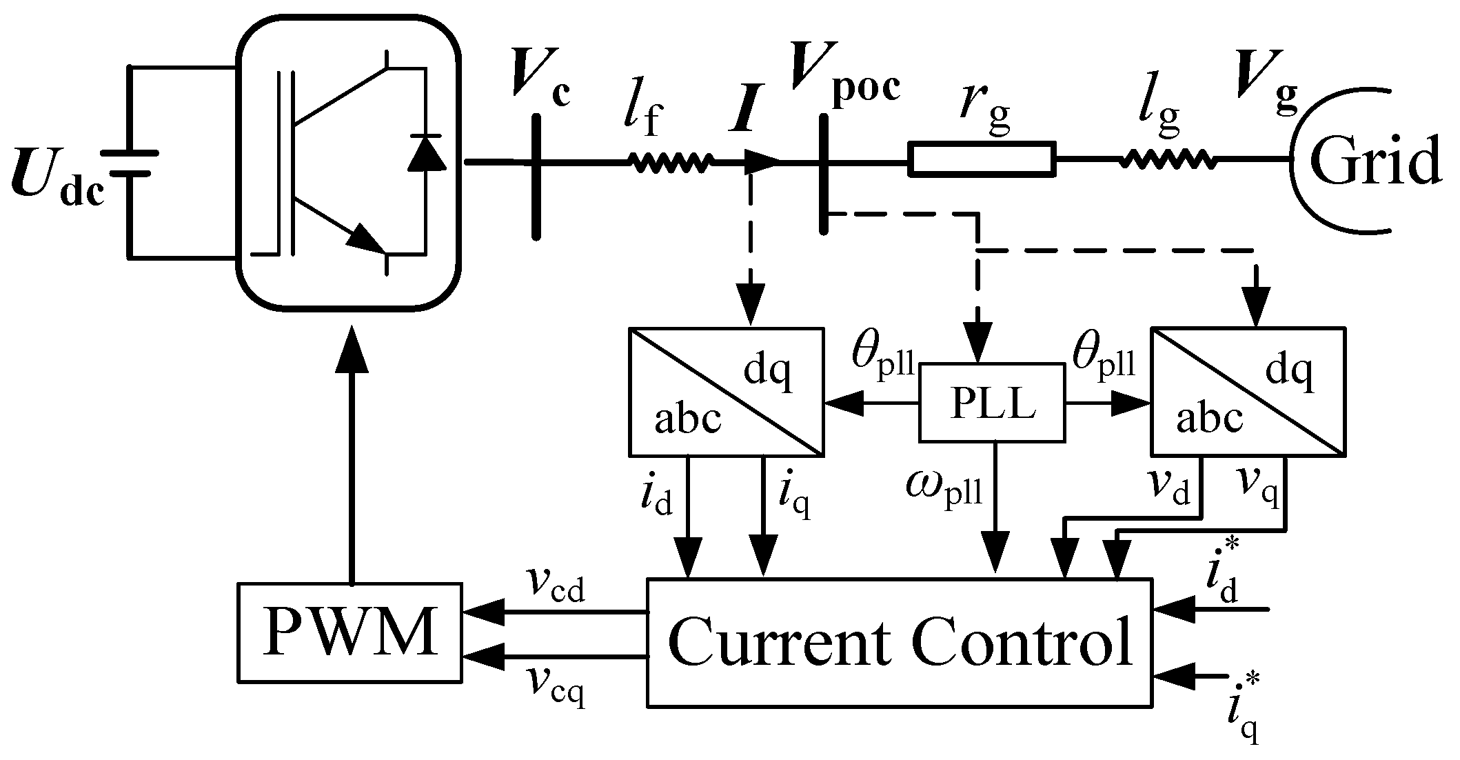
2.1. GFL Modeling

The system structure of the GFL is illustrated in Figure 1. Here, VPOC and Vg denote the voltages at the POC and the grid, respectively. The injected current into the grid is represented by I, while lf refers to the filter located at the converter’s output port. Additionally, rg and lg denote the resistance and inductance on the grid side. The DC voltage source is represented as Udc, typically maintained at a constant value. The synchronization between the GFL and the grid is achieved using the synchronous reference frame phase-locked loop (SRF-PLL), with θpll and ωpll representing its output phase angle and frequency, respectively. Current control is effected through a PI regulator, wherein kpc and kic delineate the proportional and integral coefficients of the controller, correspondingly.
The voltage at the POC can be obtained from Figure 1:
V POC = V g + I ( Z g )
where Zg represents the grid impedance, given by Z g = r g + j ω pll l g . The q-axis voltage component can be obtained by performing a Park transformation on VPOC:
V pocq = r g i q + ω pll l g i d V g sin δ
In (2), δ = θpllθg, where θg denotes the grid phase, the output current of the GFL maintains a constant reference current value i d owing to the significantly shorter time scale of the current loop control compared to the PLL. The PLL, through the application of a PI regulator, achieves grid synchronization by ensuring Vpocq = 0, as specified in its governing dynamic equation.
{ d θ pll d t = ω pll = ω g + Δ ω pll d ω pll d t = k p , pll V pocq + k i , pll V pocq d t
where ωg signifies the nominal angular frequency of the grid. If Vpocq consists solely of fundamental frequency components, the PLL can accurately estimate the grid phase by setting Vpocq = 0. Yet, if there are harmonic components in Vpocq, incorporating filters into the PLL control loop becomes essential to eliminate these components and ensure precise grid phase estimation.

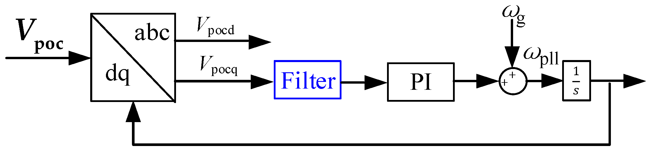
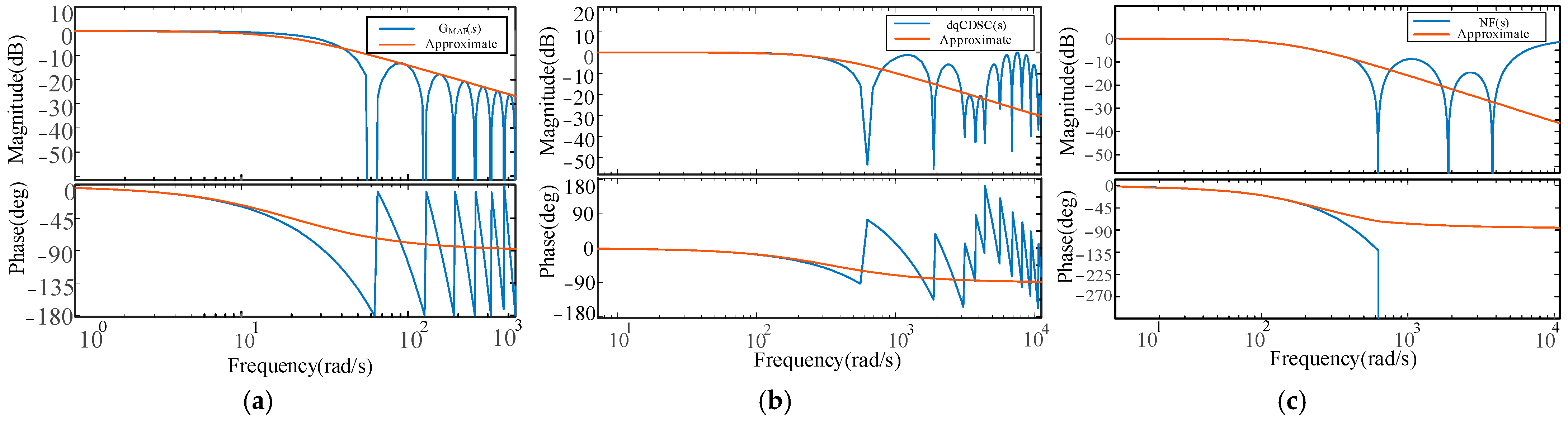
2.2. Filter Modeling

In practical scenarios, the main grid-voltage harmonic components typically include the −5th, +7th, −11th, and +13th harmonics. Even-order harmonics and the DC component are ignored due to their notably lower amplitudes, in comparison to the odd-order harmonics. Consequently, the mathematical model of the internal loop filter is primarily tailored to eliminate these specified harmonic components. Figure 2 illustrates the PLL configuration incorporating the additional internal loop filter. Given our focus on fundamental frequency synchronization, the filter exhibits delay characteristics when projected onto the low-frequency range. Therefore, subsequent discussions treat the three filters as first-order inertial elements in modeling synchronization stability.

2.2.1. MAF

The MAF, alternatively referred to as a rectangular window filter, is characterized by its transfer function in the Laplace domain, given as:
G MAF ( s ) = 1 e T w s T w s
The equation defines Tw as the window length of the MAF. MAF can eliminate DC components and frequency components that are integer multiples of 1/Tw (in Hz). When the grid voltage consists solely of odd-order harmonic components, the standard configuration for MAF’s window length is Tw = T/2, where T represents the fundamental period of the grid voltage.
When GMAF(s) is integrated into the q-axis loop of the PLL, its e T w s term becomes a non-rational function, which is not conducive to subsequent analysis of transient stability. Utilizing the first-order Pade approximation, we derive the following:
e T w s 1 T w s / 2 1 + T w s / 2        G MAF ( s ) 1 T w s / 2 + 1
The approximated transfer function yields a first-order inertial component. By defining Tw/2 = TMAF as the time delay constant of the MAF, Figure 3a is utilized to assess the accuracy of this approximation through a comparison of the Bode plot between GMAF(s) and its approximated transfer function. It is evident that the approximation effectively represents the dynamic behavior of GMAF(s).

2.2.2. dqCDSC

In the dq coordinate system, harmonic components demonstrate “half-wave symmetry”, allowing for the summation of delayed harmonic components to eliminate those injected into the q-axis loop. This process maintains the DC component in the dq coordinate system unchanged. It is referred to as dqDSC [18]. Its transfer function is as follows:
dqDSC n ( s ) = 1 2 ( 1 + e T n s )
In (6), n represents the delay factor, where its selection can prevent certain characteristic harmonic components. In most scenarios, a single dqDSC operator might be insufficient to counteract associated harmonic components. Depending on the harmonic type in the grid and existing applications, multiple dqDSC operators with specific delay factors are usually cascaded. Equation (7) describes dqCDSC in the Laplace domain, where m represents the quantity of cascaded dqDSC operators. Figure 4 illustrates the time-domain implementation of dqCDSCn1,n2,…, nm.
CDSC n 1 , n 2 , , n m ( s ) = d q DSC n 1 ( s ) × d q DSC n 2 ( s ) × × d q DSC n m ( s )  
The presence of odd-order harmonic components alone in the grid necessitates the cascading of two dqDSC operators with delay factors of n1 = 4 and n2 = 24. Consequently, the transfer function is formulated as:
dqCDSC n 1 , n 2 ( s ) = 1 2 ( 1 + e ( T / n 1 ) s ) × 1 2 ( 1 + e ( T / n 2 ) s )
Similarly, based on the first-order Pade approximation, substitute e ( T / n ) s 1 ( T 2 n ) s 1 + ( T 2 n ) s yields the following:
dqCDSC n 1 , n 2 ( s ) 1 T 2 4 n 1 n 2 s 2 + ( T 2 n 1 + T 2 n 2 ) s + 1
In the low-frequency range, the s2 term can be neglected, further yielding the following:
dqCDSC n 1 , n 2 ( s ) 1 T 2 ( 1 / n 1 + 1 / n 2 ) s + 1
The time delay constant of the dqCDSC filter is defined as TdqCDSC = T × (1/n1 + 1/n2)/2. Based on Figure 3b, the approximated outcome still predicts the dynamic behavior of its original transfer function.

2.2.3. NF

The NF is a band-stop filter designed to substantially reduce harmonic components within a defined frequency band while maintaining minimal impact on other frequency components. The transfer function representing NF [30] is:
NF ( s ) = s 2 + ω nf 2 s 2 + ( ω nf / Q ) s + ω nf 2
where ω nf represents the notch frequency and Q denotes the quality factor. To eliminate odd-order harmonic components in the phase-locked loop’s q-axis loop, cascading three NFs is necessary. Each NF has notch frequencies set, respectively, at 2π(2 × 50), 2π(6 × 50), and 2π(12 × 50)rad/s. The selection of the quality factor Q depends on the expected range of variation in the grid frequency. Reference [24] proposes that when Q is chosen as Q = 2 , NF effectively suppresses odd-order harmonic components even under significant variations in the grid frequency.
When three NFs are cascaded, the equation representing their transfer function is as follows:
NFs ( s ) = NF ω nf 1 ( s ) × NF ω nf 2 ( s ) × NF ω nf 3 ( s )
Equation (12) presents an 8th-order transfer function, which challenges mathematical simplification. Therefore, this study employs system identification techniques to fit the frequency, magnitude, and phase data obtained from the frequency domain response model in (12). Consequently, a first-order transfer function is derived through this identification process.
NFs ( s ) 125 125 + s
A comparison between the transfer functions of (12) and (13) is conducted using a Bode plot. Figure 3c illustrates that, especially in the low-frequency range, the output magnitude of the identified transfer function closely aligns with that of the original transfer function. The accuracy of the fitted results in this low-frequency spectrum indicates a close correspondence between the identified and original transfer functions.
Based on the aforementioned, the transfer functions of these three filters can be consistently represented as first-order inertial elements. Their individual time constants correspond to the delay time constants of the filters, as illustrated in Table 1.

3. Synchronization Stability Analysis

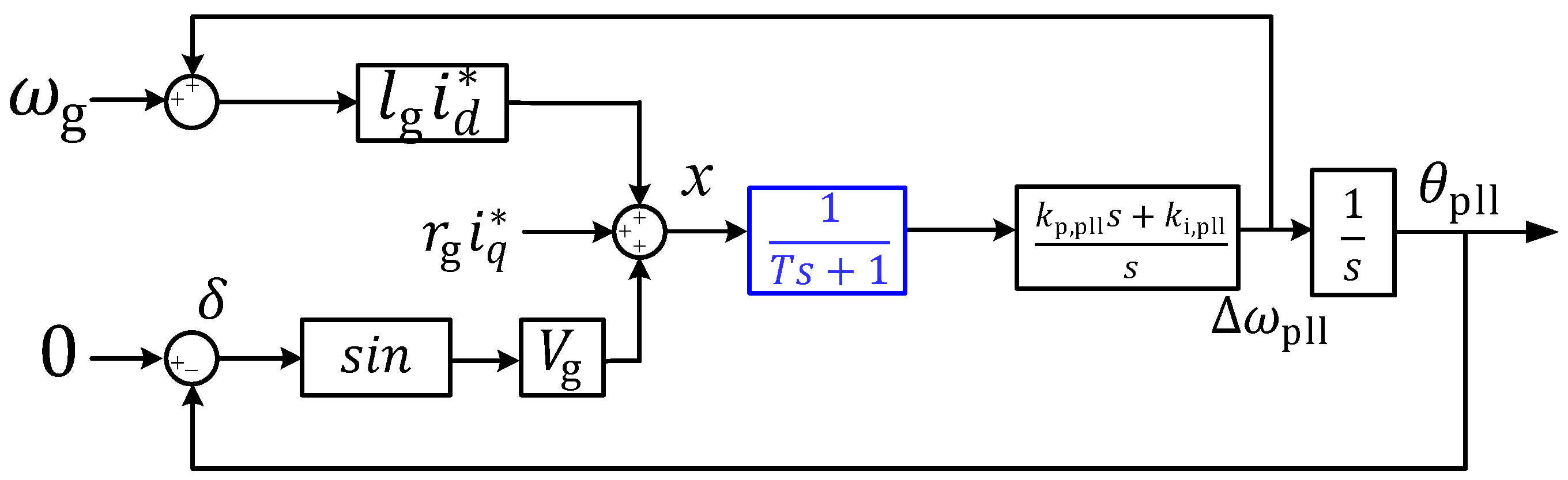
3.1. 3rd PLL QSLS Model

Derived from the reduced-order filter transfer functions in the preceding section, they can all be equivalently represented as first-order inertial elements. This section initially establishes the large-signal model of the PLL incorporating a first-order inertial element [31]. The introduction of this inertial element transforms the PLL from a second-order system to a third-order system, as illustrated in Figure 5.
The output from the inertial element depicted in Figure 5 is considered the state variable x, and δ, and Δ ω p l l represent the outputs of the remaining two integrators. These three state variables collectively portray the system’s time-domain behavior. The state variables ( δ , Δ ω pll , x ) = ( x 1 , x 2 , x 3 ) are defined, facilitating the formulation of the state-space equations for the third-order PLL as depicted in (14).
{ x ˙ 1 = x 2 = f 1 x ˙ 2 = k p , pll ( r g i q + ( x 2 + ω g ) l g i d V g sin x 1 x 3 ) / T           + k i , pll x 3 = f 2 x ˙ 3 = ( r g i q + ( x 2 + ω g ) l g i d V g sin x 1 x 3 ) / T = f 3
Due to the nonlinear characteristics of the third-order PLL system integrating inertial elements, this study utilizes phase-plane analysis for numerical solutions [32]. This method, employing the ode45 algorithm, illustrates the trajectory of the numerical solution of the nonlinear system under specific initial conditions. Thus, it visually captures the system’s dynamics, stability, equilibrium points, and the influence of initial states of the system behavior.
Before analyzing transient stability, it is crucial to evaluate the existence and stability of equilibrium points during transients. Setting the state equations (14) to zero—f1 = 0, f2 = 0, f3 = 0—facilitates the determination of the system’s two equilibrium points: δ 0 ( x 10 , x 20 , x 30 ) and δ u ( π x 10 , x 20 , x 30 )
x 10 = arcsin ( r g i q + ω g l g i d V g ) , x 20 = 0 , x 30 = 0
Under the condition of V g > r g i q + ω g l g i d , δ u is always unstable. Therefore, we primarily study the stability of the equilibrium points of δ 0 and regard them as the equilibrium points for normal operation.

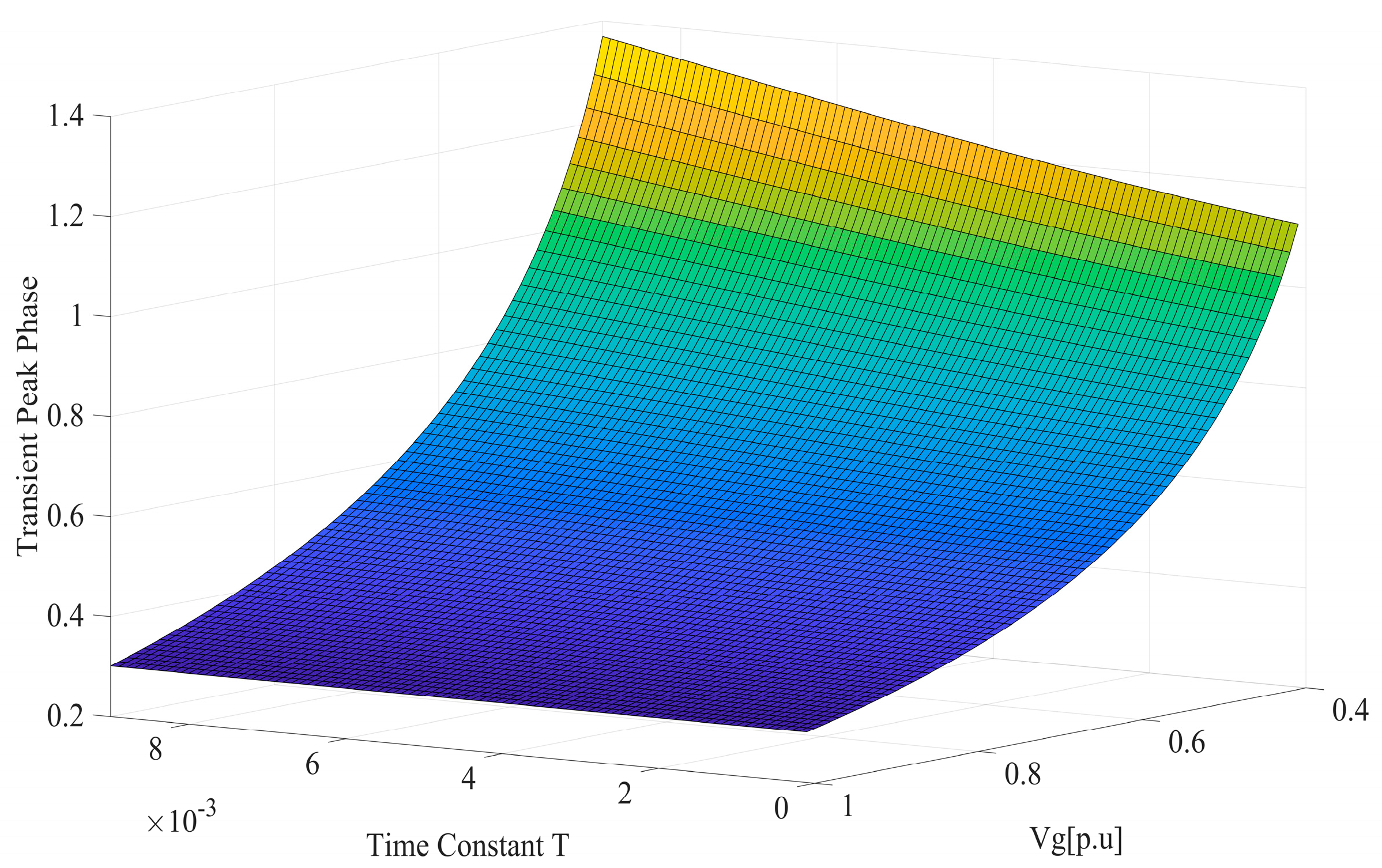
3.2. Transient Stability Analysis Due to Time Constant of the Inertial Element

In the absence of an inertial element in the q-axis loop of the PLL, when the grid-voltage amplitude drops to V g , f , the proportional component of the PI controller responds instantaneously, leading to a non-zero initial velocity Δ ω pll ( t 0 + ) and an input error V pocq ( t 0 + ) at time t 0 + .
Δ ω pll ( t 0 + ) = k p , pll ( V g , 0 V g , f ) sin δ 0 1 k p , pll l g i d
V pocq ( t 0 + ) = l g i d Δ ω pll ( t 0 + ) + ( V g , 0 V g , f ) sin δ 0
In (16) and (17), V g , 0 denotes the initial grid-voltage value, while Δ ω pll ( t 0 + ) and V pocq ( t 0 + ) are both positive values. During a sustained fault, the dynamic response of GFL is as follows:
V pocq ( t ) = l g i d Δ ω pll ( t ) + V g , 0 sin δ 0 V g , f sin ( δ 0 + 0 t 1 Δ ω pll ( t ) d t )
Δ ω pll ( t ) = k p , pll V pocq ( t ) + k i , pll 0 t 1 V pocq ( t ) d t
where t1 represents the time required for the PI controller to attain a steady state without the presence of an inertial element. When incorporating an inertial element into the q-axis loop of the PLL, the integrator within the inertial element mitigates sudden fluctuations in the state variable x3, leading to the following expression:
Δ ω ˜ pll ( t 0 + ) = 0
V ˜ pocq ( t 0 + ) = ( V g , 0 V g , f ) sin δ 0
Hence, it follows that Δ ω pll ( t 0 + ) > Δ ω ˜ pll ( t 0 + ) , V pocq ( t 0 + ) > V ˜ pocq ( t 0 + ) . The behavior of the inertial element and the PI controller throughout the fault duration is as follows:
V ˜ pocq ( t ) = 0 t 2 1 T ( V pocq ( t ) V ˜ pocq ( t ) ) d t + V pocq ( t 0 + )
Δ ω ˜ pll ( t ) = k p , pll V ˜ pocq ( t ) + k i , pll 0 t 3 V ˜ pocq ( t ) d t
where t2 and t3 denote the time needed for the inertial element and the PI controller output response to attain steady-state, respectively. Owing to the delayed response of the inertial element, t1 the time required for the PI controller to rectify the same error is shorter than t3. Furthermore, as the time constant T of the inertial element increases, the output voltage V ˜ pocq decreases, leading to an increase in integration accumulation and an elongation of the time t2 required to reach a steady state. Consequently, this results in a larger transient peak phase of the PLL. Therefore, the inclusion of the inertial element exacerbates synchronization stability.
The analysis conducted previously suggested that incorporating an inertial element led to an increase in the transient peak phase of the PLL, consequently undermining the transient synchronization stability of the GFL. To formulate comprehensive conclusions, this study incorporates the parameters outlined in Section 4 into the transient stability analysis model. Subsequently, numerical techniques are employed to calculate the transient peak phase of the PLL, varying Vg and T, as depicted in Figure 6. The surface plot demonstrates that, as the magnitude of the voltage drop rises, the transient peak phase similarly increases, particularly with larger time constants associated with the inertial element.

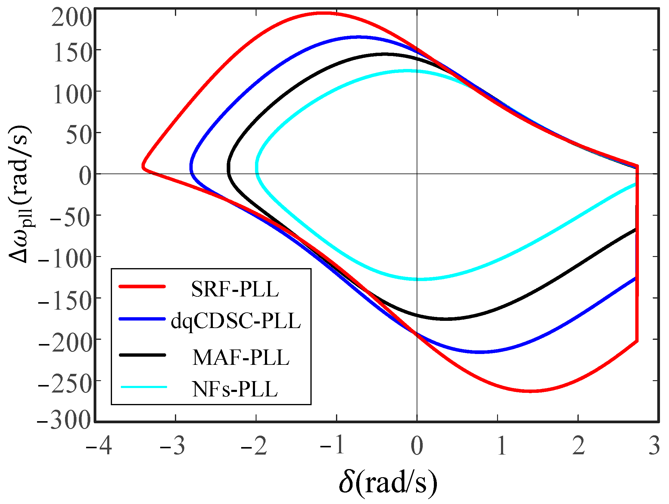
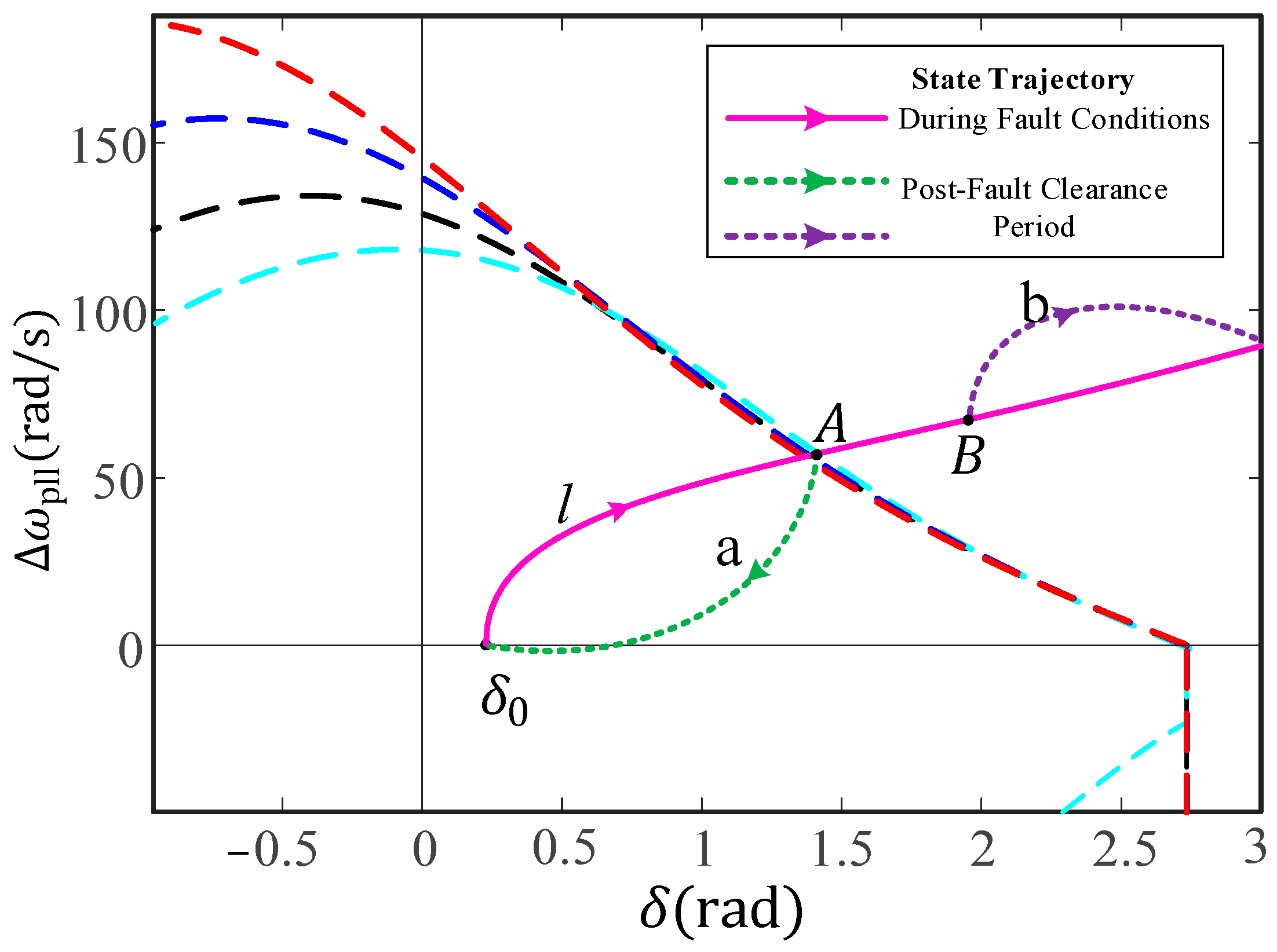
3.3. Estimation of Attraction Domains

In the domain of large-signal systems, the detection of equilibrium points amidst transient conditions does not guarantee stability during such periods. It is critical to delineate the extent of ‘attraction’ for these points, defined as the domain of attraction. If the initial state and trajectory of the system deviate from this domain, the risk of transient instability becomes imminent. Therefore, the domain of attraction underscores the system’s capability to counteract disturbances, serving as an indispensable index for evaluating system stability [25,33]. Depicted in Figure 7 are the basins of attraction for the SRF-PLL and three additional filters within the PLL, calculated using the ode45 algorithm and parameters specified in Section 4. The order of the basin areas, ranked from largest to smallest, is SSRF-PLL > SdqCDSC-PLL > SMAF-PLL > SNFs-PLL. This observation implies that as the filter delay time constants increase, the basin area decreases. Larger filter delay time constants exacerbate transient synchronization stability issues.
To validate the accuracy of the attraction domain delineated, we consider the NFs-PLL as an exemplar. When the grid voltage plummets to 0.05 p.u, the absence of equilibrium points in the system signifies instability. The trajectory during the fault event is depicted [34,35] as curve l in Figure 8. Subsequently, upon reaching point A after 37.62 ms, coinciding with the fault clearance, the system follows trajectory a, ultimately reverting to the equilibrium point. However, upon reaching point B after 45.2 ms, although the fault is rectified, the post-fault trajectory deviates along path b, resulting in transient instability. The attraction domain illustrated in this study exhibits a degree of conservatism. However, this conservative approach provides a safety buffer in fault detection and clearance, mitigating the risk of undetected GFL instability resulting from grid faults. This, in turn, helps prevent situations where protective devices fail to trigger, thereby averting the escalation of faults.
Figure 9 juxtaposes the phase trajectory plots of the SRF-PLL with three additional filter-based PLLs. When subjected to identical fault voltages, the SRF-PLL and dqCDSC-PLL, featuring smaller filter time delay constants, converge towards the post-fault equilibrium point. Conversely, the MAF-PLL and NFs-PLL, equipped with larger filter time delay constants, exhibit transient instability under the same fault scenario. The maximum phase value of the trajectory and the maximum deviation from the equilibrium point denote the transient peak phase. It is evident that during grid faults, the incorporation of additional filters leads to an escalation in the transient peak phase of the PLL. A heightened transient peak phase signifies an increased likelihood of the GFL transitioning to an unstable equilibrium point δu. Consequently, the integration of filters exacerbates the transient synchronization stability of the GFL [36,37].

4. Simulation Validation

Electromagnetic transient models (EMTs)of the GFL are individually developed in Matlab/Simulink to enhance the verification of the theoretical analysis. The parameters required for the simulation model are as detailed in Table 2.

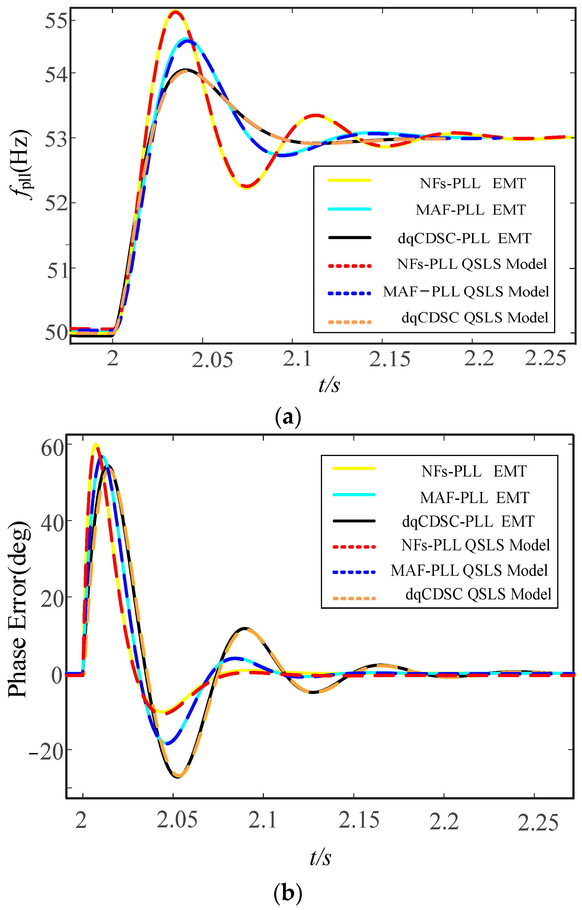
4.1. Validity Assessment of the 3rd-PLL QSLS Model

To enhance the validation of the reduced-order [38] models of the PLL incorporating three additional filters, a series of simulation experiments mimicking extreme grid faults is designed as follows: Scenario (1) entails a +3 Hz step change in the grid frequency at 2 s, whereas Scenario (2) involves an abrupt phase jump of +40° in the grid at 2 s. Subsequently, the reduced-order models are juxtaposed with the simulation outcomes of the third-order PLL QSLS model. The transient responses of the PLL frequency and the grid-phase error with the three additional filters are depicted in Figure 10 for further analysis.
As depicted in Figure 10, following a grid-frequency step change of +3Hz and a phase jump of +40°, the transient response curves closely align with those of the approximated inertial element. This alignment underscores the capability of the approximate results presented in this paper to precisely forecast the dynamic behavior of the full-order filtered PLL.

4.2. Impact of Inertial Element on Transient Synchronization Stability of GFL

In this section, we conduct a detailed analysis to ascertain and validate the influence of the inertial element on the transient stability of the GFL. Leveraging the system parameters delineated in Section 4 and the formulated QSLS model of the 3rd PLL, we proceed to explore this impact. Specifically, we initiate the examination by orchestrating a scenario where the grid voltage plummets to 0.4 p.u. at t = 2 s. Subsequently, we juxtapose the phase deviation δ and the frequency deviation Δ ω pll responses of the SRF-PLL with those of the PLL augmented by the additional inertial element, as illustrated in the accompanying figure.
From Figure 11, it is apparent that the introduction of an inertial element into the PLL control loop enhances the transient phase peak of the system. Moreover, as the time constant T of the inertial element increases, the transient peak grows larger. Conversely, analyzing the response curve of the frequency deviation Δ ω pll versus time t it is evident that upon an instantaneous fault occurrence, the incorporation of an inertial element in the PLL control loop prevents Δ ω pll from undergoing abrupt changes. Consequently, it mitigates the same error magnitude. The PLL lacking the inertial element swiftly converges to a stable value, and as T escalates, the time taken by the PLL to attain a steady state response also extends. Hence, a greater time constant T of the inertial element exacerbates the synchronization stability of the GFL.

4.3. Validation of the Effectiveness of the Attraction Domain

Figure 12 illustrates the simulation validation results derived from the theoretical analysis presented in Section 3.3. At 2 s, a simulated grid fault causes the voltage to decrease to 0.05 p.u. By 37.62 milliseconds, the fault is rectified, resulting in the resynchronization of the NFs-PLL with the grid. The NFs-PLL navigates within the basin of attraction, reconverging to the equilibrium point. However, by 45.2 milliseconds, following the clearance of the grid fault, the NFs-PLL exhibits instability, with its trajectory failing to stabilize outside the basin of attraction.

4.4. Verification of the Impact of Filter Time Constants on Transient Synchronization Stability

Figure 13 presents a comparative analysis of the phase responses between the SRF-PLL and PLLs augmented with three additional filters, with the grid voltage dropping to 0.35 p.u. While the SRF-PLL and the dqCDSC-PLL featuring smaller filter time constants maintain synchronization with the grid during this fault scenario, the incorporation of dqCDSC filters exacerbates the synchronization stability issues of the GFL. Conversely, the MAF-PLL and NF-PLL, characterized by larger filter time constants, exhibit transient instability under similar fault conditions. Consequently, caution is advised when deploying MAF-PLL and NF-PLL configurations during severe grid faults.

5. Conclusions

Reference [28] explores the challenge of voltage oscillations at the POC across differing grid strengths, proposing modifications to filter gains to mitigate voltage oscillations at grid interconnection points for GFL. While this method effectively boosts GFL’s small-signal synchronizing stability, its influence on GFL’s transient dynamics remains uncharted territory. This work aims to bridge this knowledge gap, focusing on the repercussions of integrating a filter into the q-axis control loop of the PLL on the transient synchronizing stability of GFL systems; this study formulates third-order state-space equations tailored for analyzing this issue post-reduction in the filter mathematical model. Leveraging this model, we employ phase-plane analysis to explore transient stability concerns associated with three supplemental filter PLLs: MAF-PLL, dqCDSC-PLL, and NFs-PLL. This investigation unveils the impact mechanisms of varied PLL filter time constants on the transient synchronization stability of the GFL. Subsequently, simulation experiments are executed to corroborate the insights, culminating in the following conclusions:
(1)
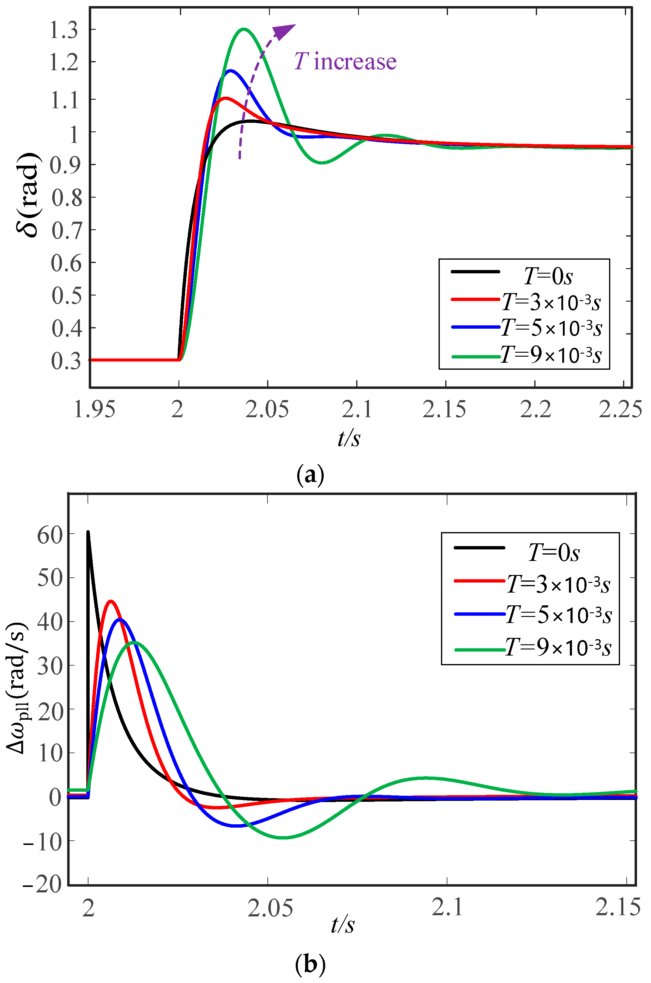
In juxtaposition with the traditional SRF-PLL, integrating a filter within the q-axis control loop of the PLL has been observed to compromise the transient stability of GFL. This phenomenon is characterized by amplified peak phase deviations during transient episodes and protracted durations for the GFL to re-establish a stable equilibrium state in the aftermath of substantial grid perturbations. Notably, the severity of these impacts escalates concomitantly with the increment in the filter’s delay time constant.
(2)
In power grids containing a significant amount of odd-order harmonics, to improve the accuracy of phase locking in the PLL while avoiding transient instability of the GFL, it is recommended to use the dqCDSC-PLL with smaller delay time constants in practice.
The conclusions drawn are rigorously validated via MATLAB/Simulink simulations, with the outcomes affirming the accuracy of the mathematical models and theoretical analyses outlined earlier.

Author Contributions

Conceptualization, C.Z. and J.C.; methodology, C.Z., J.C. and W.S.; validation, C.Z. and J.C.; data curation, C.Z. and W.S.; writing—original draft preparation, C.Z.; writing—review and editing, C.Z., J.C. and W.S.; supervision, J.C. and W.S. All authors have read and agreed to the published version of the manuscript.

Funding

The Major Science and Technology Project of the Xinjiang Uygur Autonomous Region provided funding for this study under project number 2022A01004-1. This project was also funded by the Department of Science and Technology of the Xinjiang Uygur Autonomous Region, China.

Data Availability Statement

Data are contained within the article.

Acknowledgments

The authors express their gratitude for the support provided by the Xinjiang Uyghur Autonomous Region’s major science and technology special program.

Conflicts of Interest

The authors declare no conflict of interest.

References

  1. Kroposki, B.; Johnson, B.; Zhang, Y.; Gevorgian, V.; Denholm, P.; Hodge, B.-M.; Hannegan, B. Achieving a 100% renewable grid: Operating electric Power systems with extremely high levels of variable renewable energy. IEEE Power Energy Mag. 2017, 15, 61–73. [Google Scholar] [CrossRef]
  2. Paul, S.; Dey, T.; Saha, P.; Dey, S.; Sen, R. Review on the development scenario of renewable energy in different country. In Proceedings of the 2021 Innovations in Energy Management and Renewable Resources (52042), Kolkata, India, 5–7 February 2021; pp. 1–2. [Google Scholar]
  3. Zhao, J.T.; Huang, M.; Yan, H.; Tse, C.K.; Zha, X.M. Nonlinear and Transient Stability Analysis of Phase-Locked Loops in Grid-Connected Converters. IEEE Trans. Power Electron. 2021, 36, 1018–1029. [Google Scholar] [CrossRef]
  4. He, X.Q.; Geng, H. PLL Synchronization Stability of Grid-Connected Multiconverter Systems. IEEE Trans. Ind. Appl. 2022, 58, 830–842. [Google Scholar] [CrossRef]
  5. North American Electric Reliability Corporation. 1200 MW Fault Induced Solar Photovoltaic Resource Interruption Disturbance Report; North American Electric Reliability Corporation: Atlanta, GA, USA, 2016. [Google Scholar]
  6. Bialek, J. What does the GB power outage on 9 August 2019 tell us about the current state of decarbonised power systems? Energy Policy 2020, 146, 111821. [Google Scholar] [CrossRef]
  7. Haro-Larrode, M.; Bergna-Diaz, G.; Eguia, P.; Santos-Mugica, M. On the Tuning of Fractional Order Resonant Controllers for a Voltage Source Converter in a Weak AC Grid Context. IEEE Access 2021, 9, 52741–52758. [Google Scholar] [CrossRef]
  8. de Bosio, F.; Pastorelli, M.; Ribeiro, L.A.; Lima, M.S.; Freijedo, F.; Guerrero, J.M. Current control loop design and analysis based on resonant regulators for microgrid applications. In Proceedings of the 41st Annual Conference of the IEEE Industrial Electronics Society (IECON), Yokohama, Japan, 9–12 November 2015; pp. 5322–5327. [Google Scholar]
  9. Heredero-Peris, D.; Chillón-Antón, C.; Sanchez-Sanchez, E.; MontesinosMiracle, D. Fractional proportional-resonant current controllers for voltage source converters. Electr. Power Syst. Res. 2019, 168, 20–45. [Google Scholar] [CrossRef]
  10. Wang, X.F.; Taul, M.G.; Wu, H.; Liao, Y.C.; Blaabjerg, F.; Harnefors, L. Grid-synchronization stability of converter-based resources—An overview. IEEE Trans. Ind. Appl. 2020, 1, 115–134. [Google Scholar] [CrossRef]
  11. Zhang, Y.; Cai, X.; Zhang, C.; Lv, J.; Li, Y. Transient synchronization stability analysis of voltage source converters: A review. Proc. CSEE 2021, 41, 1687–1702. [Google Scholar]
  12. Chen, Q.; Lyu, J.; Li, R.; Cai, X. Impedance modeling of modular multilevel converter based on harmonic state space. In Proceedings of the 2016 IEEE 17th Workshop on Control and Modeling for Power Electronics (COMPEL), Trondheim, Norway, 27–30 June 2016; pp. 1–5. [Google Scholar]
  13. Golestan, S.; Guerrero, J.M.; Vasquez, J.C. Three-Phase PLL: A review of recent advances. IEEE Trans. Power Electron. 2017, 32, 1894–1907. [Google Scholar] [CrossRef]
  14. Zhu, X.L.; Wen, C. Notch Filter Design based on Linear Quadratic Regulation Method. In Proceedings of the 2022 41st Chinese Control Conference (CCC), Hefei, China, 25–27 July 2022; pp. 1779–1784. [Google Scholar]
  15. Mellouli, M.; Hamouda, M.; Slama, J.B.H.; Al-Haddad, K. A Third-Order MAF Based QT1-PLL That is Robust Against Harmonically Distorted Grid Voltage with Frequency Deviation. IEEE Trans. Energy Convers. 2021, 36, 1600–1613. [Google Scholar] [CrossRef]
  16. Wang, L.P.; Freeman, C.T.; Rogers, E.; Young, P.C. Disturbance Observer-Based Repetitive Control System with Nonminimal State-Space Realization and Experimental Evaluation. IEEE Trans. Control Syst. Technol. 2023, 31, 961–968. [Google Scholar] [CrossRef]
  17. Gude, S.; Chu, C.-C. Three-Phase PLLs by Using Frequency Adaptive Multiple Delayed Signal Cancellation Prefilters under Adverse Grid Conditions. IEEE Trans. Ind. Appl. 2018, 54, 3832–3844. [Google Scholar] [CrossRef]
  18. Golestan, S.; Ramezani, M.; Guerrero, J.M.; Monfared, M. dq-frame cascaded delayed signal cancellation-based PLL: Analysis, design, and comparison with moving average filter-based PLL. IEEE Trans. Power Electron. 2014, 30, 1618–1632. [Google Scholar] [CrossRef]
  19. Çelik, Ö.; Teke, A. A Hybrid MPPT method for grid connected photovoltaic systems under rapidly changing atmospheric conditions. Electr. Power Syst. Res. 2017, 152, 194–210. [Google Scholar] [CrossRef]
  20. Haro-Larrode, M.; Bayod-Rújula, A. A coordinated control hybrid MPPT algorithm for a grid-tied PV system considering a VDCIQ control structure. Electr. Power Syst. Res. 2023, 221, 109426. [Google Scholar] [CrossRef]
  21. Geng, H.; He, C.J.; Liu, Y.S.; He, X.Q.; Li, M. Overview on Transient Synchronization Stability of Renewable-rich Power Systems. High Volt. Eng. 2022, 48, 3367–3383. [Google Scholar]
  22. Dong, D.; Wen, B.; Boroyevich, D.; Mattavelli, P.; Xue, Y.S. Analysis of phase-locked loop low-frequency stability in three-phase grid-connected power converters considering impedance interactions. IEEE Trans. Ind. Electron. 2015, 62, 310–321. [Google Scholar] [CrossRef]
  23. Taul, M.G.; Wang, X.F.; Davari, P.; Blaabjerg, F. An Overview of Assessment Methods for Synchronization Stability of Grid-Connected Converters Under Severe Symmetrical Grid Faults. IEEE Trans. Power Electron. 2019, 34, 9655–9670. [Google Scholar] [CrossRef]
  24. Wu, H.; Wang, X.F. Design-oriented transient stability analysis of PLL-synchronized voltage-source converters. IEEE Trans. Power Electron. 2019, 35, 3573–3589. [Google Scholar] [CrossRef]
  25. Zhang, Y.; Zhang, C.; Cai, X.; Qiu, W.; Zhao, X.B. Transient Grid-synchronization Stability Analysis of Grid-tied Voltage Source Converters: Stability Region Estimation and Stabilization Control. Proc. CSEE 2022, 42, 7871–7884. [Google Scholar]
  26. Chen, J.R.; Liu, M.Y.; O’Donnell, T.; Milano, F. Impact of current transients on the synchronization stability assessment of grid-feeding converters. IEEE Trans. Power Syst. 2020, 35, 4131–4134. [Google Scholar] [CrossRef]
  27. Zhu, D.H.; Zhou, S.Y.; Zou, X.D.; Kang, Y. Improved design of PLL controller for LCL-type grid connected converter in weak grid. IEEE Trans. Power Electron. 2020, 35, 4715–4727. [Google Scholar] [CrossRef]
  28. Haro-Larrode, M.; Eguia, P.; Santos-Mugica, M. Analysis of voltage dynamics within current control time-scale in a VSC connected to a weak AC grid via series compensated AC line. Electr. Power Syst. Res. 2024, 229, 110189. [Google Scholar] [CrossRef]
  29. Zhou, D.H.; Zhou, S.Y.; Zou, X.D.; Kang, Y. An improved design of current controller for LCL -type grid connected converter to reduce negative effect of PLL in weak grid. IEEE J. Emerg. Sel. Top. Power Electron. 2018, 6, 648–663. [Google Scholar] [CrossRef]
  30. Golestan, S.; Guerrero, J.M.; Gharehpetian, G.B. Five approaches to deal with problem of DC offset in phase-locked loop algorithms: Design considerations and performance evaluations. IEEE Trans. Power Electron. 2015, 31, 648–661. [Google Scholar] [CrossRef]
  31. Liu, Y.; Yao, J.; Pei, J.X.; Zhao, Y.; Sun, P.; Zeng, D.Y.; Chen, S.Y. Transient stability enhancement control strategy based on improved PLL for grid connected VSC during severe grid fault. IEEE Trans. Energy Convers. 2020, 36, 218–229. [Google Scholar] [CrossRef]
  32. Zou, Z.-X.; Liserre, M. Modeling phase-locked loop-based synchronization in grid-interfaced converters. IEEE Trans. Energy Convers. 2019, 35, 394–404. [Google Scholar] [CrossRef]
  33. Dai, Z.Y.; Li, G.Q.; Fan, M.D.; Huang, J.; Yang, Y.; Hang, W. Global stability analysis for synchronous reference frame phase-locked loops. IEEE Trans. Ind. Electron. 2021, 69, 10182–10191. [Google Scholar] [CrossRef]
  34. Wu, C.; Xiong, X.L.; Taul, M.G.; Blaabjerg, F.J. Enhancing transient stability of PLL-synchronized converters by introducing voltage normalization control. IEEE J. Emerg. Sel. Top. Power Electron. 2020, 11, 69–78. [Google Scholar] [CrossRef]
  35. Fu, X.K.; Sun, J.J.; Huang, M.; Tian, Z.; Yan, H.; Iu, H.H.-C.; Hu, P.; Zha, X.M. Large-signal stability of grid-forming and grid-following controls in voltage source converter: A comparative study. IEEE Trans. Power Electron. 2020, 36, 7832–7840. [Google Scholar] [CrossRef]
  36. Geng, H.; Liu, L.; Li, R.Q. Synchronization and reactive current support of PMSG-based wind farm during severe grid fault. IEEE Trans. Sustain. Energy 2018, 9, 1596–1604. [Google Scholar] [CrossRef]
  37. Wu, Q.H.; Lin, Y.Q.; Hong, C.; Su, Y.S.; Wen, T.H.; Liu, Y. Transient stability analysis of large-scale power systems: A survey. CSEE J. Power Energy Syst. 2023, 9, 1284–1300. [Google Scholar]
  38. Hu, P.F.; Chen, Z.; Yu, Y.X.; Jiang, D.Z. On Transient Instability Mechanism of PLL-Based VSC Connected to a Weak Grid. IEEE Trans. Ind. Electron. 2022, 70, 3836–3846. [Google Scholar] [CrossRef]
Figure 1. Grid-following converter system structure.
Electronics 13 00986 g001
Figure 2. The PLL schematic diagram of the q-axis inner loop filter.
Electronics 13 00986 g002
Figure 3. Bode plots of the filter transfer function and its first-order counterpart. (a) Comparison of GMAF(s) with approximate. (b) Comparison of dqCDSCn1,n2(s) with approximate. (c) Comparison of NF(s) with approximate.
Electronics 13 00986 g003
Figure 4. Time-Domain implementation of dqCDSC operator.
Electronics 13 00986 g004
Figure 5. The QSLS model of 3rd PLL.
Electronics 13 00986 g005
Figure 6. Surface plot of transient peak phase variation with Vg and T.
Electronics 13 00986 g006
Figure 7. The attraction domain of the SRF-PLL and PLLs with additional filters.
Electronics 13 00986 g007
Figure 8. Validation of the attraction domain.
Electronics 13 00986 g008
Figure 9. Phase trajectory plots of SRF-PLL and PLL with additional filters under fault conditions.
Electronics 13 00986 g009
Figure 10. The response curves of different filters for PLL with grid step of +3Hz and phase jump of +40 degrees. (a) fpll (Hz). (b) Phase Error.
Electronics 13 00986 g010
Figure 11. GFL under fault conditions with PLL response curves for different inertia time constants. (a) Phase output. (b) Frequency deviation.
Electronics 13 00986 g011
Figure 12. Validation of the attraction domain. (a) Phase output. (b) Frequency deviation.
Electronics 13 00986 g012
Figure 13. Phase response of SRF-PLL and Additional Filter PLL at Vg = 0.35 p.u.
Electronics 13 00986 g013
Table 1. The time constants of three filters.
PLLMAF-PLLdqCDSC-PLLNFs-PLL
Time constant5 × 10−3 s2.9 × 10−3 s8 × 10−3 s
Table 2. Main parameters of GFL.
ParameterValueParameterValue
Grid voltage Vg220 VConverter capacity5000 W
Grid inductance lg0.025 HGrid resistance rg0.1 Ω
Active current reference value i d 11.72 AReactive current reference value i q 0 A
Proportional coefficients of PLL kp,pll0.3Integral coefficients of PLL ki,pll14
Converter DC side voltage Udc1200 VProportional gain of current loop kpc214.5
Integral gain of current loop kic1347.7Inductance of converter output inductor lf0.032 H
Disclaimer/Publisher’s Note: The statements, opinions and data contained in all publications are solely those of the individual author(s) and contributor(s) and not of MDPI and/or the editor(s). MDPI and/or the editor(s) disclaim responsibility for any injury to people or property resulting from any ideas, methods, instructions or products referred to in the content.

