Driver Abnormal Expression Detection Method Based on Improved Lightweight YOLOv5

Abstract

The rapid advancement of intelligent assisted driving technology has significantly enhanced transportation convenience in society and contributed to the mitigation of traffic safety hazards. Addressing the potential for drivers to experience abnormal physical conditions during the driving process, an enhanced lightweight network model based on YOLOv5 for detecting abnormal facial expressions of drivers is proposed in this paper. Initially, the lightweighting of the YOLOv5 backbone network is achieved by integrating the FasterNet Block, a lightweight module from the FasterNet network, with the C3 module in the main network. This combination forms the C3-faster module. Subsequently, the original convolutional modules in the YOLOv5 model are replaced with the improved GSConvns module to reduce computational load. Building upon the GSConvns module, the VoV-GSCSP module is constructed to ensure the lightweighting of the neck network while maintaining detection accuracy. Finally, channel pruning and fine-tuning operations are applied to the entire model. Channel pruning involves removing channels with minimal impact on output results, further reducing the model’s computational load, parameters, and size. The fine-tuning operation compensates for any potential loss in detection accuracy. Experimental results demonstrate that the proposed model achieves a substantial reduction in both parameter count and computational load while maintaining a high detection accuracy of 84.5%. The improved model has a compact size of only 4.6 MB, making it more conducive to the efficient operation of onboard computers.

1. Introduction

In recent years, with the continuous improvement of industrial capabilities and rapid socioeconomic development, there has been a simultaneous increase in the number of automobiles. Alongside the expanding transportation networks, there is a growing frequency of traffic accidents. This poses significant safety hazards to daily commuting, substantially impacting people’s lives and property security. Among the various types of traffic accidents, scenarios where drivers experience sudden health issues, leading to physical discomfort and the inability to drive properly, are prevalent. Currently, with the advancement of technology, automotive assisted driving technologies are increasingly being applied to modern vehicles. This holds significant importance in reducing traffic accidents, minimizing injuries, and enhancing highway transport capacity.

Machine vision technology, due to its perceptual similarity to human vision and relatively lower implementation costs, has found wide application in various advanced driver assistance systems. By leveraging machine vision, vehicles can identify important elements such as road signs, vehicles, and pedestrians, providing real-time information and alerts to drivers, thereby improving driving experience and reducing accident risks. This widespread application has made machine vision technology an indispensable part of advanced driver assistance systems.

Given the widespread development of current assisted driving technology, when drivers experience abnormal conditions such as bodily pain or discomfort, their facial expressions often deviate from the norm, which can influence driving behavior and decision-making. Utilizing technologies like machine vision and deep learning, facial expression recognition and detection are conducted on drivers. Interventions are promptly made in the vehicle’s assisted driving system when abnormal facial expressions are detected, providing driving assistance to the driver. This approach significantly reduces the likelihood of traffic accidents caused by drivers’ abnormal states. Therefore, based on the above circumstances, research into a lightweight abnormal facial expression detection model suitable for onboard computers is of utmost importance in reducing traffic accidents.

Currently, facial expression detection methods are mainly divided into two types: traditional detection methods and deep learning-based detection methods. In traditional facial expression recognition methods, common feature extraction techniques include local binary patterns and histogram of oriented gradients (HOG). Luo et al. [1] proposed a facial expression recognition method that combines local binary patterns with principal component analysis. Shan et al. [2] proposed a boosted-LBP method for enhancing local binary patterns (LBP) features in facial expression recognition. They achieved optimal recognition performance using a support vector machine classifier with boosted-LBP features. Kumar et al. [3] introduced an expression recognition approach that extracts the histogram of oriented gradients features from the facial action region rather than the entire face, imparting robustness to scale and pose variations. Wang et al. [4] presented a hybrid expression recognition method combining weber local descriptor (WLD) with HOG features, demonstrating good performance on the JAFFE and Cohn–Kanade facial expression databases. In addition, there are appearance-based expression recognition methods. Bartlett et al. [5] proposed an approach using Gabor wavelet features and eigenface features for expression recognition. Anderson et al. [6] suggested using facial motion to characterize facial expressions in monochromatic frontal views, identifying six emotions commonly associated with unique facial expressions. For geometric feature-based expression recognition, Pantic et al. [7] introduced an analysis system that automatically recognizes facial action units and their temporal models from long profile-view facial image sequences. For some simple scenarios, traditional methods do not require a large amount of computational resources and are more efficient. However, in complex and dynamic scenarios, the expressive capability of traditional methods may be limited.

With the advancement of technologies such as computer vision and deep learning, deep learning methods, particularly convolutional neural networks (CNN), have achieved tremendous success in areas like object detection and image classification. Li et al. [8] proposed a CNN network model with an attention mechanism for facial expression recognition. The feasibility and effectiveness of the model were validated on four representative datasets: JAFFE, CK+, FER2013, and Oulu-CASIA. Shan et al. [9] designed a facial automatic recognition system based on deep convolutional neural networks. This system can discover deeper-level feature representations for facial expressions, enabling automatic recognition. The accuracy achieved on the JAFFE and CK+ datasets was 76.7% and 80.3%, respectively, confirming the feasibility and effectiveness of the system. In addition, Li et al. [10] introduced a Faster R-CNN facial expression recognition method based on convolutional neural networks to overcome the cumbersome explicit feature extraction process and issues related to low-level data operations in traditional facial expression recognition. Experimental results demonstrated that Faster R-CNN exhibits strong performance and generalization capabilities in facial expression recognition. Febrian et al. [11] proposed a BiLSTM-CNN model that integrates convolutional neural networks and bidirectional long short-term memory with data augmentation functionality. Experimental results on the CK+ dataset, containing seven common facial expressions, indicated that the augmented BiLSTM-CNN model effectively integrates temporal and spatial information, performing well in complex facial expression recognition tasks. Wang et al. [12] utilized a blend shapes technique in combination with convolutional neural networks. They introduced a BlendshapeFERNet network for facial expression recognition, which, by fully leveraging 3D blendshapes, enhanced the performance of facial expression recognition (FER). The proposed model achieved promising experimental results on three typical datasets: CK+, Oulu-CASIA, and MMI. Li et al. [13] proposed an improved multi-scale convolutional neural network model to address issues such as severe information loss and insufficient spatial connections between components in existing facial expression recognition models. The algorithm’s effectiveness was experimentally validated on facial expression recognition datasets, including JAFFE and FER-2013. Qiao et al. [14] addressed the complexities and suboptimal recognition issues in facial expression recognition using convolutional neural networks. They introduced an optimization algorithm based on an improved CNN combined with support vector machine. The proposed algorithm, when compared to the traditional LeNet-5 algorithm, demonstrated a 2.2 percentage point improvement on the Fer2013 dataset while maintaining a simpler structure.

Currently, most publicly available facial expression datasets include six basic emotion types: happiness, anger, surprise, fear, disgust, and sadness. However, there is a scarcity of facial expressions related to pain and suffering. Additionally, many current neural network models achieve high accuracy in facial expression detection and recognition. However, complex models can also result in significant computational overhead and lack the ability to be efficiently deployed on hardware devices to address real-world problems.

Research has revealed that during normal driving, drivers should maintain a neutral facial expression. However, in the event of sudden unexpected situations while driving, facial expressions may reflect signs of distress. Furthermore, displaying a happy facial expression while conversing with passengers could potentially affect the driver’s decision-making process. Moreover, considering the limited computational capacity, resources, and energy consumption of onboard computers in vehicles, it is not feasible to accommodate large-scale, complex, and computationally intensive detection models. In light of the aforementioned issues, researching a lightweight detection model with a simple network structure and low computational requirements holds significant promise for reducing traffic accidents. Therefore, this paper proposes a lightweight version of the YOLOv5 network to detect abnormal facial expressions in drivers, aiming to meet the accuracy and practicality requirements of detection.

The primary contributions are as follows:

(1)

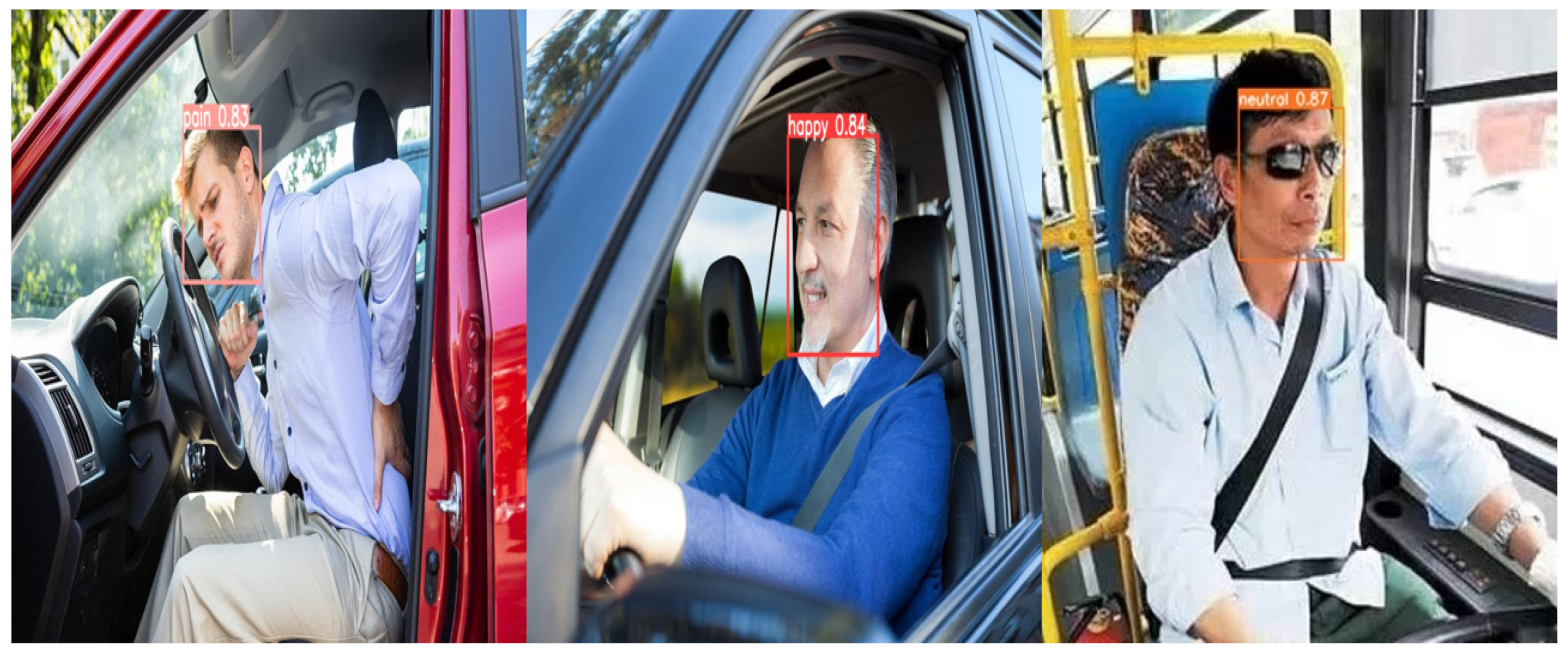
First, in response to the current scarcity of publicly available datasets for facial expressions of pain and distress, we created our own dataset. This dataset primarily includes three categories of expressions that drivers commonly exhibit during driving: happiness, neutrality, and pain. In the driving context, expressions of happiness and pain can influence certain driving decisions, and in this paper, these two types of expressions are classified as abnormal driving expressions.

(2)

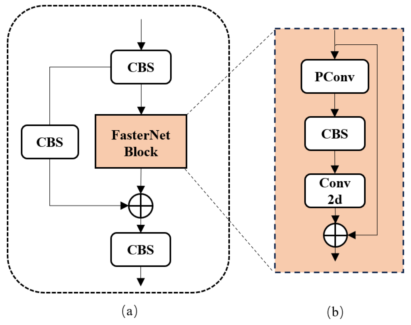
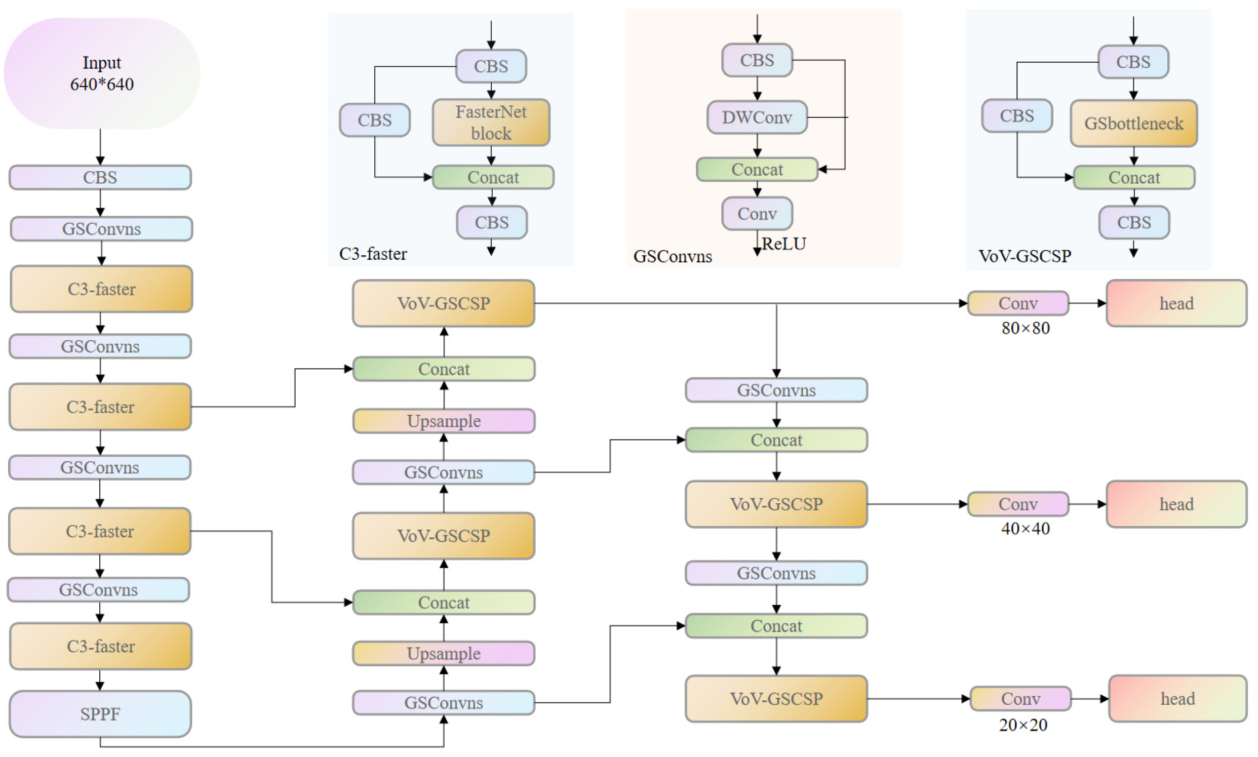
Next, in the realm of model lightweighting enhancements, a lightweight design approach was implemented for the YOLOv5 backbone network. This involved substituting the C3 module in the backbone network with the C3-faster module and replacing certain convolutional modules in the YOLOv5 network with the refined GSConvns lightweight module. Additionally, lightweight processing was applied to the neck network using the VoV-GSCSP module. These modifications were aimed at reducing the overall model’s parameter count, computational load, and size while ensuring that the model maintains a high level of detection accuracy.

(3)

Finally, pruning and fine-tuning the improved network model further reduced its parameter count, computational load, and size. Through fine-tuning, any performance loss incurred during pruning was compensated for, enabling the model to maintain a high level of detection accuracy and meet the practical detection needs in driving environments.

2. Introduction to the YOLOv5 Algorithm

YOLO (you only look once) [15] is an object detection algorithm, which implies that the neural network only needs to examine an image once to output results. In June 2020, the Ultralytics team introduced the YOLOv5 model as part of the YOLO series, and it has been continuously updated since then. YOLOv5 consists of five versions: YOLOv5n, YOLOv5s, YOLOv5m, YOLOv5l, and YOLOv5x. The only difference lies in the depth and width of the models, denoted as depth multiple and width multiple, respectively. These values increase in sequence from small to large, indicating a continuous increase in the model’s depth and width. For a comprehensive consideration of detection accuracy, model size, and detection speed, this method employs YOLOv5s as the baseline model for detection tasks. The YOLOv5s network structure consists of three main parts: the backbone network, the neck network, and the prediction end. The input end employs preprocessing techniques such as Mosaic data augmentation, adaptive anchor box calculation, and adaptive image scaling. Mosaic data augmentation involves random scaling, cropping, and arranging of images, enhancing dataset diversity and the ability to detect small objects. Adaptive anchor box calculation computes the optimal anchor box values for different datasets. Adaptive image scaling adds minimal black borders adaptively to the original image, reducing computational load and improving detection speed. The backbone network structure includes C3, CBS, and SPPF modules. The C3 module consists of three CBS convolutional layers and multiple bottleneck modules. The CBS structure combines Conv, BN, and SiLU activation functions. The SPPF module transforms feature maps of any size into a fixed-size feature vector, enhancing feature map expression capability. The neck network adopts feature pyramid network [16] and path aggregation network [17] structures as the feature fusion part of the network. The prediction end has detection heads for large, medium, and small objects with sizes of 20 × 20, 40 × 40, and 80 × 80, respectively. Multiple-scale predictions are made on the feature maps extracted from the neck network, ultimately providing bounding box, class, and confidence information for the detected objects.

3. Related Improvements

3.1. Backbone Network Improvement

In order to achieve model lightweighting while ensuring a certain level of accuracy, improvements were made to the backbone network of the model. In this study, the lightweight FasterNet [18] was integrated with the YOLOv5 backbone network’s C3 module. The FasterNet Block from the FasterNet network was employed to replace the bottleneck module in the C3 module, which significantly impacts the overall model’s computational and parameter count. While retaining the fundamental structure of the C3 module, the C3-faster module is formed. The C3-faster module was used to replace the C3 module in the backbone network responsible for feature extraction. The structure of the C3-faster module is illustrated in Figure 1. The CBS module is a convolutional module defined in the YOLOv5 network, consisting of a two-dimensional convolutional layer, a batch normalization layer, and a SiLU activation function. Through subsequent ablation experiments, it can be observed that compared to the original C3 module, the C3-faster module effectively reduces model parameters, computational load, and model size.

Figure 1. (a) C3-faster module structure; (b) FasterNet Block module structure.

The FasterNet Block consists of a partial convolution layer [18] (PConv), a CBS module, and a 2D convolutional layer. The inclusion of a BN layer within the CBS module accelerates model training and convergence speed. Additionally, the SiLU activation function introduces non-linear characteristics to the model, enhancing its expressive capacity. The partial convolution layer, denoted as PConv, selectively applies regular convolution to a subset of input channels for spatial feature extraction. It has no impact on other channels, keeping their sizes unchanged. This effectively reduces computational redundancy. The computational formulas for PConv and standard convolution are provided in Equations (1) and (2).

$$FLOP{s}_p=h\times w\times k^2\times c_p^2$$

(1)

$$FLOP\mathrm{s}=h\times w\times k^2\times c^2$$

(2)

Here, $h$, $w$, and $c$ represent the height, width, and number of channels, respectively, while k denotes the filter. $c_p$ represents the channels in the PConv network. When $c_p$/$c$ = 1/4, the computational cost of PConv is only 1/16th of that of standard convolution. Following PConv, to enhance model stability, training speed, and performance, input data normalization and SiLU activation functions are applied between the two standard convolution layers. This aims to boost the expressive power and training efficiency of the model. The FasterNet Block utilizes partial convolution to process input feature maps, reducing computational complexity and model parameters to enhance algorithm efficiency. This design enables a more effective utilization of computational resources, leading to accelerated model inference speed.

3.2. GSConv Module Improvement

The Ghost Conv [19] module is a high-performance convolutional module proposed by Han K and others. It addresses the issues of parameter accumulation and feature redundancy that arise when using a large number of standard convolutions for image feature extraction. The Ghost Conv module performs a small number of convolutions and linear transformation operations separately in its process, ultimately concatenating the feature maps obtained from these operations. Due to the outstanding performance of Ghost Conv, it has been widely used in research on lightweighting computer vision models since its introduction. However, there is a potential issue of information loss in the linear transformation. To address this problem, Li H and others proposed the GSConv module [20]. In the GSConv module, assuming the input channel number is C1 and the output channel number is C2, it first undergoes a standard convolution, reducing the channel number to C2/2. Subsequently, it passes through a depthwise separable convolution [21] (DWConv) with the channel number remaining unchanged. The feature maps from the two convolutions are then concatenated, followed by a shuffle operation.

The traditional depthwise separable convolution employs separate convolution channels, reducing both computational and parameter costs. However, it also leads to the loss of feature information, thereby diminishing feature extraction capability. The structure is illustrated in Figure 2, and the depthwise separable convolution primarily consists of two processes: depthwise convolution and pointwise convolution. It can replace convolution operations in a convolutional neural network, resulting in reduced parameter and computational costs. The computational formula for standard convolution is given by Equation (3), while the computational formula for depthwise separable convolution is provided in Equation (4). Here, $W$ and $H$ are the width and height of the input feature map, $K$ is the kernel size, and $C_1$ and $C_2$ represent the input and output feature channel numbers. Compared to standard convolution, the computational cost of depthwise separable convolution is reduced, as shown in Equation (5).

$$GFLOPs=W\times H\times K\times K\times C_1\times C_2$$

(3)

$$GFLOP{s}_1=W\times H\times K\times K{\times C}_1+W\times H\times 1\times 1\times C_1\times C_2$$

(4)

$$\frac{GFLOP{s}_1}{GFLOPs}=\frac{W\times H\times K\times K{\times C}_1+W\times H\times 1\times 1\times C_1\times C_2}{W\times H\times K\times K\times C_1\times C_2}=\frac{1}{K^2}+\frac{1}{C_2}$$

(5)

Figure 2. Depthwise separable convolution process diagram.

To address the limitations in the feature extraction capability of depthwise separable convolution, the GSConv module compensates by concatenating the feature maps from standard convolution with those from depthwise separable convolution. Subsequently, a shuffle operation is applied to the concatenated feature maps. This shuffle operation uniformly mixes and disrupts the channel feature information from depthwise separable convolution and standard convolution, enhancing the extraction of semantic information. However, it is worth noting that this operation may be less friendly to certain mobile hardware devices with limited computational resources.

In response to the aforementioned issue, improvements are made based on the GSConv module. A standard 2D convolution module and ReLU activation function were employed to replace the original shuffle operation, which consumes significant computational resources. This resulted in the formation of the GSConvns module, as illustrated in Figure 3. Convolutional operations are applied to the concatenated feature maps, followed by the application of the ReLU activation function. In terms of improvements, replacing the original shuffle operation with convolutional layers effectively reduces computational load while enhancing the model’s feature extraction capabilities. This modification also enables the model to be effectively implemented on some low-power mobile devices. After passing through the convolutional layers, the addition of the ReLU activation function introduces non-linearity, enabling the network to learn and represent more complex functions. This aids in reducing overfitting and improving the model’s generalization capabilities. The improvements contribute to enhancing the model’s feature representation, reducing model parameters and computational load, and increasing compatibility with hardware such as in-vehicle computers.

Figure 3. GSConvns module structure.

3.3. Improvement of the Neck Network

While lightweighting the model, it is essential to ensure the detection accuracy to meet practical requirements. In the neck network, a slim-neck structure was added based on the aforementioned GSConvns module. The slim-neck [18] structure includes the GSbottleneck module and the VoV-GSCSP module constructed based on the GSConvns module, where GSConvns is an improved lightweight convolution module in the YOLOv5 model, and VoV-GSCSP represents a lightweight module in the neck network of YOLOv5, as shown in Figure 4. Subsequently, the C3 module in the neck network was replaced with the VoV-GSCSP module containing GSConvns. Through experimental validation, this module, compared to the C3 module with a similar computational load, effectively improved the model’s detection accuracy, meeting the accuracy requirements in practical detection scenarios.

Figure 4. Slim-neck structure: (a) GSbottleneck module; (b) VoV-GSCSP module.

In this paper, the GSConvns module is used in the neck network and some parts of the backbone network to replace the regular CBS convolution module. This ensures a reduction in parameters, computational load, and model size, achieving lightweighting while also addressing the comprehensive extraction and fusion of target feature information. Furthermore, the introduction of the VoV-GSCSP module replaces the C3 module in the neck network, which was limited in terms of feature fusion. This not only reduces model complexity but also enhances model accuracy and inference time. The improved network model is illustrated in Figure 5.

Figure 5. Improved model structure.

3.4. Model Channel Pruning and Fine-Tuning

In the development of convolutional neural networks, there has been continuous improvement in both detection accuracy and speed. Some models exhibit stronger feature extraction capabilities, but this comes at the cost of increased computational resource consumption. Taking YOLOv5 as an example, in the YOLOv5 network model, multiple convolutional layers are used for feature extraction to enable accurate and fast object detection and localization. These layers output multiple channels, assigning corresponding weights to each channel for result prediction based on their magnitudes. However, some channel weight parameters are extremely close to zero, exerting minimal impact on the overall predictive capability of the network. Nevertheless, they still contribute to subsequent computation, leading to a certain degree of computational resource wastage and impacting detection efficiency. To address this, pruning operations [22] are applied to the improved model to eliminate redundant and non-critical weights. Before channel pruning, a scaling factor is introduced for each channel, which is multiplied by the output of that channel. Subsequently, the model undergoes sparse training to differentiate between different channels, facilitating better identification of redundant channels for the subsequent pruning operation. In the YOLOv5 network, there are multiple convolutional modules, and the batch normalization (BN) layer within these modules can accelerate network training convergence and enhance network generalization performance. The iterative process of batch normalization is as follows:

$${\mu }_B=\frac{1}{m}\sum _{i=1}^m{z}_i,$$

(6)

$${\sigma }_B=\frac{1}{m}\sum _{i=1}^m{(z_i-{\mu }_B)}^2,$$

(7)

where ${\mu }_B$ and ${\sigma }_B$ represent the mean and standard deviation computed for the input, $m$ is the current mini-batch size, and ε is a regularization parameter introduced to prevent standard deviation from becoming zero. Normalization is performed to obtain $\widehat{Z}$, and the input is reconstructed to obtain $Z_{out}$. The calculation formulae are shown in Equations (8) and (9).

$$\widehat{Z}=\frac{Z_{in}-{\mu }_B}{\sqrt{{\sigma }_B^2+\epsilon }}$$

(8)

$$Z_{out}=\gamma \widehat{Z}+\beta$$

(9)

Adding L1-norm regularization to the loss function can leverage the sparsity effect of the L1-norm to induce sparsity in the scaling factors of channels. The loss function for sparse training is represented as shown in Equation (10).

$$L=\sum _{(x,y)}l(f\left(x,W\right),y)+\lambda \sum _{\gamma ϵ\Gamma }g\left(\gamma \right)$$

(10)

In the equation, $(x,y)$ represents the training input and output. The first term represents the loss function for regular training, where $W$ is the training weight. The second term denotes the L1-norm regularization term used to induce sparsity. $\gamma$ is the scaling factor, $\Gamma$ represents the set of pruned channels, and $\lambda$ is the penalty factor.

During sparse training, the sparsity level of the model can be controlled and adjusted by a penalty factor. As the penalty factor is tuned, some channels in the batch normalization layer tend towards zero scaling factors. The outputs of these BN layers with very small scaling factors are also very small, having minimal impact on the overall predictive performance of the model while still consuming computational resources. Hence, these redundant channels are pruned, which may result in a slight loss in accuracy, but this loss can potentially be compensated for during the subsequent fine-tuning process. After sparse training, a pruning threshold is determined based on the specified pruning rate, and BN layer channels below this threshold are pruned from the network model. The pruning process is illustrated in Figure 6, where the blue and green rectangles, respectively, represent portions of the BN layer channels with different scaling factors after sparse training.

Figure 6. Model pruning process.

Fine-tuning is conducted to compensate for the loss in the original model’s expressive power caused by channel pruning. Channel pruning may introduce varying degrees of changes to the original network structure, leading to a decrease in model performance, particularly in terms of reduced detection accuracy. Therefore, fine-tuning helps improve the model’s accuracy to some extent, thereby restoring its performance.

4. Experimental Results

4.1. Introduction to the Experimental Dataset

Due to the scarcity of publicly available datasets for facial expressions of pain, the dataset used in this experiment is a self-made dataset. This dataset includes three types of facial expressions commonly observed during driving, namely, happy, neutral, and pain, with some of the painful facial expression images sourced from the PEMF dataset [23]. The dataset was first subjected to preprocessing steps such as uniform sample distribution and data augmentation. Subsequently, the LabelImg tool software is used to annotate the dataset in a format suitable for YOLO network training. The processed dataset comprises approximately 2500 images. The created dataset was divided into training, validation, and test sets in a ratio of 8:1:1. During the input stage of the YOLOv5 network, the model utilizes Mosaic data augmentation, involving the scaling and juxtaposition of any four images. This approach enriched the dataset and enhanced the network’s robustness to a certain extent.

4.2. Experimental Environment

The main configuration for the experiment includes a GPU, specifically the NVIDIA GeForce RTX 3090 and the PyTorch deep learning framework. During the training phase, the number of epochs was set to 400, the batch size was set to 32, and the optimizer chosen was SGD. The baseline model is YOLOv5s, with network depth gain and convolution channel gain parameters set to 0.33 and 0.5, respectively.

4.3. Evaluation Metrics

In this experiment, lightweighting of the model is pursued, and the evaluation metrics include the model’s parameter count (parameters), computational complexity (floating point operations, FLOPs), single object detection average precision (AP), mean average precision (mAP), and model size. The calculation process for mean average precision (mAP) is outlined as follows:

$$P=\frac{TP}{TP+FP,}$$

(11)

$$R=\frac{TP}{TP+FN,}$$

(12)

$$AP={\int }_0^{1}P\left(R\right)dR,$$

(13)

$$mAP=\frac{{\sum }_{i=1}^{n}A{P}_i}{n}.$$

(14)

Among these, $P$ stands for precision, indicating the proportion of correctly predicted samples among positive samples, while $R$ represents recall, denoting the proportion of positive samples predicted as positive among all positive samples. $TP$ signifies the number of true positive predictions (actual positives predicted as positives), $FP$ is the count of false positive predictions (actual negatives predicted as positives), and $FN$ is the number of false negative predictions (actual positives predicted as negatives). $AP$ represents the average precision value, $A{P}_i$ represents the average precision value for the corresponding category, $n$ represents the number of categories, $mAP$ is the mean average precision across all classes, and mAP@0.5 denotes the $mAP$ value when the IoU threshold is set to 0.5. Model size indicates the size of the weight file obtained after training.

4.4. The Analysis of Experimental Results

In the above dataset, facial expressions are mainly divided into three categories: happy, neutral, and pain. Ensuring the dataset and related parameters are the same, we selected several key lightweight networks for comparative testing, as shown in Table 1. It can be observed that compared to YOLOv7-tiny, the improved lightweight model exhibits a significant reduction in both parameter count and computational complexity. The mAP has increased by nearly two points, and there is also a noticeable decrease in model size. In comparison to MobileNet and ShuffleNet, two other lightweight networks, although there is a slight drawback in computational complexity, there are significant advantages in terms of parameter count, model size, and detection accuracy. Compared to the original model, there is a substantial decrease in parameter count, computational complexity, and model size. This makes the improved model more friendly to mobile devices with limited computational resources. While there is a slight decrease in detection accuracy by 1.2%, it still maintains a relatively high level of accuracy, achieving practical detection effectiveness in real-world usage.

Table 1. Comparative experiment.

Method	Parameters/M	FLOPs/G	mAP@0.5/%	Size/MB
YOLOv5s	6.7	15.8	85.7	13.7
YOLOV7-tiny	5.9	13.9	82.3	11.7
Mobilenetv3	5.5	2.8	83.1	17.9
Shufflenetv2	3.5	2.5	82.6	9.83
Improved YOLOv5	2.1	5.1	84.5	4.6

The ablation experiment, as shown in Table 2, indicates that the original model had a detection accuracy of 85.7%. After undergoing lightweight network model improvements, the detection accuracy experienced a slight decrease, reaching 84.9%. However, there was a noticeable reduction in computational load, parameters, and model size. Subsequently, pruning was applied to the lightweight improved model, resulting in further reductions in the above-mentioned metrics, while the detection accuracy decreased by only 0.4%, reaching 84.5%. Specifically, the detection accuracies for the three categories of facial expressions—happy, neutral, and pain—were 81.9%, 88.1%, and 83.5%, respectively; the model still maintains a robust detection performance in practical detection tasks. This satisfies the requirements for both practicality and accuracy, making it more suitable for deployment on mobile devices.

Table 2. Ablation experiment.

C3-Faster	GSConvns	VoV-GSCSP	Prune	Parameters/M	FLOPs/G	mAP@0.5/%	Size/MB
-	-	-	-	6.7	15.8	85.7	13.7
√	-	-	-	6.3	13.8	84.5	12.4
-	√	-	-	6.2	12.4	82.0	12.2
-	-	√	-	7.7	15.8	86.0	15.2
-	√	√	-	6.3	14.5	85.3	12.4
√	√	√	-	5.5	10.4	84.9	10.7
√	√	√	√	2.1	5.1	84.5	4.6

After adding the C3-faster module and GSConvns module, there was a reduction in model parameters, computational load, and model size. However, this led to a certain degree of accuracy decrease. The introduction of the VoV-GSCSP module helped compensate for some of the lost accuracy. Following these improvements, with reductions in model parameters, computational load, and model size, the mean average precision only decreased by 0.8%. After fine-tuning the pruned model, a mere 0.4% accuracy loss was observed, achieving reductions in the other three metrics. This indicates a nearly lossless pruning of the model to the maximum extent possible.

For a more intuitive assessment of the model’s real-world scene detection performance, the detection results are visualized, as depicted in Figure 7. The results encompass detections for driver expressions of pain, happiness, and neutrality. By conducting detection on images from actual driving scenarios beyond the dataset, it becomes evident that the method proposed in this paper demonstrates both accuracy and practicality. It is well-suited to meet the detection requirements in real-world scenes.

Figure 7. Detection results.

5. Conclusions

Considering practical application needs, this paper proposes an improved lightweight YOLOv5 detection model for detecting abnormal expressions in drivers during the driving process, potentially caused by body pain or discomfort. These abnormal expressions can influence driving behavior decisions. Timely detection of such expressions allows for intervention through the vehicle’s advanced driver-assistance system, preventing subsequent traffic safety incidents resulting from the driver’s discomfort. The experimental results indicate that the proposed improvement method, compared to the baseline model YOLOv5s, reduces the model size from 13.7 MB to 4.6 MB, an approximately 66.42% reduction. The parameter count has been reduced from 6.7 million to 2.1 million, and the computational load has been reduced from 15.8 billion to 5.1 billion. The improved model still maintains a high level of detection accuracy. Due to the reduction in computational load, parameter count, and model size, it can execute model inference and data processing more quickly. This not only enhances system response time but also reduces energy consumption. It is more convenient for deployment on mobile devices and contributes to the efficient operation of in-vehicle computers. In addition, in further research on lightweighting, it is essential to consider multi-angle recognition of the driver’s facial expressions as well as facial expression detection when the driver is in complex background environments. This includes scenarios with poor lighting conditions or high interference in the background.

References

1. Luo, Y.; Wu, C.-M.; Zhang, Y. Facial expression recognition based on fusion feature of PCA and LBP with SVM. Opt.-Int. J. Light Electron. Opt. 2013, 124, 2767–2770. [Google Scholar] [CrossRef]
2. Shan, C.; Gong, S.; McOwan, P.W. Facial expression recognition based on local binary patterns: A comprehensive study. Image Vis. Comput. 2009, 27, 803–816. [Google Scholar] [CrossRef]
3. Kumar, P.; Happy, S.; Routray, A. A real-time robust facial expression recognition system using HOG features. In Proceedings of the 2016 International Conference on Computing, Analytics and Security Trends (CAST), Pune, India, 19–21 December 2016; pp. 289–293. [Google Scholar]
4. Wang, X.; Jin, C.; Liu, W.; Hu, M.; Xu, L.; Ren, F. Feature fusion of HOG and WLD for facial expression recognition. In Proceedings of the 2013 IEEE/SICE International Symposium on System Integration, Kobe, Japan, 15–17 December 2013; pp. 227–232. [Google Scholar]
5. Bartlett, M.S.; Littlewort, G.; Frank, M.; Lainscsek, C.; Fasel, I.; Movellan, J. Fully automatic facial action recognition in spontaneous behavior. In Proceedings of the 7th International Conference on Automatic Face and Gesture Recognition (FGR06), Southampton, UK, 10–12 April 2006; pp. 223–230. [Google Scholar]
6. Anderson, K.; McOwan, P.W. A real-time automated system for the recognition of human facial expressions. IEEE Trans. Syst. Man Cybern. Part B Cybern. 2006, 36, 96–105. [Google Scholar] [CrossRef] [PubMed]
7. Pantic, M.; Patras, I. Dynamics of facial expression: Recognition of facial actions and their temporal segments from face profile image sequences. IEEE Trans. Syst. Man Cybern. Part B Cybern. 2006, 36, 433–449. [Google Scholar] [CrossRef] [PubMed]
8. Li, J.; Jin, K.; Zhou, D.; Kubota, N.; Ju, Z. Attention mechanism-based CNN for facial expression recognition. Neurocomputing 2020, 411, 340–350. [Google Scholar] [CrossRef]
9. Shan, K.; Guo, J.; You, W.; Lu, D.; Bie, R. Automatic facial expression recognition based on a deep convolutional-neural-network structure. In Proceedings of the 2017 IEEE 15th International Conference on Software Engineering Research, Management and Applications (SERA), London, UK, 7–9 June 2017; pp. 123–128. [Google Scholar]
10. Li, J.; Zhang, D.; Zhang, J.; Zhang, J.; Li, T.; Xia, Y.; Yan, Q.; Xun, L. Facial expression recognition with faster R-CNN. Procedia Comput. Sci. 2017, 107, 135–140. [Google Scholar] [CrossRef]
11. Febrian, R.; Halim, B.M.; Christina, M.; Ramdhan, D.; Chowanda, A. Facial expression recognition using bidirectional LSTM-CNN. Procedia Comput. Sci. 2023, 216, 39–47. [Google Scholar] [CrossRef]
12. Wang, S.; Cheng, Z.; Deng, X.; Chang, L.; Duan, F.; Lu, K. Leveraging 3D blendshape for facial expression recognition using CNN. Sci. China Inf. Sci. 2020, 63, 120114. [Google Scholar] [CrossRef]
13. Li, J.; Li, M. Research on facial expression recognition based on improved multi-scale convolutional neural networks. J. Chongqing Univ. Posts Telecommun. 2022, 34, 201–207. [Google Scholar]
14. Qiao, G.; Hou, S.; Liu, Y. Facial expression recognition algorithm based on combination of improved convolutional neural network and support vector machine. J. Comput. Appl. 2022, 42, 1253–1259. [Google Scholar]
15. Redmon, J.; Divvala, S.; Girshick, R.; Farhadi, A. You only look once: Unified, real-time object detection. In Proceedings of the IEEE Conference on Computer Vision and Pattern Recognition, Las Vegas, NV, USA, 27–30 June 2016; pp. 779–788. [Google Scholar]
16. Lin, T.-Y.; Dollár, P.; Girshick, R.; He, K.; Hariharan, B.; Belongie, S. Feature pyramid networks for object detection. In Proceedings of the IEEE Conference on Computer Vision and Pattern Recognition, Honolulu, HI, USA, 21–26 July 2017; pp. 2117–2125. [Google Scholar]
17. Liu, S.; Qi, L.; Qin, H.; Shi, J.; Jia, J. Path aggregation network for instance segmentation. In Proceedings of the IEEE conference on Computer Vision and Pattern Recognition, Salt Lake City, UT, USA, 18–23 June 2018; pp. 8759–8768. [Google Scholar]
18. Chen, J.; Kao, S.-h.; He, H.; Zhuo, W.; Wen, S.; Lee, C.-H.; Chan, S.-H.G. Run, Don’t Walk: Chasing Higher FLOPS for Faster Neural Networks. In Proceedings of the IEEE/CVF Conference on Computer Vision and Pattern Recognition, Vancouver, BC, Canada, 17–24 June 2023; pp. 12021–12031. [Google Scholar]
19. Han, K.; Wang, Y.; Tian, Q.; Guo, J.; Xu, C.; Xu, C. Ghostnet: More features from cheap operations. In Proceedings of the IEEE/CVF Conference on Computer Vision and Pattern Recognition, Seattle, WA, USA, 13–19 June 2020; pp. 1580–1589. [Google Scholar]
20. Li, H.; Li, J.; Wei, H.; Liu, Z.; Zhan, Z.; Ren, Q. Slim-neck by GSConv: A better design paradigm of detector architectures for autonomous vehicles. arXiv 2022, arXiv:2206.02424. [Google Scholar]
21. Howard, A.G.; Zhu, M.; Chen, B.; Kalenichenko, D.; Wang, W.; Weyand, T.; Andreetto, M.; Adam, H. Mobilenets: Efficient convolutional neural networks for mobile vision applications. arXiv 2017, arXiv:1704.04861. [Google Scholar]
22. Liu, Z.; Li, J.; Shen, Z.; Huang, G.; Yan, S.; Zhang, C. Learning efficient convolutional networks through network slimming. In Proceedings of the IEEE International Conference on Computer Vision, Venice, Italy, 22–29 October 2017; pp. 2736–2744. [Google Scholar]
23. Fernandes-Magalhaes, R.; Carpio, A.; Ferrera, D.; Van Ryckeghem, D.; Peláez, I.; Barjola, P.; De Lahoz, M.E.; Martín-Buro, M.C.; Hinojosa, J.A.; Van Damme, S. Pain E-motion Faces Database (PEMF): Pain-related micro-clips for emotion research. Behav. Res. Methods 2023, 55, 3831–3844. [Google Scholar] [CrossRef] [PubMed]