Abstract
In light of the energy crisis, extensive research is being conducted to enhance load forecasting, optimize the targeting of demand response programs, and advise building occupants on actions to enhance energy performance. Cluster analysis is increasingly applied to usage data across all consumer types. More accurate consumer identification translates to improved resource planning. In the context of Industry 4.0, where comprehensive data are collected across various domains, we propose using existing sensor data from household appliances to extract the usage patterns and characterize the resource demands of consumers from residential households. We propose a general pipeline for extracting features from raw sensor data alongside global features for clustering device usages and classifying them based on extracted time series. We applied the proposed method to real data from three different types of household devices. We propose a strategy to identify the number of existent clusters in real data. We employed the label data obtained from clustering for the classification of consumers based on data recorded on different time ranges and achieved an increase in accuracy of up to 15% when we expanded the time range for the recorded data on the entire dataset, obtaining an accuracy of over 99.89%. We further explore the data meta-features for a minimal dataset by examining the necessary time interval for the recorded data, dataset dimensions, and the feature set. This analysis aims to achieve an effective trade-off between time and performance.
1. Introduction
Industry 4.0 transforms various aspects of industry and everyday life by integrating digital technologies. As a result, there is a massive quantity of data from a multitude of sources, which creates both a challenge and an opportunity for businesses and individuals alike. One area where this data revolution is pronounced is in the context of household appliances. These appliances, which have become increasingly sophisticated, now generate a vast amount of usage data that can be harnessed to gain valuable insights.
The term “big data” has become synonymous with this massive volume of data, which has a complex and varied nature. Intelligent appliances are equipped with sensors, connectivity features, and innovative functionalities that allow them to collect data on operational efficiency and usage patterns. These data can unveil a treasure trove of information that can be used to reduce energy consumption, optimize appliance performance, and even predict maintenance needs when properly collected and analyzed.
Collecting these data does not require any additional effort from the user. Once collected, it can offer insights into usage habits and preferences, energy efficiency, and appliance functionality [1,2]. Manufacturers can provide a more personalized user experience, improve overall energy consumption, and estimate future usage patterns with the help of advanced data analytics and machine learning.
In the context of the energy crisis, an important applicable research topic concerns the optimizing of resources. Understanding consumer behavior and estimating future needs could improve load forecasting and enhance targeting of the demand response. This would positively impact both distribution and supply services. Moreover, it is possible to recommend cost-effective utilization that would benefit end consumers.
Grouping consumers into large categories such as industry, commercial, and residential does not provide enough granularity. This is due to marked differences between consumers with similar characteristics. A rigorous evaluation of the profiles of the users from each class is needed.
The most significant percentage of the final electricity consumption for many countries [3] is due to residential consumers. Home appliance usage is a major component of the total energy consumption of a residence [4,5,6]. Appliance usage depends on multiple factors, which causes heterogeneity in the household sector that cannot be reflected in a single profile that includes all appliances. Consequently, multiple usage profiles should be explored to improve the understanding of the household sector. Identifying categories of usages for appliances and usage patterns leads to better characterization of residences from the consumption perspective. Additionally, it can be employed to offer feedback, suggesting suitable actions for occupants to improve the energy performance of a building. Thus, this is the motivation behind our work. Therefore, this paper aims to provide a method for identifying consumer behavior in appliance usage based on data recorded by sensors attached to devices.
Sensor-generated raw data can serve purposes beyond their initial intent. One of the most used data types for sensor-recorded data is time series. Due to the high dimensionality of time series data, processing it with automated algorithms can be tedious, if possible. Another challenging aspect is comparing time series of varying lengths for classification purposes. For this reason, feature-based representation of data should be used to measure the similarity between pairs of time series [7]. Furthermore, time series data can be leveraged to extract features independent of the time domain, which can later be utilized in various processing tasks such as clustering [8]. A particular application of features extracted from time series sensor data implies identifying running cycles [9] and further processing them to compute features.
Many factors influence machine learning performance, each playing a crucial role in shaping the efficacy of models and algorithms. Pivotal factors include the quality and quantity of the training data. An equally significant factor is the choice of the features extracted from the data used for training, as relevant and discriminative features contribute to the model’s ability to discern patterns within the data. The dataset’s complexity and size, the chosen algorithm’s intricacies, and the desired level of model accuracy collectively contribute to the time versus performance trade-off. Thus, another objective of our work is to identify these factors and showcase their impact on the task of usage characterization.
In our work, we present an original method for extracting and computing features from raw sensor data to group and identify consumer behavior. As a proof of concept, our general pipeline is applied to data obtained from real-world appliance utilization. We transform the raw input data into the time series of interest and then compute a subset of their features. Our computed features-driven clustering strategy allows us to identify the specific usage categories present in a given dataset. The clustering strategy gives us labels for the data, which are further employed as training data to build models in a supervised learning strategy. To our knowledge, no similar pipeline exists for identifying the household appliances consumer class from raw sensor data that records device functioning information. We identify the context-relevant dimensions for the prediction task, including the recorded time interval, the training data size, and the feature set, and we illustrate their impact from a performance perspective. We summarize the main contributions of our work as follows:
- pipeline for consumer behavior identification
- feature extraction and computation for labeling assignment
- identification of context-relevant dimensions for prediction
This paper is structured as follows: In Section 2, we present the related work on feature extraction from time series, clustering, and classification with an accent on state-of-the-art residential consumer estimation and grouping, as well as the metrics that can be used to evaluate the results. We proceed with the pipeline and algorithms proposal for consumer class extraction alongside a set of features that can be used in Section 3. We apply our method in Section 4 to actual household data, where we investigate three main dimensions to determine the minimal requirements for an appliance dataset and finish with some concluding remarks.
2. Related Work
2.1. Time Series
Time series data is the prevailing data type utilized in various domains [10]. It refers to a sequence of observations x recorded at specific time instances t, where t belongs to a predetermined set of times T.
Some examples of time series are data recorded from the sensors of different devices, the energy and water consumption recorded during a period of time, or the duration an appliance is used per day. Intermittent time series are a particular kind of time series. This term refers to those series with zero values on multiple entries without obvious patterns of variation [11]. An example of intermittent time series is the usage time series of appliances. Due to the fact that appliances are not used constantly, multiple zero values can appear depending on the granularity level of data, which means that the appliance was not used in a given time interval.
Feature representations can be used to measure the similarity between pairs of time series. This is useful for tasks such as classification, clustering, or extracting knowledge from data [12]. Global features are designed to capture patterns spanning the entire time series. Data are translated from a complex temporal dimension into a more concise and quantifiable representation by computing and extracting these global patterns. Additionally, this approach facilitates the comparison of different time series that may have varying data dimensions [7].
Some patterns can be identified depending on the source of the time series and the context in which the data are recorded. For example, in the case of sensors that record functioning information from devices, there can be different patterns based on the devices’ usage cycles. Detecting running cycles (which can be washing cycles in the case of washing machines, cooking cycles in the case of microwaves or ovens) from sensor data typically involves signal processing and analysis, and the approach may vary depending on the type of sensor and the specific application. In most methods, after data preprocessing, feature selection, and segmentation, a criterion or algorithm is defined to determine when a running cycle starts and ends based on the identified peaks or features. In previous work [9], we present a method for detecting cycles from raw data recorded from appliances based on a pair of start and stop markers from the data.
2.2. Cluster Analysis of Household Devices Usage
Applying cluster analysis of electrical consumers is the subject of multiple works [13,14,15]. Most of them use electrical measurements from an entire location. For example, in [16], an electricity consumer characterization framework is presented, where historical data regarding the measurements of local consumers from a distribution company are used.
Residential consumers constitute the largest share of total energy consumption [3]. Their usage patterns are influenced by multiple factors, including the number of individuals in a household, the prevailing lifestyle, and the presence of power-intensive appliances, as highlighted in Chicco’s overview of the subject [17]. Evaluating the determinants of household electricity consumption using cluster analysis was the subject of [18]. Using K-means and feature selection, four distinct groups were identified based on energy data specificities, such as the number of bedrooms, the number of rooms, the number of appliances in households, the billed energy consumption, and survey energy consumption.
Considering a household with m appliances and k operating modes, the total energy consumption at time n is defined in [19] as
In this equation, is the operating On/Off status of the i-th appliance in time n, which can be [0,1], is the electricity consumed in a particular operating mode, and denotes the measurement of background noise at time n.
The significance of household appliance usage extends beyond merely energy consumption. It profoundly affects both water and energy resource utilization within a residence [4,5]. Recognizing and effectively extracting these usage patterns leads to more accurate resource allocation. Also, it empowers households to make informed decisions about their consumption, which could help with more sustainable and efficient utilization of these vital resources. This knowledge is particularly essential in today’s world, where sustainability and responsible resource management are of great importance.
Extracting usage patterns from appliances in smart home appliances was performed in [20]. Two types of usage patterns are proposed: daily behavior-based and cluster-based statistical usage patterns.
Clustering techniques are used for partitioning a set of objects into groups to maximize the similarity between objects inside a group and minimize the similarity between clusters. One algorithm commonly used for clustering is K-means [21] due to its applicability to large datasets and its versatility. Before applying a clustering algorithm that is based on distance, such as K-means, the features should be normalized [22]. An example of normalization is removing the mean and scaling to unit variance.
Clustering becomes even more complex as the number of features increases [23]. Using entire time series data for tasks such as clustering implies high dimensionality of the data. Due to this reason, features are usually computed from the data. In the case of household electricity demand, features such as annual electricity usage, the standard deviation, or the size of peak demand are frequently used [24].
The elbow method [25] is a widely used technique in the field of cluster analysis, particularly in unsupervised machine learning, to determine the number of clusters revealed in a given dataset [26]. In practice, selecting the exact elbow point can be subjective, as it may not always be as clear-cut as a distinct elbow shape. However, the elbow method offers a valuable rule of thumb for determining the number of clusters that align with the data’s underlying structure and the analysis objectives.
When the ground truth is unknown, a more precise assessment of the number of clusters within a given range of potential cluster numbers can be performed by testing the results of various metrics across potential numbers of clusters. One example of such metrics is the Calinski–Harabasz index (also known as the variance ratio criterion), which represents the ratio of the sum of the between-clusters dispersion and the within-cluster dispersion for all clusters [27]. The range for the Calinski–Harabasz index is the interval [0, ∞], where a higher value indicates a better solution. Another method is the Davies–Bouldin index, which computes the average similarity between clusters. The similarity is a measure that compares the distance between clusters with the size of the clusters themselves [28]. The minimum Davies–Bouldin index score is 0, where a lower value indicates better clustering. The silhouette coefficient [29] considers both the mean distance between all other points in the next nearest cluster and a sample and the mean distance between a sample and all other points in the same class.
2.3. Appliance Classification
Classification is a fundamental and widely used task in machine learning, and it plays a crucial role in solving various real-world problems. The primary goal is to assign a label or category to a given input data point based on a set of features. There are several algorithms commonly used for multiclass prediction, such as K-nearest neighbors (KNN) [30], multiclass support vector machines (SVM) [31], random forest [32], and naive Bayes [33]. Another effective approach for addressing intricate classification tasks is the multilayer perceptron (MLP) [34], which belongs to the category of artificial neural networks.
Several works in load monitoring and appliance classification have sought to enhance the understanding of energy consumption patterns within households [35,36]. Some works use appliance data and have, for example, shown a positive impact of incentive payments in the context of electricity consumption and price incentives in a pilot test in Belgium when the flexibility of smart appliances was used [37]. In [38], extraction of consumption patterns at the appliance level in the context of demand-side management was undertaken. The work used load profiles and electricity consumption. One of the challenges that studies in the literature often encounter is the need for clean data on the actual power consumption of individual appliances or households, which may not always be accessible or available in practice [39]. Another challenge is the need for user activity data, along with both indoor and outdoor environmental condition data [40].
In response to these data limitations, alternative strategies to gain insights into appliance usage patterns could be used. One promising approach is to take advantage of the wealth of data generated by sensors embedded within modern appliances. These sensors provide valuable information about appliance operations, usage frequency, and potential anomalies. A sensor-driven methodology opens up new possibilities for appliance classification and load monitoring, making it a compelling area of research for those seeking more efficient and practical energy management and conservation solutions.
Household appliance usage exhibits distinctive patterns that tend to vary depending on the specific day of the week. This observation was proven in previous work [1], which highlighted the influence of our weekly routines and schedules on how we interact with our appliances. This correlation between daily routines and appliance usage patterns has significant implications for energy management, as it allows for optimizing energy consumption strategies that align with these trends. From the perspective of extracting global features from usage time series data, aligning the information regarding the day of the week and separating patterns based on this could further improve classification results.
3. Pipeline for Usage Characterization
3.1. Method for Consumer Behavior Identification
The usage of appliances represents a significant percentage of the resource consumption of a residential client. Enhancing our comprehension of these usage patterns enables more accurate load estimation and peak demand estimation of energy and water consumption due to improved demand-side management. This can be achieved by categorizing household appliances according to their usage patterns and using resource planning strategies specific to the usage class. We propose a method for determining usage class based on sensor data that have already been collected to reach this objective. Our method includes preprocessing data, extracting global features independent of the time domain from time series sensor data, labeling a training set through clustering, and subsequent prediction based on a reduced dataset. We illustrate the pipeline in Figure 1.
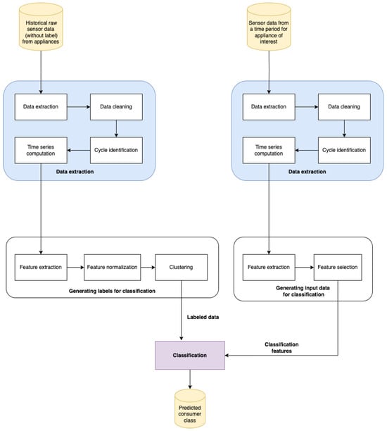
Figure 1.
Method for usage characterization of appliances from raw data.
Our system’s input consists of data recorded by sensors attached to devices that are automatically sent to a data lake system from which we can further process them. Our output is a predicted consumer class.
We structure the pipeline into main components based on their role in the system. The main components of our method are a data extraction module, a module for generating labels for classification, a module for generating input data for classification, and a classification module.
Regardless of the type of appliance, model, or manufacturer, data from an appliance contain information regarding its internal status and functioning, as well as signals triggered by external factors, such as network issues or changes made by the user. The essential components of a dataset include the type of the signals, the alphanumeric values, the timestamps it has recorded, and the timestamps it has received at the data warehouse. Depending on the type of the signal, it can be sent periodically, be event-based, or involve a combination of them. From our practical experience, we found it necessary to address at least the following complexities: large volume of data, duplicate values, missing data, variability in the dataset, and noise. Thus, we define this pipeline to address these complexities in the raw data.
In Table 1, we exemplify different types of complexities as follows:

Table 1.
Example of minimal data recorded from functioning devices.
- Duplicate data: the Name 1 signal from line 2 is a duplicate of line 1, the only difference between the two of them being the received timestamp
- Variability in data types: the Name 2 signal value type is an alphabetical one, while the values of the other signals are numerical values
- Variability in timezone: for the Name 3 signal, GMT +2 is used, while for the other signals, GMT +1. Different time zones can appear due to the geographical location of the devices. The usage of different time zones could imply the need for normalization before further processing of the data.
Handling the volume of data resulting from devices is a challenge before processing these data for any particular task. Due to its generality, our method can be applied regardless of the appliance type or if internal information about the data types and the device’s functioning is known or not.
Our data extraction module is composed of four components: identification of relevant data and extracting them, data cleaning, cycle identification, and time series computation. Due to the nature of the data (which can be classified as big data), the first appropriate step is extracting the usage data of interest to overcome the dataset dimensionality complexity. The next step is the semantical and syntactical cleaning of the raw data. In previous work [41], we introduced a comprehensive and versatile methodology tailored for the analysis and cleaning of data. This methodology offers insights and techniques that can be effectively adapted to address our study’s unique challenges and requirements.
Most appliances are used during a specific interval, which can be defined by the start of the device, its running to solve a task, and its stopping. For example, washing machines or dishwashers clean clothes or dishes, while an oven or a microwave cooks or heats food. We will refer to this sequence of events as a cycle. Our previous work [9] introduces a method for detecting cycles from raw data recorded from devices with running patterns similar to the ones described above. After the data are extracted and cleaned, an intermittent time series of interest can be composed of elements.
The pipeline’s final objective is to predict an appliance’s usage category. This requires pattern identification. A helpful tool is provided by statistics in the use of devices that can be extracted based on running patterns. High-dimensional data, such as time series recorded during different time intervals, are more challenging to compare and group based on their common patterns. One approach to address this challenge is to compute global features unrelated to the time domain, which would capture the patterns that span the entire signal duration, regardless of whether the data are recorded over a shorter or longer time span.
The features we select should identify the utilization patterns of the devices optimally. Daily device usage patterns exist in real data as identified in [1]. As we investigate appliance usage, we expect some daily patterns to exist. Moreover, days might differ within weeks or months, so month granularity is important to extract. Therefore, we compute the average number of seconds a device is used per day on a weekday alongside the average number of cycles; the same features are also computed using a month as a time granularity unit.
The feature dimensions can have different ranges. As a consequence, feature normalization should be performed at this point; an appropriate approach is to remove the mean and scale the features to unit variance. Based on the computed data, a clustering algorithm is applied, which results in consumer class identification and grouping. The clustering output consists of labels, which are characteristics of each cluster identified from the data. The labels obtained from clustering, alongside the data, are used as training data for classification.
It is important to predict an appliance’s future usage as soon as possible so that the estimation has better precision as soon as the data are available. Given raw sensor data from a given time period for a particular appliance, we propose using the same data extraction steps. As a result, features are extracted and computed to classify an appliance based on that period. The output of the presented pipeline is the determination of the consumer usage class.
3.2. Algorithmic Representation
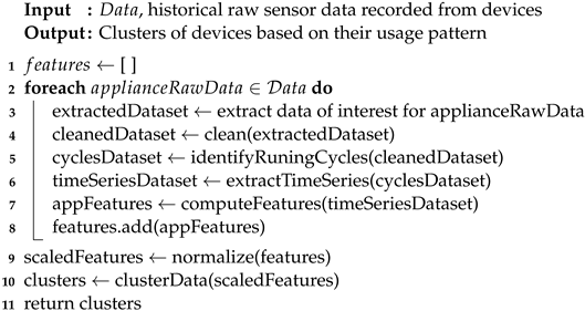
, the algorithm proposed for clustering devices, is presented in Algorithm 1. It takes the raw sensor data as input and returns the appliances grouped by their usage patterns. The output of the algorithm consists of pairs composed of data instances and labels. Starting from line 2, we process each of the appliances’ raw data separately. In line 3, data is first extracted to reduce the dimensions and then cleaned. In the step from line 5, we identify the running cycles, and then we construct time series data from them. In the step of the algorithm from line 7, features are extracted from the time series data that are independent of the time domain and can be extrapolated from a larger or more limited time span.
| Algorithm 1: DetectClustersFromRawData: Consumer class characterization from raw sensor data |
 |
The pairs obtained from Algorithm 1 are further used as training data for supervised learning. The complete algorithm used for the determination of the consumer class of an appliance is presented in Algorithm 2. The appliance data taken as a parameter represent the raw sensor data of the new appliance of interest for which we want to predict the future usage patterns. Due to the extraction of relevant features from time series data, the interval from which data are recorded before using them as input in Algorithm 2 can be different from the ones used for the training set. The algorithm’s output is the predicted class for the specific consumer corresponding to input.
In the steps from lines 1–4, the data of interest are extracted and cleaned, running cycles are identified, and time series data are extracted. The features used for classification are computed in line 5. In line 6, we use Algorithm 1 to receive the pairs of that are further used for training in line 8. The algorithm returns the class predicted for the input consumer.
Although the strategy was designed for a specific data source, the pipeline and algorithms presented above can be applied to data with other characteristics, such as different time ranges for the recorded data, different appliance particularities, or even different data sources.
| Algorithm 2: DetermineConsumerClass: consumer class determination from raw sensor data |
| Input : , historical raw sensor data recorded from devices , limited raw sensor data recorded for one device Output: Consumer class prediction for applianceData
|
For good quality of results, there has to be a trade-off between the desirable performance, the processing time, and the data available. More specifically, there is a trade-off between the performance obtained and the data available, as well as the data used and the processing time needed for that amount of data. Therefore, we define the achieved quality as a function of three dimensions: the time interval, the data size, and the feature set.
is the period when data is recorded from, refers to the amount of data used in the processing task, and refers to the features used for processing. We propose calibrating the three dimensions by maintaining two fixed dimensions while varying the third one.
Using raw time series data is unsuitable for clustering due to high dimensionality. This imposes the need to compute and extract features to characterize the data. The extracted features can illustrate the behavior of different time amounts depending on the ranges for the existing time series data. For example, the usage of day, week, month, three months, half a year, a year, and so on could be appropriate.
We propose a compact set of features that can be computed from usage information data by reducing the entire time series data to a couple of features that illustrate the usage in a higher period. More specifically, the average number of cycles per time and the average runtime for the same period are used.
In previous work [1], we showed that household appliance usage has a general pattern depending on the day of the week. We propose an extended set of features computed on both a global unit scale (with a more extensive time granularity) and separated based on weekdays to maintain the information regarding household appliance daily usage patterns. We found it beneficial to extract a set of 16 features to categorize the usage of household appliances, outlined as follows:
- Average number of cycles per higher time amount ⇒ one feature
- Average runtime per higher time amount ⇒ one feature
- Average runtime per each weekday ⇒ seven features
- Average number of cycles per each weekday ⇒ seven features
The advantage of these feature sets is the small amount of usage data needed to characterize the device patterns and their independence from the device type. The relevant time interval of the features might vary from small intervals, such as hours, to months or seasons.
4. Application on Household Data
4.1. Context and Dataset Description
Several types of high-consumer appliances have functioning cycles. These appliances are designed to operate through predetermined cycles that optimize their performance while minimizing energy consumption. Understanding usage patterns to better predict future usage contributes to energy efficiency, ultimately benefiting both households and the environment.
Our experiments processed data logs recorded from three different device types during one year. To maintain data anonymity while keeping data generality as our methodology fits any appliance, we will refer to the appliances from our experiments as appliance type 1, appliance type 2, and appliance type 3.
From the available data, we keep the relevant ones. This implies maintaining those devices with a statistically relevant number of running cycles and consistent running cycles. As such, we maintained the following data:
- cycles with a duration of more than 5 min or less than 12 h, since outside these time ranges, running cycles are not plausible for the device types used
- instances that have more than 20 running cycles per year, since these devices have statistical relevance due to the higher number of usages in one year
Table 2 presents the numerical dimensions of the used dataset. We have tens of thousands of devices with millions of running cycles recorded during one year for all device types. Altogether, we formed our dataset from around 100,000 different appliances in the three types.
Table 2.
Dataset sizes separated per appliance type.
On our cleaned dataset, after detecting the running cycles of each device, we used a time series unit of one day of usage and computed each device’s run time in seconds per day and the number of running cycles per day. The result, which we call the time series dataset, is formed from two univariate intermittent time series as follows:
- Runtime time series, where one point represents each device’s runtime in seconds per that day of the year.
- Cycles time series, where one point represents the number of cycles that the device was used for in a given day
Device classification becomes possible based on the usage patterns in the data. Our selected features could illustrate these patterns. We use two granularity levels for time amounts to compute these features: day and month. We computed each device’s average runtime in seconds and the number of running cycles. The resulting features are illustrated in Table 3.
Table 3.
Features extracted from time series usage data.
As features have different scales, we normalized the features by using a standard scaler. Afterward, we apply processing steps, such as clustering or classification.
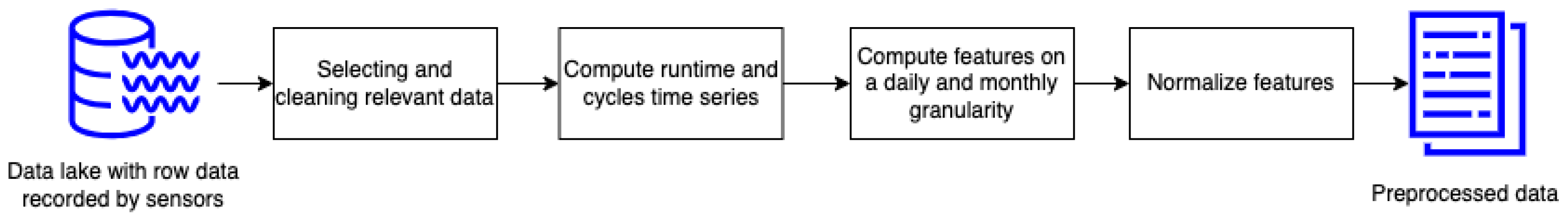
The steps presented above are summarized and organized in Figure 2. The input consists of raw sensor data from three types of devices, and the output is the normalized features that were computed for each appliance.

Figure 2.
Summary of the data preprocessing steps. The output of the steps is further used for clustering and classification experiments.
In our experiments, from the scikit-learn library [42], we used implementations of the standard scaler, K-means, and classification methods (K-neighbors classifier, random forest classifier, Gaussian naive Bayes, support vector machines, and multilayer perceptron).
4.2. Appliance Usage Clustering
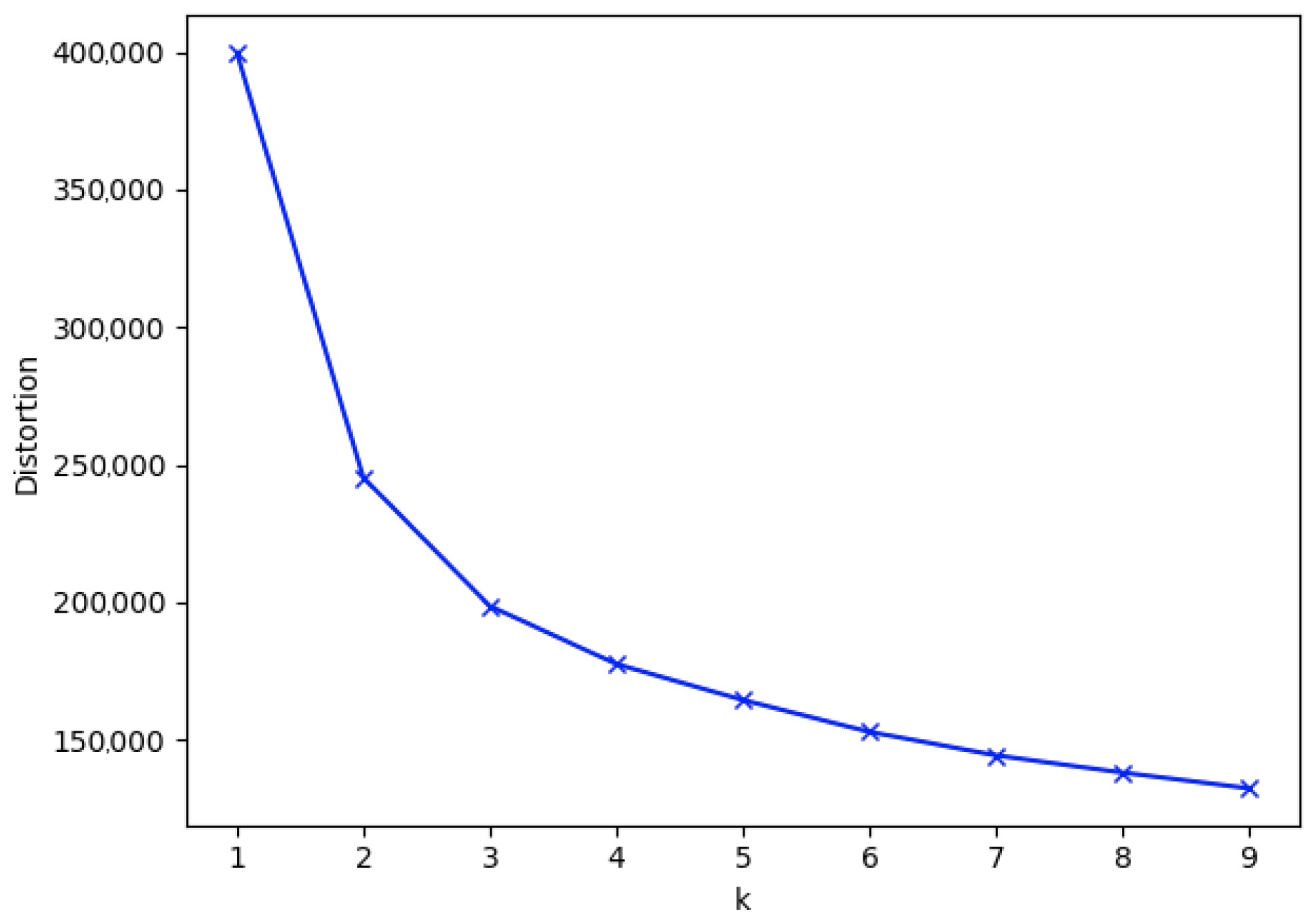
We apply the elbow method to find the number of clusters present in our data. Figure 3 presents the appliance type 1 data results, where we have the number of clusters on the OX axis and the distortion on the OY axis.

Figure 3.
Elbow method results for appliance type 1 data.
We use K-means for clustering due to its versatility and applicability to large datasets. The elbow method resulted in a number of clusters equal to 3, 4, or 5 being appropriate. We continue our analysis by computing the scores obtained by clustering where the number of clusters is variable in Table 4. We use the Calinski–Harabasz index, the Davies–Bouldin index, and the silhouette coefficient for evaluation.
Table 4.
Clustering evaluation score for appliance type 1 data.
The Calinski–Harabas index illustrates the variance of the between-clusters dispersion and the within-cluster dispersion. A higher Calinski–Harabasz score is achieved when the clusters are dense and well separated. From our results, the best variance, with a score of 28.903 for the index, was obtained for three classes. The Davies–Bouldin index measures cluster similarity, so a score closer to 0 is desirable. We obtained a score of 1.06 for the three classes.
Each metric suggests that there are three patterns in the data at hand. The results confirm the grouping of appliance usage into three classes based on their usage: low-used, medium-used, and highly used devices. We proceeded with the same experiments on all three device types. The usage behavior specifications scaled across all data samples, which proves that there is clear separation of devices.
We projected the data into a two-dimensional space to visualize the clustering results by selecting the most significant features. Figure 4 presents the data projection from appliance type 1 for k = 3. We have the average number of monthly cycles on the OX axis and the average runtime per month in seconds on the OY axis. One point represents one appliance, and the color of the point represents the class of that appliance after clustering.
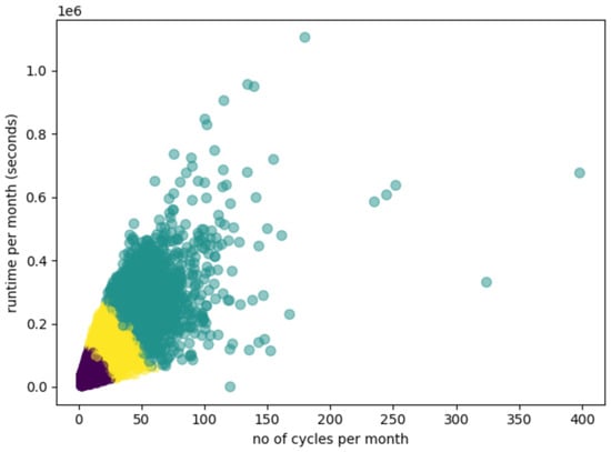
Figure 4.
Clustering results after applying a three classes K-means algorithm on appliance type 1 data. The color of the points represents the classes according to clustering.
Clear separation lines are visible for all of the classes of device type 1 which means using three clusters is appropriate. The outlier points from clusterization correspond to devices used on more than 80% of the days. For the other two appliance types, the evaluation revealed the same behavior: pattern grouping on three clusters, with quite clean separation and the presence of outliers, which are associated with the higher class of usage due to the high number of cycles per month and the increased number of seconds of runtime per month.
Looking at the number of instances from each class for appliance type 1, of a total of 40,773 appliances, 3118 (7.65%) have high usage, 13,575 (33.30%) are medium, and 24,080 (59.05%) have low usage. In the case of appliance type 2, we have 11,288 (69.25%) low-usage devices, 4297 (26.36%) average usage, and 755 (4.63 %) high-usage devices. From the appliance type 3 dataset, 32, 568 (81.82%) devices have low usage, 6302 (15.8%) devices have medium usage, and 989 (2.48%) have high usage.
4.3. Usage Class Prediction
In an attempt to obtain the best outcome from the least possible data, we ran a set of evaluations to identify the relationship between the performance obtained and the data characteristics: the length of time interval data availability, the volume of data (data size), and the feature set. To identify the number of clusters in real data and the labels corresponding to each appliance, we used the K-means algorithm presented in the previous sub-section.
The main consideration for choosing time interval availability as a meta-feature to be explored is that we want a class prediction as soon as we can. While large quantities of data are more relevant (a small range of time might not record cycles in the manner of appliance usage), they induce time delay; hence, we are looking for the smallest size to provide a good quality response. The data size dimension was investigated as a meta-feature since a small quantity of data might not encapsulate all the categories and their features. We expect to improve the performance with the number of device instances. Nevertheless, we are looking for the smallest appropriate amount as a more extensive set implies (i) increased classification time, and (ii) the need for extra data (which might not be available). The feature set used for classification refers to the global features chosen to characterize the signal. We use a reduced dataset consisting of only the average number of cycles and average runtime per month and extended features, including averages per weekday. The extended set would also include potential patterns in daily appliance usage, such as using them more on a certain day of the week.
The impact of the time interval availability prediction performance was investigated by assessing the classification results by considering several possible values for the time range from which we computed the features for the data that would be classified. Having data recorded during one year, we sampled the data using the entire interval and sub-samples of three and six months. The features used in classification are the average number of cycles per month, the average runtime per month, the average number of cycles per weekday, and the average runtime per weekday.
Five tools are used for classification: K-nearest neighbors, multiclass support vector machines, random forest, naive Bayes, and multilayer perceptron classifier, with the best-suited configurations identified for each of them for this use case. The results are presented in Table 5 separated per appliance type.
Table 5.
Appliance classification results separated by time ranges used for computing features.
We use accuracy as a measurement of the performance of the classification. The proposed method obtained an accuracy of over 99.89% for all device types when using raw data from one year. This suggests an increase of up to 15% compared to the accuracy achieved for 6-month data—over 85%. For data recorded during three months, an accuracy of over 76% was obtained. We highlight the best results from each category in bold text. Looking from the perspective of which classifier performed best, all of them achieved results that were close to the others. When using 12 months of data, at least three out of five classifiers achieved an accuracy of over 99%. When using data from 3 or 6 months, either KNN, random forest, or MLP obtained the best accuracy, with SVM being a close contender, while for the whole interval of 12 months, SVM’s performance surpassed that of all other methods. The close results, regardless of the classification methods, prove our methodology’s generality and strengthen our findings regarding the impact of the time interval used in classification accuracy.
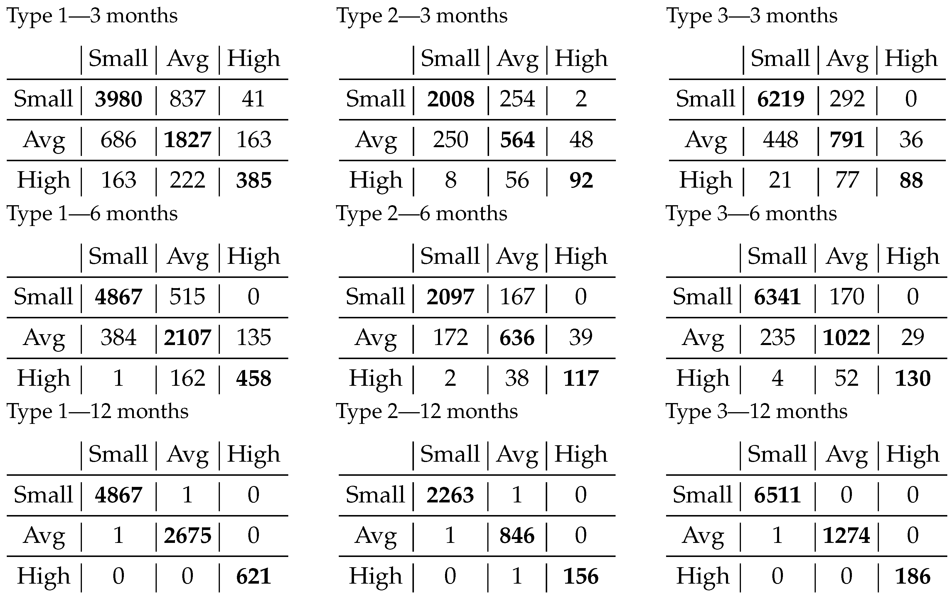
We further assess the effectiveness of the proposed method in Figure 5, which offers a detailed glimpse into the performance of our classification model. These confusion matrices encapsulate the outcomes of our classification endeavors, reflecting the model’s proficiency when confronted with a dataset spanning from 3 months to a full year of runtime. For the 12-month data, multiclass SVM was deployed, while the 3-month and 6-month data were subjected to the random forest algorithm. For each classification, the most suited identified configuration was used.

Figure 5.
Appliance classification results separated by time ranges used for computing features. The nine tables represent three types of appliances at three time intervals. One table has on the horizontal the actual class, and on the vertical the predicted one.
The progression of results in the classification, as influenced by the selected time interval, demonstrates that the number of misclassified items remains small compared to the overall sample size when we use a more extended time range. In the case of 3-month data, most of the errors in classification are with the neighbor class. When extending to 6 months of data, the overall number of wrongly classified instances is half of the initial ones, while for the further away class, it either disappears or becomes negligible.
The best results were achieved for 12 months with multiclass SVM on all types of appliances. The numbers of appliances that were misclassified was between one and three, which indicates a reliable classification. Not only has the performance improved to over 99.89%, but the very few classification errors in the confusion matrix are near the main diagonal, which means the errors are between nearby classes.
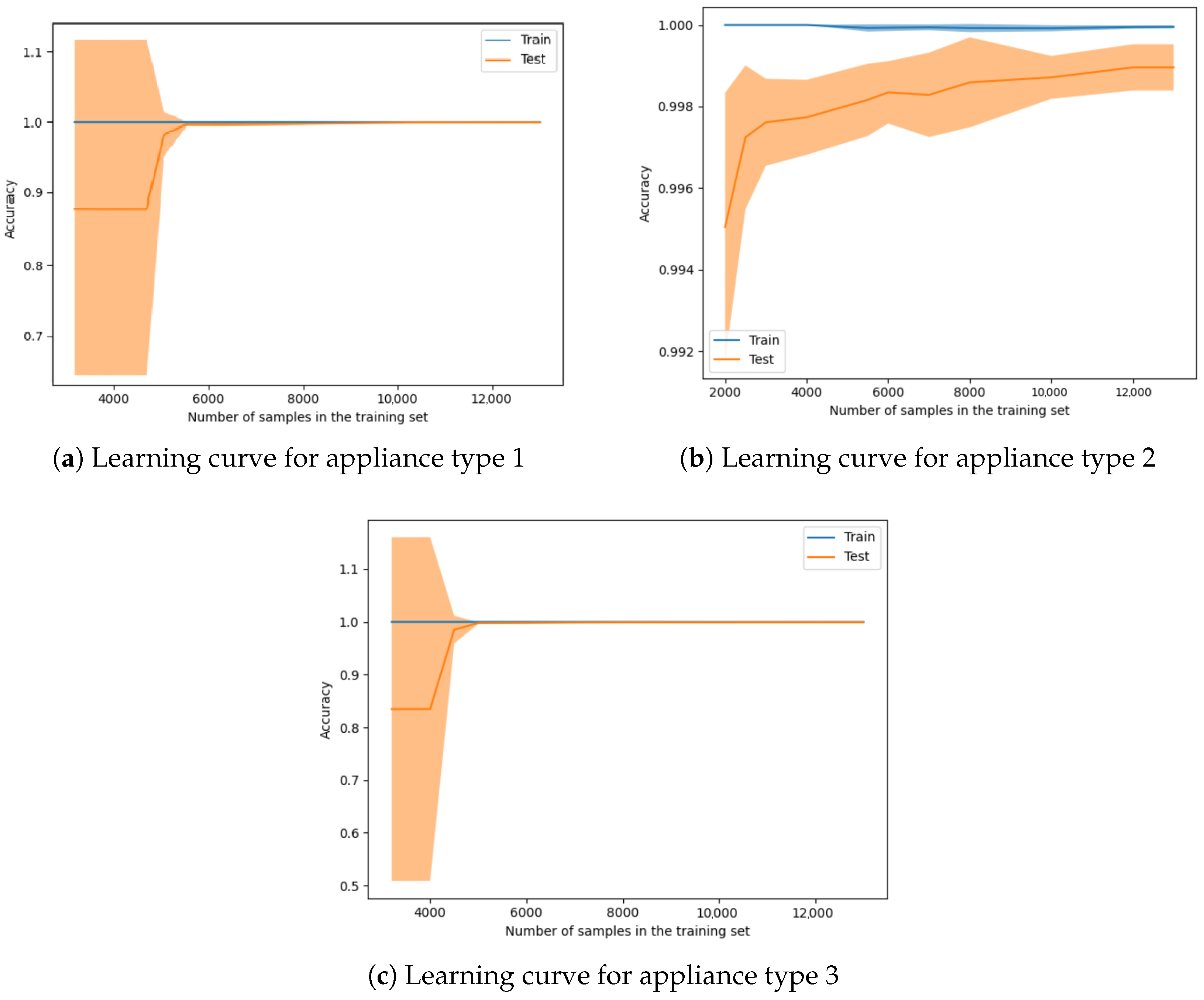
Data size dimension. We computed the learning curve for each appliance type to determine the minimal set of data needed to achieve a high-accuracy classification from the perspective of the dataset dimensions. Since the 12-month timespan leads to the best performance, the rest of the experiments were conducted with this setup. From the features perspective, we used the extended feature set, which contains both the average number of cycles and runtime per month and the information separated by weekday. Figure 6 illustrates an estimator’s training and validation scores for varying training samples. The transparent orange part from the plot represents the standard deviation. It can be observed in Figure 6a,c that until around 5000 instances, there is a high degree of deviation, which means that the model has an increased level of uncertainty.
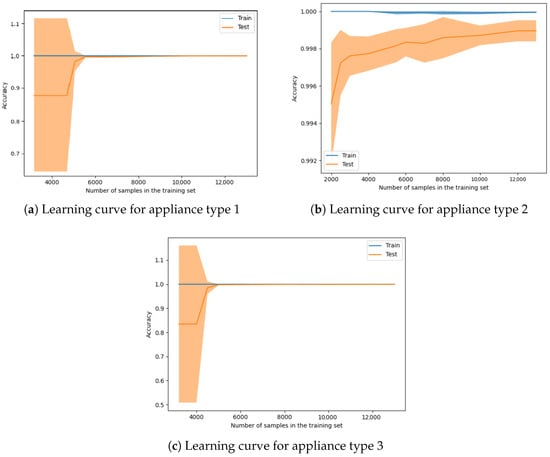
Figure 6.
Learning curve on classification using 12 months data applied on each device type.
When we used a training set of 5000 instances for all three types of devices, it resulted in an accuracy of over 99.70% with a standard deviation smaller than 0.25%. In Figure 6a,c, for appliance types 1 and 3, there is an inflection point of around 5000 instances used in the training set. In the case of appliance 2, this inflection starts earlier, but there is a smaller increase after using around 5000 devices. For all instances when using more than 10,000 samples in the training set, the increase in accuracy tends to be constant.
Feature set. We additionally assess the significance of the features employed in the classification task by employing random forest. The feature set comprises run times, cycle numbers for each weekday, and the average number of cycles and average runtime per month. Figure 7 depicts the outcomes obtained from appliance type 1 data, with blue bars indicating the feature importances within the forest and black lines representing their variability across trees. The feature importance is determined based on the mean decrease in impurity in the accumulation and the standard deviation within each tree.
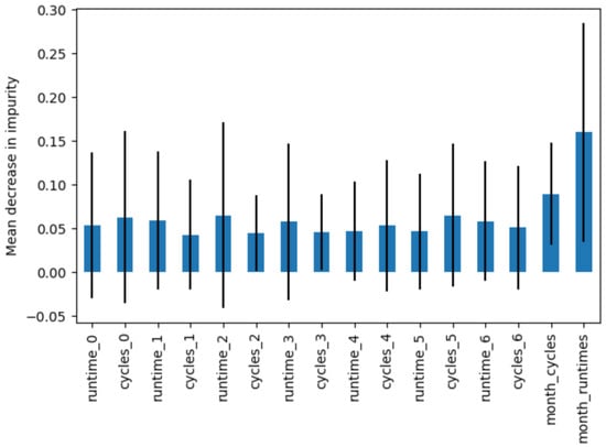
Figure 7.
Feature importance based on mean decrease in impurity for appliance type 1 data.
To investigate the impact of the feature set, we conducted a series of experiments, echoing the methodology described earlier. In this iteration, we refined our approach to focus solely on two fundamental features: the average number of monthly cycles and the average running time in seconds per month. According to Figure 7, these two features achieved the highest scores based on the mean decrease in impurity. The average number of monthly cycles and average runtime offer a condensed yet informative glimpse into the operational characteristics of the devices. By simplifying the dataset to these key metrics, we aimed to ascertain whether the day-of-the-week separation could significantly enhance the classification results. From the perspective of data size, we used the entire dataset, while for the time interval, we used all ranges from the previous set of experiments: three-month data, six-month data, and 1-year data.
The results of this refined experimentation are detailed in Table 6. This table is a comprehensive reference point, allowing us to compare the most promising outcomes for each device type across varying periods. For each device type, we showcase the best results obtained from all the classification tools from the previous set of experiments. We achieved a slightly improved classification accuracy in all experiments when using our proposed feature set.
Table 6.
Comparison results for appliance classification based on the features used for classification.
The juxtaposition of these results demonstrates the potential advantages of incorporating day-of-the-week separation into the feature engineering process. Since the results are close to one another (under 2% improvement for the extended feature set), the reduced dataset should be used if limited resources are available.
According to our experiments, in which Function 3 maintained two arguments constant and the third was used for experimentation, the best results were achieved when we used 12 months for the time interval for the recorded data, a training set of over 5k samples per device type, and an extended feature set which contained the monthly and weekday features.
5. Conclusions
This paper proposes a general method for characterizing household energy consumers based on usage patterns from raw sensor data recorded from appliances. Cluster analysis was applied in the literature reviewed to determine types of household energy consumers or types of appliances, but no similar works on determining appliance consumer class from raw sensor data that recorded device functioning information existed before. We applied our original pipeline to real household appliance data from three different types of machines recorded during one-year intervals. A cluster analysis was performed based on features to estimate the most appropriate number of clusters, and a clustering algorithm was applied to obtain labels that were further used in the classification process. From our cluster analysis, a neat separation of appliances based on their usage classes into three classes was found: low-used, medium-used, and highly used devices.
We investigated the minimal requirements for a good classification for an appliance-specific dataset from three dimensions. They are: (i) the needed time interval to record sensor data, (ii) data size—the number of instances needed for the training set, (iii) the feature set used.
From a time interval perspective, we obtained an increase in the performance of up to 15% when using data from one entire year compared to smaller intervals, and the classification achieved an accuracy of over 99.89% for all the device types, with at most three appliances misclassified, all of them in the nearby class.
Looking from the perspective of the training set’s dimensionality, using at least 5000 instances per device type led to an accuracy of over 99.80%. Using a smaller quantity of data for the training set gives a high standard deviation for appliance types 1 and 3.
From a feature set perspective, from computed time series data, we proposed a separation on different granularity levels for the amount of time. We found a significant influence of the average number of running cycles and the average runtime seconds per month for features, as well as of separating them per weekday. We compared the results of the extended set of features with the best ones we achieved when using only the average per month, and we obtained slightly better results in all our experiments.
Author Contributions
Conceptualization, R.L.P.; methodology, R.L.P. and R.P.; software, R.L.P.; validation, R.L.P.; formal analysis, R.L.P.; investigation, R.L.P.; resources, R.L.P., R.T. and R.P.; data curation, R.L.P. and R.T.; writing—original draft preparation, R.L.P.; writing—review and editing, R.L.P., R.P. and R.T.; visualization, R.L.P.; supervision, R.P. All authors have read and agreed to the published version of the manuscript.
Funding
This research received no external funding.
Institutional Review Board Statement
Not applicable.
Informed Consent Statement
Not applicable.
Data Availability Statement
The authors do not have permission to disclose the data.
Conflicts of Interest
The authors declare no conflicts of interest.
References
- Firte, C.; Iamnitchi, L.; Portase, R.; Tolas, R.; Potolea, R.; Dinsoreanu, M.; Lemnaru, C. Knowledge inference from home appliances data. In Proceedings of the 2022 IEEE 18th International Conference on Intelligent Computer Communication and Processing (ICCP), Cluj-Napoca, Romania, 22–24 September 2022; pp. 237–243. [Google Scholar] [CrossRef]
- Babaei, M.; Abazari, A.; Soleymani, M.M.; Ghafouri, M.; Muyeen, S.; Beheshti, M.T. A data-mining based optimal demand response program for smart home with energy storages and electric vehicles. J. Energy Storage 2021, 36, 102407. [Google Scholar] [CrossRef]
- EPA. U.S. Environmental Protection Agency. Electricity Customers. Available online: https://www.epa.gov/energy/electricity-customers (accessed on 17 October 2023).
- Kong, W.; Dong, Z.Y.; Jia, Y.; Hill, D.J.; Xu, Y.; Zhang, Y. Short-term residential load forecasting based on LSTM recurrent neural network. IEEE Trans. Smart Grid 2017, 10, 841–851. [Google Scholar] [CrossRef]
- Koop, S.; Van Dorssen, A.; Brouwer, S. Enhancing domestic water conservation behaviour: A review of empirical studies on influencing tactics. J. Environ. Manag. 2019, 247, 867–876. [Google Scholar] [CrossRef] [PubMed]
- Muhsen, D.H.; Haider, H.T.; Al-Nidawi, Y.; Khatib, T. Optimal home energy demand management based multi-criteria decision making methods. Electronics 2019, 8, 524. [Google Scholar] [CrossRef]
- Fulcher, B.D. Feature-based time-series analysis. In Feature Engineering for Machine Learning and Data Analytics; CRC Press: Boca Raton, FL, USA, 2018; pp. 87–116. [Google Scholar]
- Bonifati, A.; Buono, F.D.; Guerra, F.; Tiano, D. Time2Feat: Learning interpretable representations for multivariate time series clustering. Proc. VLDB Endow. 2022, 16, 193–201. [Google Scholar] [CrossRef]
- Olariu, E.M.; Tolas, R.; Portase, R.; Dinsoreanu, M.; Potolea, R. Modern approaches to preprocessing industrial data. In Proceedings of the 2020 IEEE 16th International Conference on Intelligent Computer Communication and Processing (ICCP), Cluj-Napoca, Romania, 3–5 September 2020; pp. 221–226. [Google Scholar] [CrossRef]
- Lin, J.; Williamson, S.; Borne, K.; DeBarr, D. Pattern recognition in time series. In Advances in Machine Learning and Data Mining for Astronomy; Citeseer: Princeton, NJ, USA, 2012; Volume 1, p. 3. [Google Scholar]
- Croston, J.D. Forecasting and stock control for intermittent demands. J. Oper. Res. Soc. 1972, 23, 289–303. [Google Scholar] [CrossRef]
- Wang, X.; Mueen, A.; Ding, H.; Trajcevski, G.; Scheuermann, P.; Keogh, E. Experimental comparison of representation methods and distance measures for time series data. Data Min. Knowl. Discov. 2013, 26, 275–309. [Google Scholar] [CrossRef]
- Laurinec, P.; Lucká, M. Interpretable multiple data streams clustering with clipped streams representation for the improvement of electricity consumption forecasting. Data Min. Knowl. Discov. 2019, 33, 413–445. [Google Scholar] [CrossRef]
- Fu, X.; Zeng, X.J.; Feng, P.; Cai, X. Clustering-based short-term load forecasting for residential electricity under the increasing-block pricing tariffs in China. Energy 2018, 165, 76–89. [Google Scholar] [CrossRef]
- Ramnath, G.S.; Muyeen, S.; Kotecha, K. Household Electricity Consumer Classification Using Novel Clustering Approach, Review, and Case Study. Electronics 2022, 11, 2302. [Google Scholar] [CrossRef]
- Figueiredo, V.; Rodrigues, F.; Vale, Z.; Gouveia, J.B. An electric energy consumer characterization framework based on data mining techniques. IEEE Trans. Power Syst. 2005, 20, 596–602. [Google Scholar] [CrossRef]
- Chicco, G. Overview and performance assessment of the clustering methods for electrical load pattern grouping. Energy 2012, 42, 68–80. [Google Scholar] [CrossRef]
- Ofetotse, E.L.; Essah, E.A.; Yao, R. Evaluating the determinants of household electricity consumption using cluster analysis. J. Build. Eng. 2021, 43, 102487. [Google Scholar] [CrossRef]
- Hur, C.H.; Lee, H.E.; Kim, Y.J.; Kang, S.G. Semi-supervised domain adaptation for multi-label classification on nonintrusive load monitoring. Sensors 2022, 22, 5838. [Google Scholar] [CrossRef]
- Chen, Y.C.; Ko, Y.L.; Peng, W.C.; Lee, W.C. Mining appliance usage patterns in smart home environment. In Proceedings of the Advances in Knowledge Discovery and Data Mining: 17th Pacific-Asia Conference, PAKDD 2013, Gold Coast, Australia, 14–17 April 2013; Proceedings, Part I 17. Springer: Berlin/Heidelberg, Germany, 2013; pp. 99–110. [Google Scholar]
- Likas, A.; Vlassis, N.; Verbeek, J.J. The global k-means clustering algorithm. Pattern Recognit. 2003, 36, 451–461. [Google Scholar] [CrossRef]
- Mohamad, I.B.; Usman, D. Standardization and its effects on K-means clustering algorithm. Res. J. Appl. Sci. Eng. Technol. 2013, 6, 3299–3303. [Google Scholar] [CrossRef]
- Haben, S.; Singleton, C.; Grindrod, P. Analysis and clustering of residential customers energy behavioral demand using smart meter data. IEEE Trans. Smart Grid 2015, 7, 136–144. [Google Scholar] [CrossRef]
- Yilmaz, S.; Chambers, J.; Patel, M.K. Comparison of clustering approaches for domestic electricity load profile characterisation-Implications for demand side management. Energy 2019, 180, 665–677. [Google Scholar] [CrossRef]
- Syakur, M.; Khotimah, B.; Rochman, E.; Satoto, B.D. Integration k-means clustering method and elbow method for identification of the best customer profile cluster. IOP Conf. Ser. Mater. Sci. Eng. 2018, 336, 012017. [Google Scholar] [CrossRef]
- Kodinariya, T.M.; Makwana, P.R. Review on determining number of Cluster in K-Means Clustering. Int. J. 2013, 1, 90–95. [Google Scholar]
- Caliński, T.; JA, H. A Dendrite Method for Cluster Analysis. Commun. Stat.—Theory Methods 1974, 3, 1–27. [Google Scholar] [CrossRef]
- Davies, D.L.; Bouldin, D.W. A Cluster Separation Measure. IEEE Trans. Pattern Anal. Mach. Intell. 1979, PAMI-1, 224–227. [Google Scholar] [CrossRef]
- Sousa, M.; Tomé, A.M.; Moreira, J. Long-term forecasting of hourly retail customer flow on intermittent time series with multiple seasonality. Data Sci. Manag. 2022, 5, 137–148. [Google Scholar] [CrossRef]
- Goldberger, J.; Hinton, G.E.; Roweis, S.; Salakhutdinov, R.R. Neighbourhood components analysis. Adv. Neural Inf. Process. Syst. 2004, 17, 513–520. [Google Scholar]
- Weston, J.; Watkins, C. Multi-Class Support Vector Machines; Technical Report; Citeseer: Princeton, NJ, USA, 1998. [Google Scholar]
- Breiman, L. Random forests. Mach. Learn. 2001, 45, 5–32. [Google Scholar] [CrossRef]
- Rish, I. An empirical study of the naive Bayes classifier. In Proceedings of the IJCAI 2001 Workshop on Empirical Methods in Artificial Intelligence, Seattle, WA, USA, 4–6 August 2001; Volume 3, pp. 41–46. [Google Scholar]
- Windeatt, T. Accuracy/diversity and ensemble MLP classifier design. IEEE Trans. Neural Netw. 2006, 17, 1194–1211. [Google Scholar] [CrossRef]
- Sadeghianpourhamami, N.; Ruyssinck, J.; Deschrijver, D.; Dhaene, T.; Develder, C. Comprehensive feature selection for appliance classification in NILM. Energy Build. 2017, 151, 98–106. [Google Scholar] [CrossRef]
- Liu, H.; Wu, H.; Yu, C. A hybrid model for appliance classification based on time series features. Energy Build. 2019, 196, 112–123. [Google Scholar] [CrossRef]
- D’hulst, R.; Labeeuw, W.; Beusen, B.; Claessens, S.; Deconinck, G.; Vanthournout, K. Demand response flexibility and flexibility potential of residential smart appliances: Experiences from large pilot test in Belgium. Appl. Energy 2015, 155, 79–90. [Google Scholar] [CrossRef]
- Cruz, C.; Tostado-Véliz, M.; Palomar, E.; Bravo, I. Pattern-driven behaviour for demand-side management: An analysis of appliance use. Energy Build. 2024, 308, 113988. [Google Scholar] [CrossRef]
- Zufferey, D.; Gisler, C.; Abou Khaled, O.; Hennebert, J. Machine learning approaches for electric appliance classification. In Proceedings of the 2012 11th International Conference on Information Science, Signal Processing and their Applications (ISSPA), Montreal, QC, Canada, 2–5 July 2012; pp. 740–745. [Google Scholar]
- Shafqat, W.; Lee, K.T.; Kim, D.H. A Comprehensive Predictive-Learning Framework for Optimal Scheduling and Control of Smart Home Appliances Based on User and Appliance Classification. Sensors 2022, 23, 127. [Google Scholar] [CrossRef] [PubMed]
- Portase, R.; Tolas, R.; Potolea, R. MEDIS: Analysis Methodology for Data with Multiple Complexities. In Proceedings of the Proceedings of the 13th International Joint Conference on Knowledge Discovery, Knowledge Engineering and Knowledge Management (IC3K 2021), Online, 25–27 October 2021; pp. 191–198. [Google Scholar]
- Pedregosa, F.; Varoquaux, G.; Gramfort, A.; Michel, V.; Thirion, B.; Grisel, O.; Blondel, M.; Prettenhofer, P.; Weiss, R.; Dubourg, V.; et al. Scikit-learn: Machine Learning in Python. J. Mach. Learn. Res. 2011, 12, 2825–2830. [Google Scholar]


Disclaimer/Publisher’s Note: The statements, opinions and data contained in all publications are solely those of the individual author(s) and contributor(s) and not of MDPI and/or the editor(s). MDPI and/or the editor(s) disclaim responsibility for any injury to people or property resulting from any ideas, methods, instructions or products referred to in the content. |
© 2024 by the authors. Licensee MDPI, Basel, Switzerland. This article is an open access article distributed under the terms and conditions of the Creative Commons Attribution (CC BY) license (https://creativecommons.org/licenses/by/4.0/).