Strategy of Flywheel–Battery Hybrid Energy Storage Based on Optimized Variational Mode Decomposition for Wind Power Suppression

Abstract

The fluctuation and intermittency of wind power generation seriously affect the stability and security of power grids. Aiming at smoothing wind power fluctuations, this paper proposes a flywheel–battery hybrid energy storage system (HESS) based on optimal variational mode decomposition (VMD). Firstly, the grid-connected power and charging–discharging power of the HESS are determined based on the sliding average algorithm. Secondly, the VMD algorithm, optimized using long short-term memory (LSTM), is used to decompose the hybrid energy storage power (HESP) into a series of sub-modes with frequencies from low to high. Then, the state of charge of the battery energy storage system and the speed of the flywheel energy storage system are monitored in real time, and the primary power of the HESS is modified according to the rules formulated by fuzzy control. Finally, through a simulation example, it is concluded that the method meets the requirements of smoothing wind power fluctuations and gives full play to the characteristics of energy storage battery and flywheel energy storage to ensure the stable operation of the energy storage system. The method presented in this paper can provide a reference for HESP configuration and control operation strategy formulation.

1. Introduction

In recent years, the wind power industry has developed rapidly around the world. For example, in China, wind power generation in 2023 reached 809 billion KWH, a year-on-year increase of 12.3%. The utilization rate of wind power has also increased yearly, but its random and intermittent characteristics have had a great impact on the power grid [1]. It has become urgent for the new generation of power grids to reduce the influence of the wind power grid connection by suppressing wind power fluctuation using key technology. In order to avoid adverse effects, wind power plants usually need to be equipped with corresponding energy storage devices to control wind power fluctuations within a safe range [2].

Energy storage system devices can generally be divided into two categories [3,4]: energy-type energy storage and power-type energy storage. Energy-type energy storage is mainly represented by batteries, which have the advantage of a high energy density. However, compared to power-type energy storage, their power density is smaller and their response time is longer, and they are usually used to address high-energy and low-frequency power fluctuations. Supercapacitor, superconducting magnetic, and flywheel energy storage, as representatives of power-type energy storage, have the advantages of high power density and frequent charge and discharge. However, compared to energy-type energy storage, their energy density is smaller, so they are usually used to handle power fluctuations with a low volume and high frequency [5].

Scholars have conducted many studies on wind power fluctuations. Based on the relationships among the time constant, volatility, and energy storage capacity, Refs. [6,7,8] optimized a hybrid energy storage model with a first-order low-pass filter. However, there is a certain time lag in the implementation of the model, and it is difficult to extract the eigenvalues accurately. Ref. [9] used wavelet packet decomposition to process the original power signal for wind farm power fluctuations, and then used the corresponding energy storage device to calm the power fluctuations. The wavelet packet decomposition method uses a lower high-frequency component and a higher low-frequency component after signal decomposition. Ref. [10] proposed a method that uses empirical mode decomposition (EMD) to process the original wind power data and then uses an energy storage device to smooth the wind power fluctuation, but the power fluctuation constraint is not fully considered. Refs. [11,12,13] introduced EMD to decompose the original wind power data to obtain high- and low-frequency power and combined it with Hilbert transform to obtain the instantaneous frequency of the inherent mode function (IMF), select the boundary frequency, and adjust the charge–discharge power of the energy storage system by monitoring the state of charge (SOC) of the battery energy storage system (BESS) so as to extend the service life of the battery.

Since modal components with similar frequencies cannot be accurately separated out in EMD recursive decomposition, mode aliasing occurs, which is easily affected by the sampling rate, and recursive screening cannot correct errors. Compared to EMD, variational mode decomposition (VMD) can solve problems such as the mode aliasing phenomenon in signal decomposition and characteristic frequencies that are difficult to distinguish due to noise interference [14,15]. Additionally, the VMD rate is high and has good robustness.

Long short-term memory (LSTM) overcomes the defects of recurrent neural networks (RNNs) and challenges such as gradient disappearance, gradient explosion, and lack of long-term memory in learning and training [16,17]. LSTM is widely used in the field of time series prediction, such as power load prediction [18,19,20] and wind speed prediction [21,22]. In Ref. [23], a VMD and LSTM fusion model was used to forecast the sales volume of new energy vehicles. Ref. [24] proposed a short-time traffic flow prediction method based on VMD and LSTM neural networks. Ref. [25], based on VMD-LSTM fuel price forecast, achieved the best performance. Ref. [26] proposed a variational mode decomposition–long short-term memory (VMD-LSTM) wind power forecasting method, which has good performance. With the development of deep learning, a hybrid model of LSTM and VMD has become the future trend [27].

Aiming at smoothing the power fluctuation of wind power generation, a power decomposition method of a flywheel–battery hybrid energy storage system (HESS) based on LSTM-optimized VMD is proposed. Firstly, the grid-connected power and HESS power are calculated based on the sliding average algorithm. Secondly, the decomposition algorithm based on LSTM-optimized VMD is used to decompose the hybrid energy storage power (HESP) into a series of sub-modes with frequencies from low to high to complete the initial power distribution of the HESS. Then, the state of charge of the BESS and the speed of the flywheel energy storage system (FESS) are monitored in real time, and the primary power of the HESS is modified according to the rules formulated by fuzzy control. Finally, through a simulation example, it is concluded that the HESS can meet the requirements of smooth wind power fluctuations and give full play to the characteristics of energy storage battery and flywheel energy storage to ensure the stable operation of the energy storage system.

The original contributions of this paper are as follows.

(1)

The sliding average algorithm is used to determine the charging–discharging power grid power and the HESS;

(2)

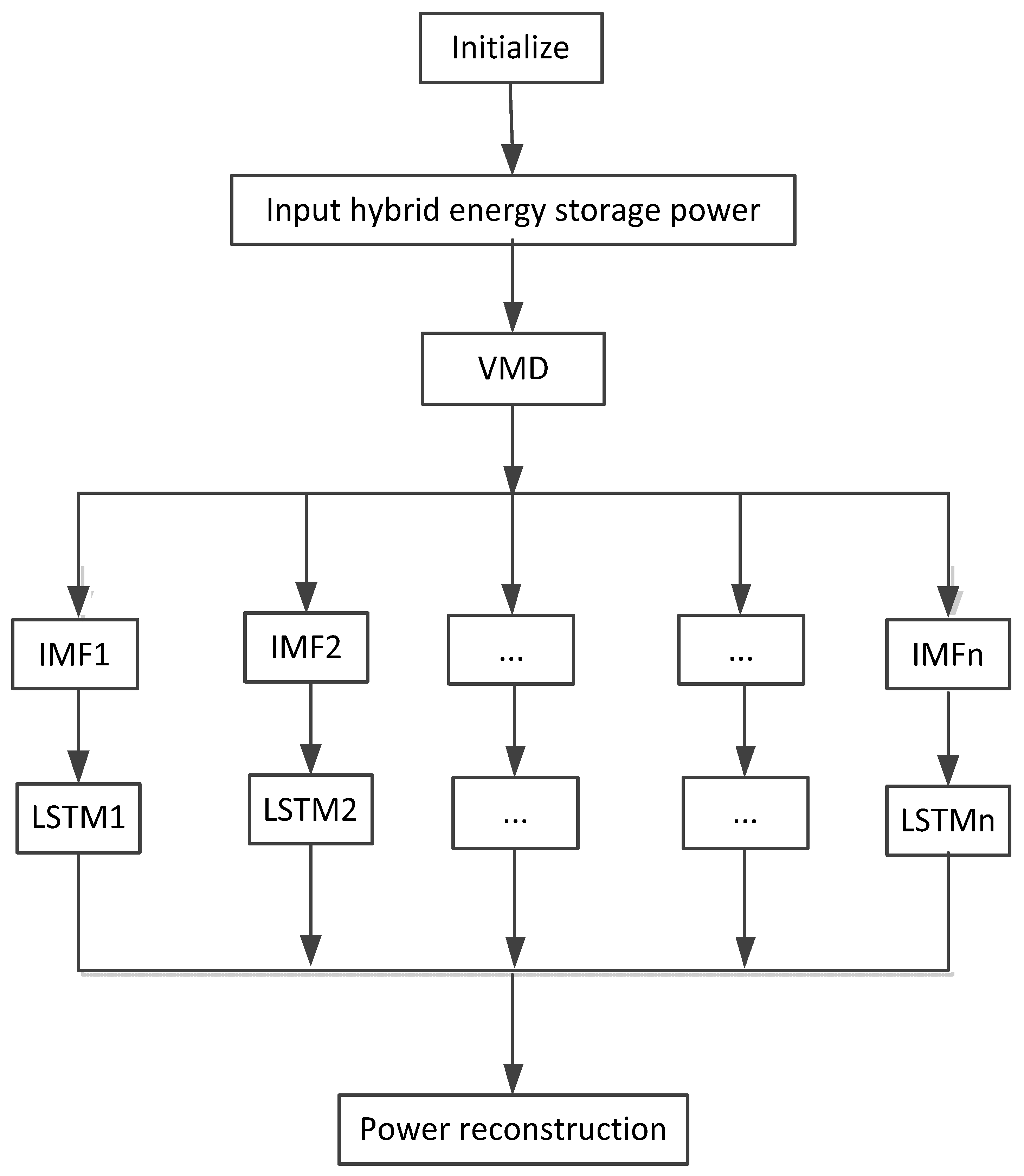
The variational mode decomposition algorithm optimized with LSTM is used to decompose the HESP into a series of sub-modes with frequencies from low to high to complete the primary power distribution of the HESS;

(3)

The state of charge of the BESS and the speed of the FESS are monitored in real time, and the primary power of the HESS is modified according to the rules formulated by fuzzy control;

(4)

The feasibility and superiority of the proposed method are verified by comparative analysis of the curves with LSTM optimization and without LSTM optimization.

The structure of the paper is organized as follows. In Section 2, the principle of the LSTM-optimized VMD algorithm is introduced in detail. In Section 3, first, the sliding average algorithm is used to determine the charging–discharging power grid power and the HESS. Second, the LSTM-optimized variational mode decomposition algorithm is used to decompose the HESP into a series of sub-modes with frequencies from low to high to complete the primary power distribution of the HESS, and the primary power of the HESS is modified according to the rules formulated by fuzzy control. In Section 4, the feasibility and superiority of the proposed method are verified using a simulation example.

2. Variational Mode Decomposition of Power in HESS

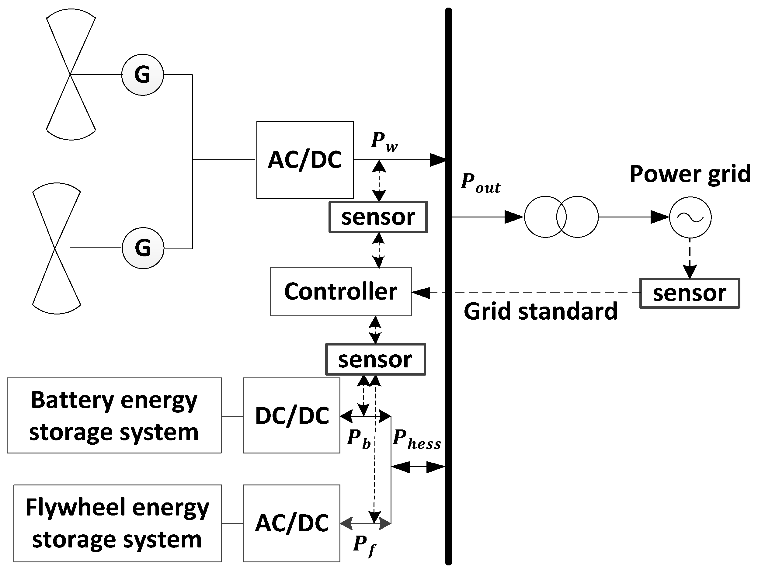
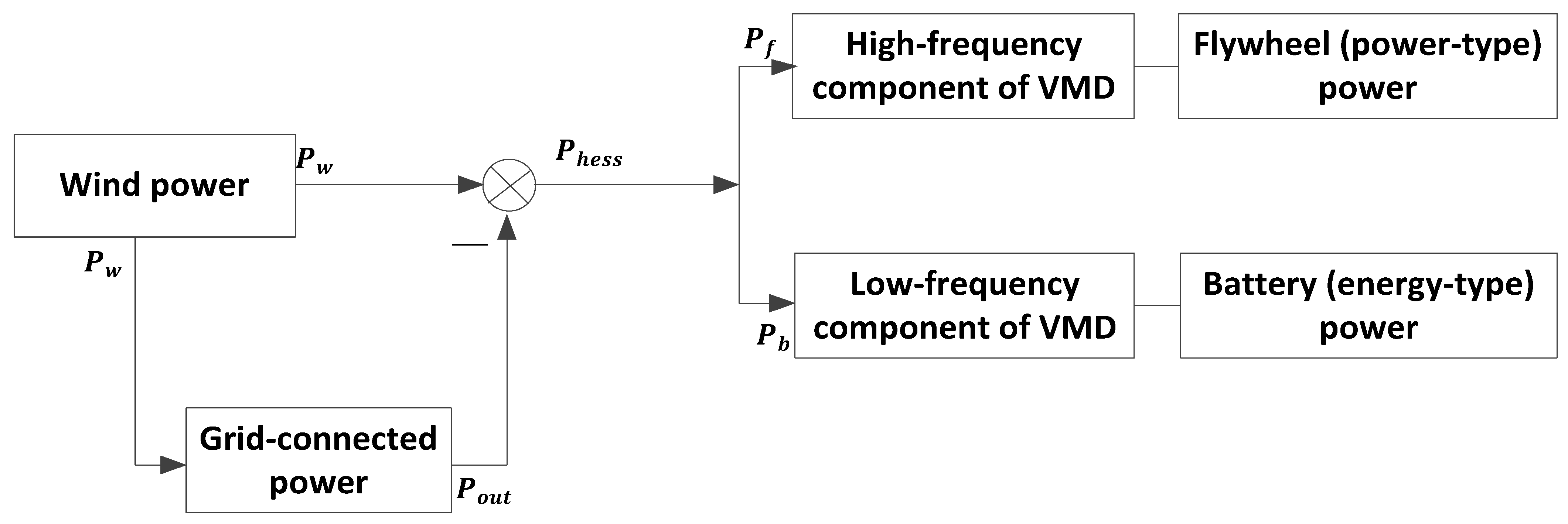
2.1. Flywheel–Battery HESS

With the development of smart grids, the demand for energy storage technology will become more diverse. It is difficult for any single energy storage technology to fully take into account the dual requirements of the power density and energy density of power grid frequency modulation and peak regulation, which easily cause declines in energy efficiency and durability, restricting the development of the energy storage industry. Therefore, the use of hybrid energy storage forms and the combination of energy storage systems with different performance levels can give full play to the advantages of different energy storage technologies. The development and application trend of energy storage technology is to meet the needs of power and energy and other aspects.

A diagram of a wind power flywheel–battery HESS and its grid-connected structure is shown in Figure 1. The structure is mainly composed of three parts: a wind farm, a BESS (energy-type), and a FESS (power-type) (composed of HESS and control system). The function of the control system is to collect the real-time power signal of the wind farm and control the charging–discharging state of the HESS in real time under the constraints of the grid-connected wind power grid standard to effectively suppress the fluctuation of wind power output.

According to Figure 1, the power relationship of the HESS is as follows:

$$P_w=P_{out}+P_{hess}=P_{out}+P_b+P_f$$

(1)

where $P_w$ is the active power in MW emitted by the wind farm; $P_{out}$ is the grid-connected power; $P_b$ is the charge–discharge power of the BESS in the HESS; $P_f$ is the charge–discharge power of the FESS in the HESS; $P_{hess}$ is the charge–discharge power of the HESS. It is specified here that when $P_{hess}$ is positive, it means that the HESS is charged, and when $P_{hess}$ is negative, it means that the HESS is discharged.

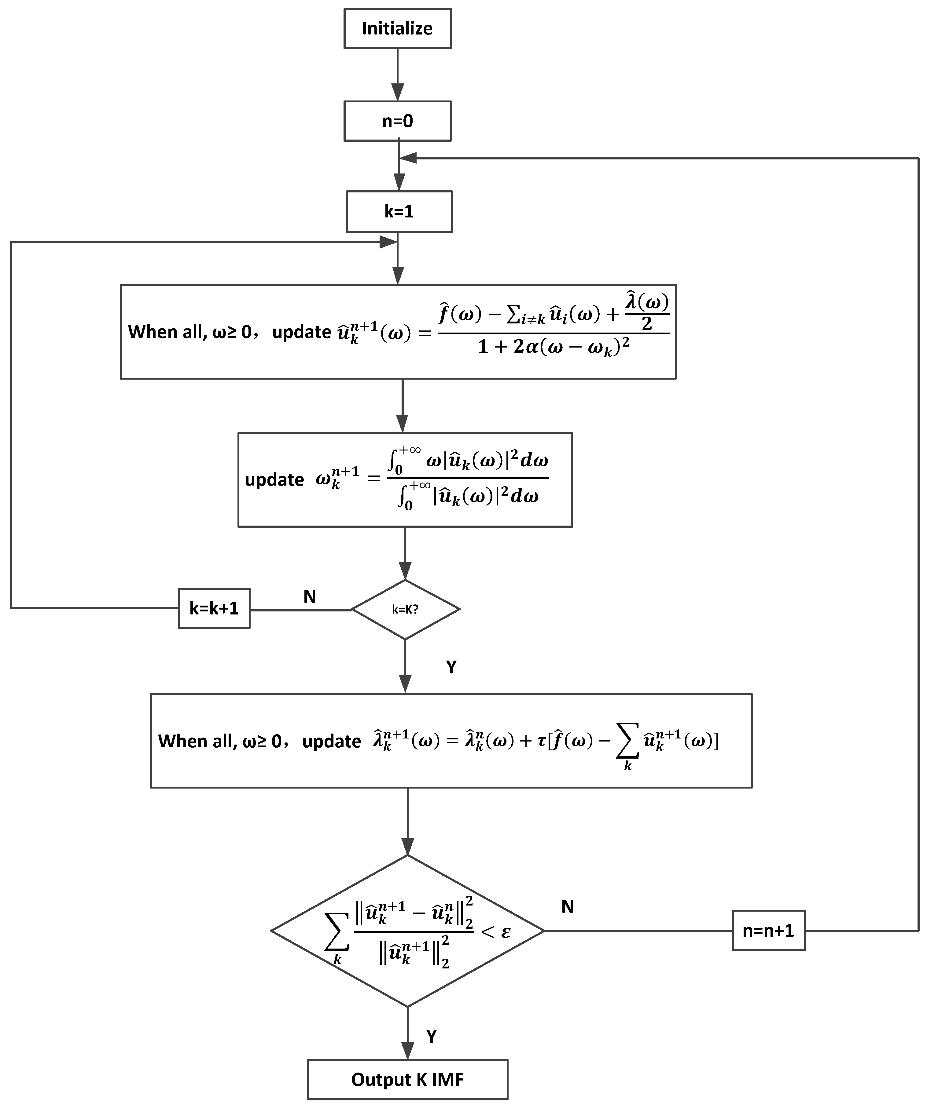
2.2. Variational Mode Decomposition

VMD is a method for the non-recursive variational mode decomposition of non-stationary signals. A new signal pre-processing method proposed by Konstantin Dragominetskiy in 2014, in which all modes are extracted simultaneously, can be used to combine signals composed of multiple frequencies. The alternating multiplier method is used to optimize multiple finite-bandwidth IMFs. The essential aim of the algorithm decomposition is to filter and reduce noise, and most of these modal components have their corresponding center frequencies.

In VMD decomposition, the input signal $f$ is decomposed into $k$ mode functions $u_k\left(t\right)$, and each $u_k\left(t\right)$ has a bandwidth with limited center frequency. The sum of the bandwidth estimates of each $u_k\left(t\right)$ is the minimum, and the constraint condition f is equal to the sum of all modes. The constraint variational equation is expressed as follows:

$$\{\begin{array}{c}\underset{\{u_k\},\{{\omega }_k\}}{\min }\left\{{\displaystyle {\displaystyle \sum }_{k=1}^K}{\Vert {𝜕}_t\left[\right(\delta (t)+\frac{j}{\pi t})\ast u_k(t)]e^{-j{w}_{k}t}\Vert }_2^2\right\}\\ s.t. {\displaystyle {\displaystyle \sum }_{k=1}^K}{u}_k=f\end{array}$$

(2)

where $\left\{u_k\right\}=\left\{u_1, u_2,\dots ,u_k\right\}$ is the set of all sub-modes; $\left\{{\omega }_k\right\}=\left\{{\omega }_1, {\omega }_2,\dots ,{\omega }_k\right\}$ is the center frequency; $\delta \left(t\right)$ is the impulse function; $k$ is the number of modes. The last determines how many modes are included in the decomposition result. If the value of K is too small, multiple real modes may be mixed together. If the value of K is too large, it may lead to the appearance of false modes.

To solve the variational constraint model, the alternating direction method of multipliers (ADMM) is used, the Lagrange operator $\lambda$ and the quadratic penalty term $\alpha$ are introduced, and the variational constraint model of the formula is transformed into an unconstrained variational expression. The augmented Lagrange expression is obtained as follows:

$$(\{u_k\},\{{\omega }_k\},\lambda )=\alpha {\displaystyle \sum }_k{\Vert {𝜕}_t\left[\left(\delta (t)+\frac{j}{\pi t}\right)\ast u_k(t)\right]e^{-j{w}_{k}t}\Vert }_2^2+{\Vert f(t)-{\displaystyle \sum }_k{u}_k(t)\Vert }_2^2+\left[\lambda \left(t\right),f\left(t\right)-{\displaystyle \sum }_k{u}_k\left(t\right)\right]$$

(3)

where $\alpha$ is the penalty factor; $\lambda$ is the Lagrange multiplication operator.

The modal components and center frequencies are optimized, the saddle points of the augmented Lagrange function are searched, and the expressions of $u_k$, ${\omega }_k$, and $\lambda$ after iteration are alternately optimized using Parseval–Fourier isothermal transform. Through calculation, the expression $u_k^{n+1}$ can be obtained as

$$u_k^{n+1}=\underset{u_k\in X}{\mathrm{argmin}}\left\{\alpha {\Vert {𝜕}_t\left[\left(\delta \left(t\right)+\frac{j}{\pi t}\right)\ast u_k\left(t\right)\right]e^{-j{w}_{k}t}\Vert }_2^2+{\Vert f\left(t\right)-{\displaystyle \sum }_k{u}_k\left(t\right)+\frac{\lambda \left(t\right)}{2}\Vert }_2^2\right\}$$

(4)

where $X$ represents the set of all $u_k$, and $n$ is the number of iterations. The Fourier isometric transform converts Equation (4) into the following frequency domain:

$${\widehat{u}}_k^{n+1}=\underset{{\widehat{u}}_k, u_k\in X}{\mathrm{argmin}}\left\{\alpha {\Vert j\left(\omega -{\omega }_k\right)\left[1+\frac{\omega }{\left|\omega \right|}\right]{\widehat{u}}_k\left(\omega \right)\Vert }_2^2+{\Vert \widehat{f}\left(\omega \right)-{\displaystyle \sum }_i{\widehat{u}}_i\left(\omega \right)+\frac{\widehat{\lambda }\left(\omega \right)}{2}\Vert }_2^2\right\}$$

(5)

where $\widehat{f}\left(\omega \right)$ is the Fourier transform of $f\left(t\right)$, and $\omega$ is the random frequency.

In the reconstructed approximation term, the conjugate symmetry of the real signal is used to change Equation (5) into a frequency non-negative half-space integral form, which is solved in the frequency domain by Parseval’s theorem.

$${\widehat{u}}_k^{n+1}=\underset{{\widehat{u}}_k, u_k\in X}{\mathrm{argmin}}\left\{{{\displaystyle \int }}_0^{\infty }\left[4\alpha {\left(\omega -{\omega }_k\right)}^2{\left|{\widehat{u}}_k\left(\omega \right)\right|}^2\right]+{\left|\widehat{f}\left(\omega \right)-{\displaystyle \sum }_i{\widehat{u}}_i\left(\omega \right)+\frac{\widehat{\lambda }\left(\omega \right)}{2}\right|}^{2}d\omega \right\}$$

(6)

For the frequency, if $\widehat{u}\left(\omega \right)=0$, then

$${\widehat{u}}_k^{n+1}\left(\omega \right)=\frac{\widehat{f}\left(\omega \right)-{\sum }_{i\ne k}{\widehat{u}}_i\left(\omega \right)+\frac{\widehat{\lambda }\left(\omega \right)}{2}}{1+2\alpha {\left(\omega -{\omega }_k\right)}^2}$$

(7)

As can be seen in Equation (7), ${\widehat{u}}_k^{n+1}\left(\omega \right)$ can be equivalent to a Wiener filter for the current residual signal. The whole spectrum of the real mode is obtained by the conjugate symmetry. Using $\left\{{\widehat{u}}_k^{n+1}\left(\omega \right)\right\},$ the inverse Fourier transform is used to obtain the time domain $\left\{u_k\left(t\right)\right\}$. Similarly, in order to obtain ${\omega }_k^{n+1}$, the smallest value of the center frequency update problem can be transformed into the corresponding frequency domain, expressed as

$${\omega }_k^{n+1}=\underset{{\omega }_k}{\mathrm{argmin}}\left\{{\displaystyle \sum }_k{\Vert {𝜕}_t\left[\left(\delta \left(t\right)+\frac{j}{\pi t}\right)\ast u_k\left(t\right)\right] e^{-j{w}_{k}t}\Vert }_2^2\right\}=\underset{{\omega }_k}{\mathrm{argmin}}\left\{{{\displaystyle \int }}_0^{\infty }\left(\omega -{\omega }_k\right){\left|{\widehat{u}}_k\left(\omega \right)\right|}^{2}d\omega \right\}$$

(8)

The center frequency is iteratively updated to

$${\omega }_k^{n+1}=\frac{{\int }_0^{+\infty }\omega {\left|{\widehat{u}}_k\left(\omega \right)\right|}^{2}d\omega }{{\int }_0^{+\infty }{\left|{\widehat{u}}_k\left(\omega \right)\right|}^{2}d\omega }$$

(9)

The Lagrange operator $\lambda \mathrm{is} \mathrm{updated} \mathrm{to}$

$${\widehat{\lambda }}_k^{n+1}\left(\omega \right)={\widehat{\lambda }}_k^n\left(\omega \right)+\tau [\widehat{f}\left(\omega \right)-{\displaystyle \sum }_k{\widehat{u}}_k^{n+1}\left(\omega \right)]$$

(10)

The precision convergence criterion $\epsilon >0$. When the accuracy meets the following requirements, the iteration process stops:

$${\displaystyle \sum }_k\frac{{\Vert {\widehat{u}}_k^{n+1}-{\widehat{u}}_k^n\Vert }_2^2}{{\Vert {\widehat{u}}_k^{n+1}\Vert }_2^2}<\epsilon$$

(11)

where ${\widehat{u}}_k^{n+1}\left(\omega \right)$, ${\widehat{\lambda }}_k^{n+1}\left(\omega \right)$, $\widehat{f}\left(\omega \right)$, and ${\widehat{u}}_i\left(\omega \right)$ are the Fourier transforms of ${\widehat{u}}_k^{n+1}\left(t\right)$, ${\widehat{\lambda }}_k^{n+1}\left(t\right), \widehat{f}\left(t\right)$, and ${\widehat{u}}_i\left(t\right)$, respectively. A flow chart of the VMD algorithm is shown in Figure 2.

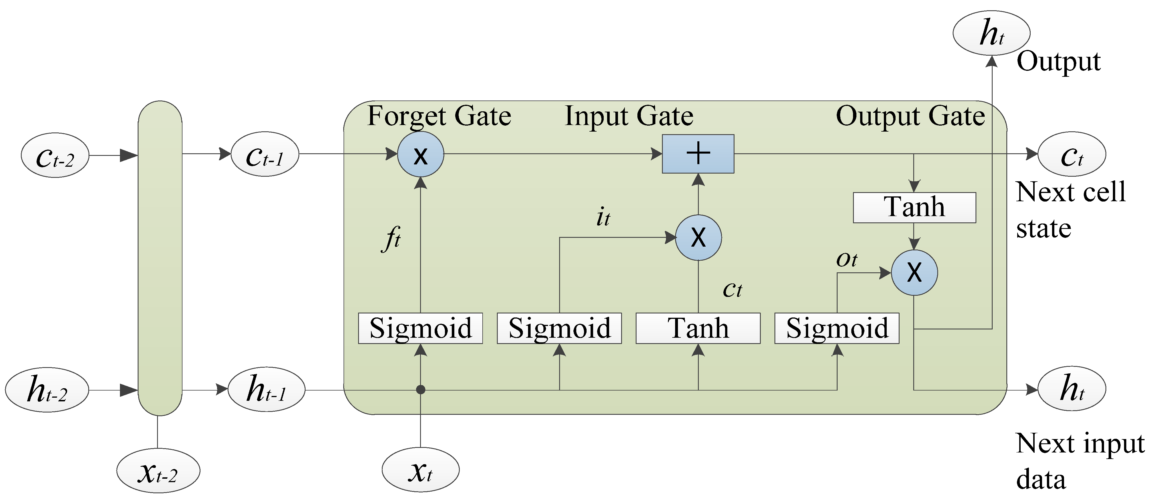
2.3. VMD Optimized with LSTM

As an excellent RNN algorithm, LSTM is widely used in the field of prediction. The structure of LSTM includes a forget gate, an input gate, and an output gate [28]. The structure of the LSTM is shown in Figure 3.

Input gate $i_t$, which controls how much of the input at the current time can enter the memory cell, is calculated as follows:

$$i_t=\sigma \left(b_i+{\omega }_{i,h}{h}_{t-1}+{\omega }_{i,x}{X}_t\right)$$

(12)

Forget gate $f_t$ determines how much of the memory cell from the previous moment will be transmitted to the current moment t.

$$f_t=\sigma \left(b_f+{\omega }_{f,h}{h}_{t-1}+{\omega }_{f,x}{x}_t\right)$$

(13)

The status of memory cell $c_t$ remembers the value of the circular layer neurons status at time t.

$$c_t=c_{t-1}\ast f_t+i_t\ast {\tilde{c}}_t$$

(14)

$${\tilde{c}}_t=tan h\left({\omega }_{c,x}{x}_t+{\omega }_{c,h}{h}_{t-1}+b_c\right)$$

Output gate $o_t$ determines what proportion of the memory value of the storage memory cell can be output.

$$o_t=\sigma \left(b_o+{\omega }_{o,h}{h}_{t-1}+{\omega }_{o,x}{x}_t\right)$$

(15)

$$h_t=o_t\ast \tan \mathrm{h}\left(c_t\right)$$

(16)

where $x_t$ is the input data at t time step, $h_t$ denotes the output data at t − 1 time step. $\sigma$ is the sigmoid function and ∗ represents the element-wise product. $\omega$ and $b$ are the weight matrices and bias vectors.

The predicted values $y_t$ can be obtained from (17) as follows:

$$y_t=f\left(b_y+{\omega }_y{h}_t\right)$$

(17)

where ${\omega }_y$ and $b_y$ are the weight matrix and bias, respectively, which determine the contribution of the extracted features. $f$ is the activation function, such as sigmoid, tanh.

In this paper, the LSTM-optimized VMD parameters are the modal number $\alpha$ and penalty factor $\alpha$. The parameters of the LSTM model are as follows: 2 input and 2 output layer variables; 100 hidden layer units; 1 hidden layer; 200 epochs; an adjustable parameter; a batch size of 128. A flow chart of the LSTM-optimized VMD algorithm [29] is shown in Figure 4.

3. HESP Distribution Strategy

3.1. Sliding Average Algorithm

The principle of the sliding average is as follows: take a sliding window of length $L$, which slides forward and backward along the sampling point. Each time the sliding window advances by one sampling point, a new sampling point is added. Similarly, every time the window goes back one sampling point, a new sampling point is added in front of it. Keep the $L$ sample points of the sliding window unchanged. This can be described by the following formula.

$$y\left(n\right)=\frac{1}{L}{\displaystyle \sum }_{i=0}^{L-1}x\left(n-i\right)$$

(18)

where x(n) and $y\left(n\right)$ are the input and filtered output values of the $NTH$ data series, and $n$ represents the sequence number of the data.

The adaptive sliding average method is used to extract grid-connected power from the original wind power data. The power of the HESS is calculated from the wind power minus the grid-connected power, and further power distribution is carried out. In this way, the phenomenon of insufficiency or over-leveling can be avoided [30]. The specific implementation method is shown in Figure 5.

3.2. First Power Allocation

After the grid-connected power and HESS power are obtained, the proposed LSTM is used to optimize the VMD parameters, and the HESS power is decomposed into a series of IMFs with frequencies from low to high. The boundary point of the high- and low-frequency components was determined by observing the signal characteristics of each IMF in the frequency domain, and the IMF is reconstructed. The reconstruction power is as follows:

$$\left\{\begin{array}{c}{P}_b\left(t\right)=P_{low}\left(t\right)={\displaystyle {\displaystyle \sum }_{k=1}^j}{u}_k\left(t\right)\\ P_f\left(t\right)=P_{high}\left(t\right)={\displaystyle {\displaystyle \sum }_{k=j+1}^k}{u}_k\left(t\right)\end{array}\right.$$

(19)

$P_{low}\left(t\right)$ is the low-frequency reconstruction of power, compensated for by the BESS, giving full play to the characteristics that lithium-ion batteries can discharge for a long time and which have a larger capacity of energy storage, meaning the HESS has a longer peak load capacity [31]. $P_{high}\left(t\right)$ is a high-frequency reconstruction power, compensated for by the FESS, giving full play to the advantages of fast charge–discharge response, high power charge and discharge, and long life, meaning the HESS has a strong frequency modulation ability, avoiding the shortcomings of the frequent changes in the charge–discharge frequency modulation of lithium-ion batteries; $j$ is the dividing point between high and low frequency.

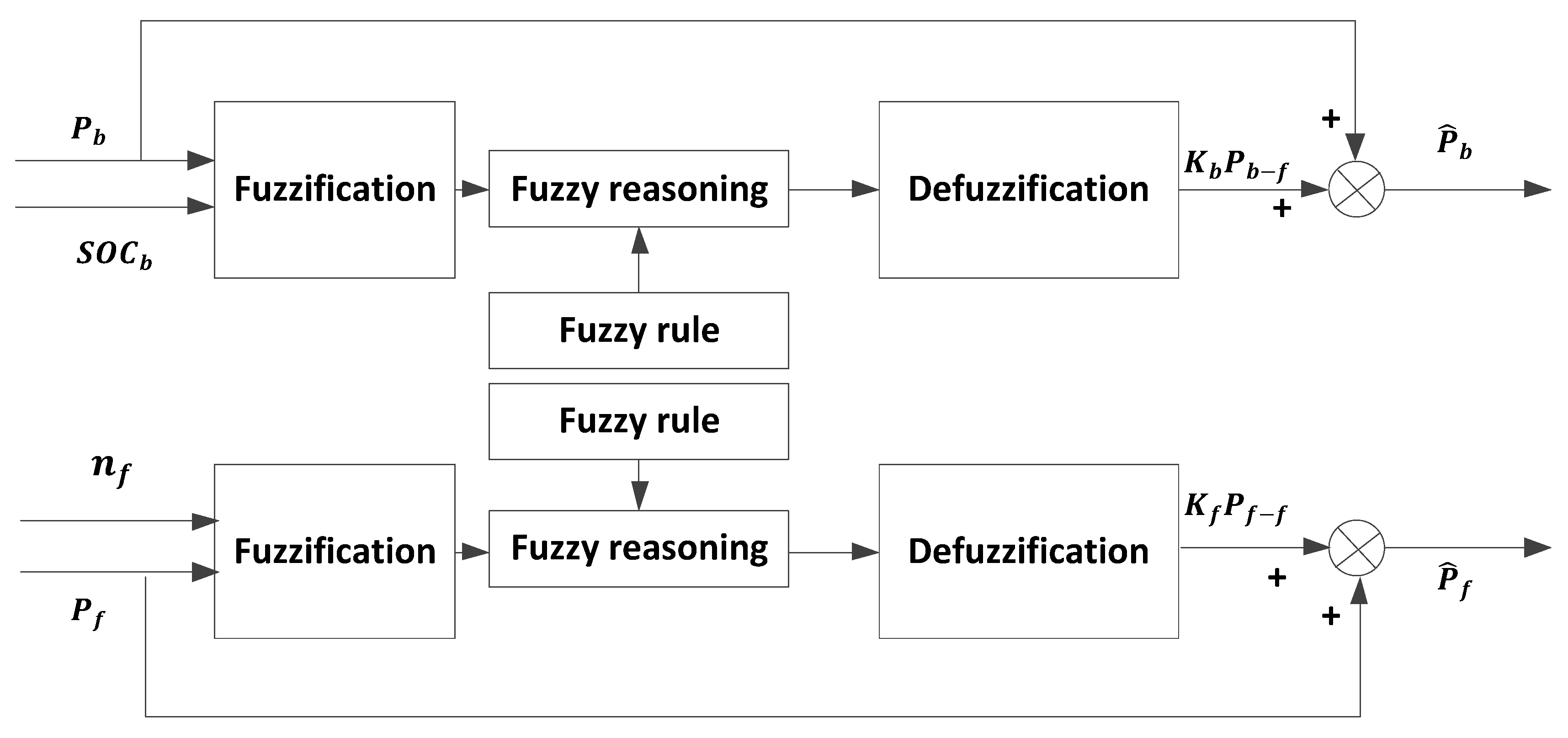
3.3. Secondary Power Correction

The VMD algorithm, after parameter optimization, completed the primary power distribution but did not take into account the fact that the overcharge and over discharge of the energy storage device will seriously affect its life, especially for the battery system, where the high cost per unit capacity limits its energy storage capacity. Therefore, based on the primary allocation, the SOC of the BESS and the speed of the FESS were considered, and the fuzzy control rules were adopted to make the second correction of the power instruction in real time [32]. The fuzzy control process is shown in Figure 6. The corrected power instruction is as follows:

$$\left\{\begin{array}{c}{\widehat{P}}_b\left(t\right)=P_b\left(t\right)+K_b\left(t\right)·P_{b-f}\left(t\right)\\ {\widehat{P}}_f\left(t\right)=P_f\left(t\right)+K_f\left(t\right)·P_{f-f}\left(t\right)\end{array}\right.$$

(20)

As shown in Figure 6, the fuzzy controller of the BESS has two input variables and one output variable.

First input variable: real-time SOC;

Theory domain range of SOC: [0, 1];

Fuzzy subset of SOC: {BVL, BS, BM, BH, BVH};

SOC level: {very low, low, moderate, high, very high};

Second input variable: normalized power instruction $P_b$;

Theory domain range of $P_b$: [−1, 1];

Fuzzy subset of $P_b$: {BNH, BNL, BZO, BPL, BPH};

Power level of $P_b$: {negative high, negative low, zero, positive low, positive high};

First output variable: correction coefficient of the power $K_b$;

Theory domain range of $K_b$: [−0.2, 0.2];

Fuzzy subset of $K_b$: {BNH, BNL, BZO, BPL, BPH};

Level of correction coefficient $K_b$: {negative high, negative low, zero, positive low, positive high}.

The fuzzy control rules of the BESS are shown in

Table 1. Fuzzy control rules of BESS.

Kb(t)		SOCb(t)
		BVL	BL	BM	BH	BVH
Pb(t)	BNH	BPH	BPL	BZO	BZO	BZO
	BNL	BPL	BPL	BZO	BZO	BNL
	BZO	BPL	BPL	BZO	BZO	BNL
	BPL	BPL	BZO	BZO	BNL	BNL
	BPH	BZO	BZO	BZO	BNL	BNH

.

As shown in Figure 6, the fuzzy controller of the FESS has two input variables and two output variables.

First input variable: flywheel speed, $n_f\left(t\right)$;

Theory domain range of $n_f\left(t\right)$: [4000, 6000];

Fuzzy subset of $n_f\left(t\right)$: {FVL, FS, FM, FH, FVH};

Flywheel speed of $n_f\left(t\right)$: {very low, low, moderate, high, very high};

Second input variable: the normalized power instruction $P_f$;

Theory domain range of $P_f$: [−1, 1];

Fuzzy subset of $P_f$: {FNH, FNL, FZO, FPL, FPH};

Power level of $P_f$: {negative high, negative low, zero, positive low, positive high};

The first output variable: correction coefficient for the power $K_f$;

Theory domain range of $K_f$: [−0.2, 0.2];

Fuzzy subset of $K_f$: {FNH, FNL, FZO, FPL, FPH};

Level of correction coefficient $K_f$: {negative high, negative low, zero, positive low, positive high}.

The fuzzy control rules of the flywheel system are shown in

Table 2. Fuzzy control rules of FESS.

Kf(t)		nf(t)
		FVL	FL	FM	FH	FVH
Pf(t)	FNH	FPH	FPL	FZO	FZO	FZO
	FNL	FPL	FPL	FZO	FZO	FNL
	FZO	FPL	FPL	FZO	FZO	FNL
	FPL	FPL	FZO	FZO	FNL	FNL
	FPH	FZO	FZO	FZO	FNL	FNH

.

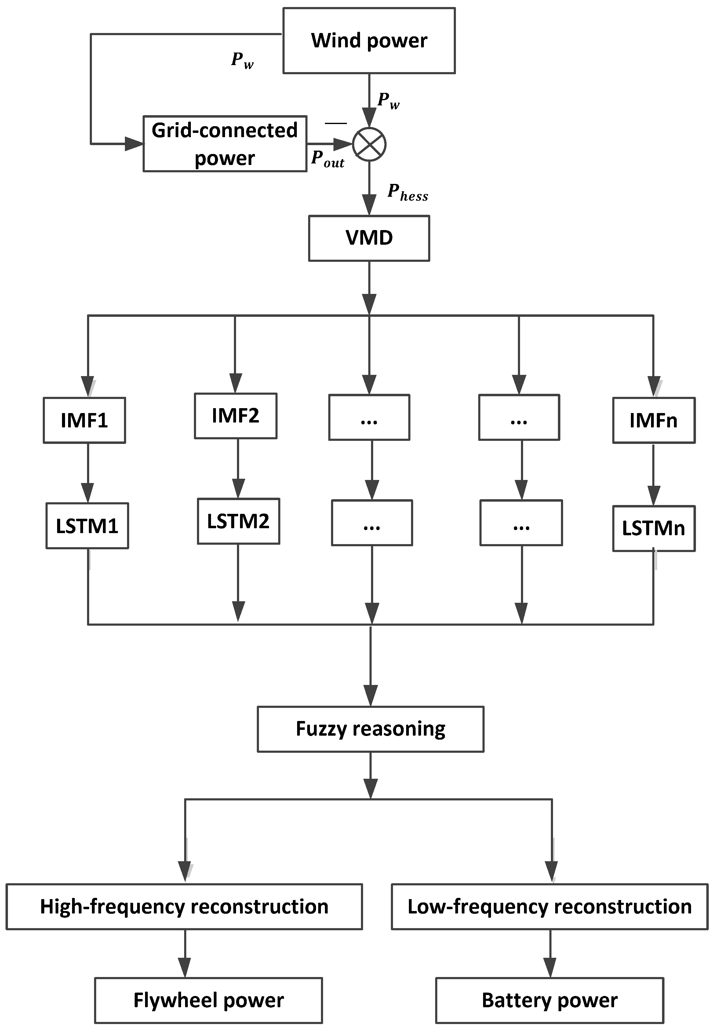
3.4. Power Distribution Flow Chart of HESS

A flow chart of the power distribution of the HESS is shown in Figure 7.

4. Simulation and Discussion

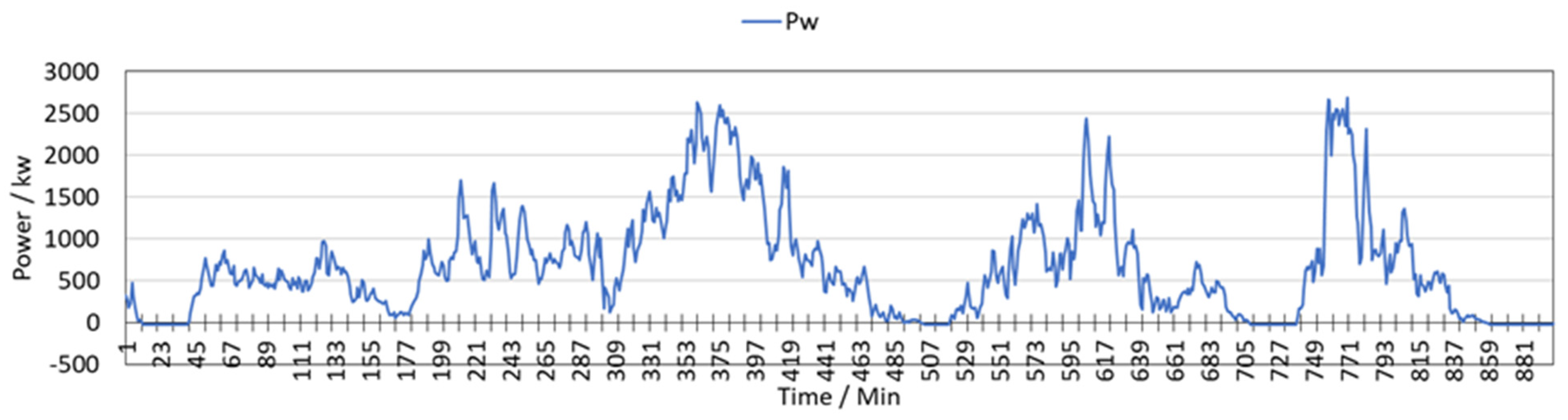
4.1. Wind Power

In order to verify the effectiveness of the proposed strategy, for this study, we used the 3.3 MW wind power data of a wind farm. The recording interval is 1 min and the sampling time is 900 min. The simulation experiment was carried out in MATLAB(R2020a), and the power curve is shown in Figure 8.

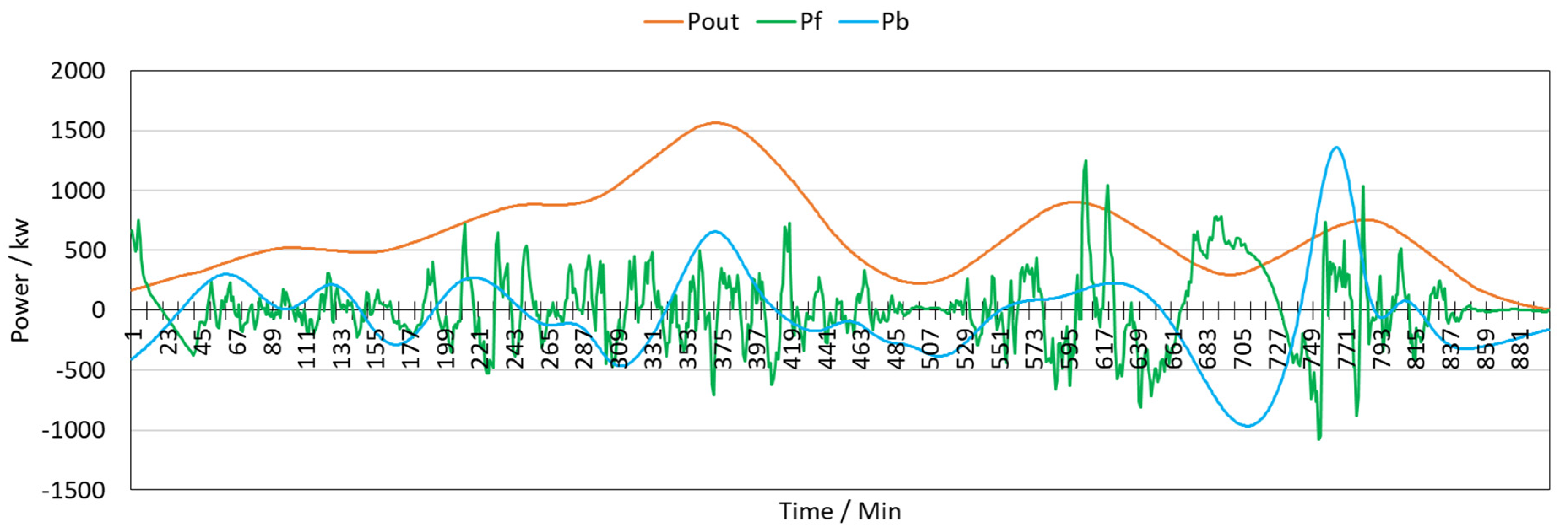
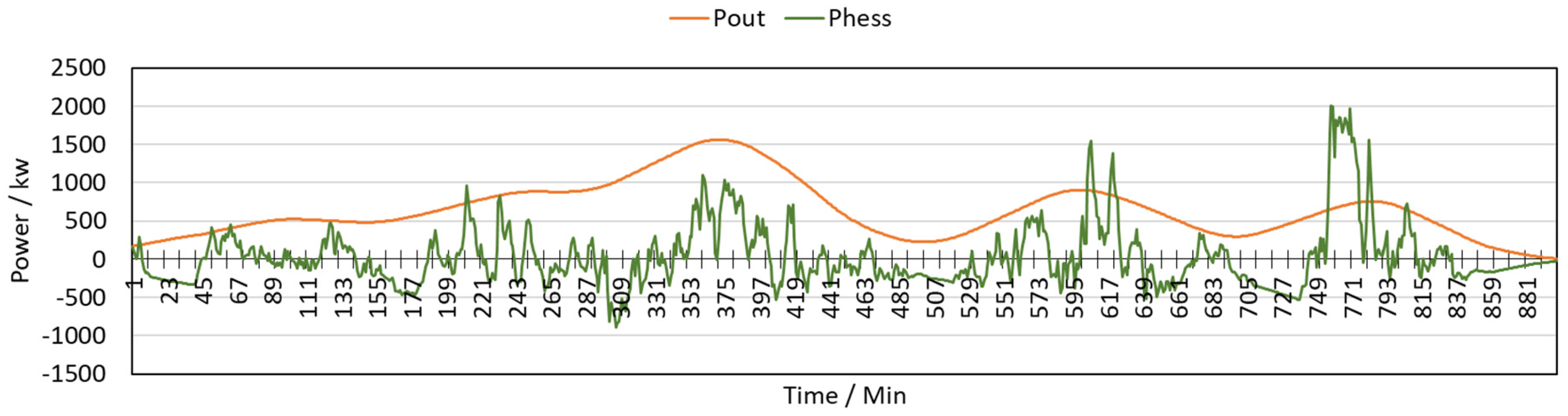
4.2. Grid-Connected Power and HESP

Using Formula (1) in Section 2.1 of this paper, the grid-connected power was extracted from the wind power data using the sliding average method. The power of the HESS was calculated by subtracting the grid-connected power from the wind power, and further power distribution was performed, as shown in Figure 9. The orange solid line is the grid-connected power, and the green solid line is the HESS power. $P_{out}$ is the grid-connected power and $P_{hess}$ is the HESS power.

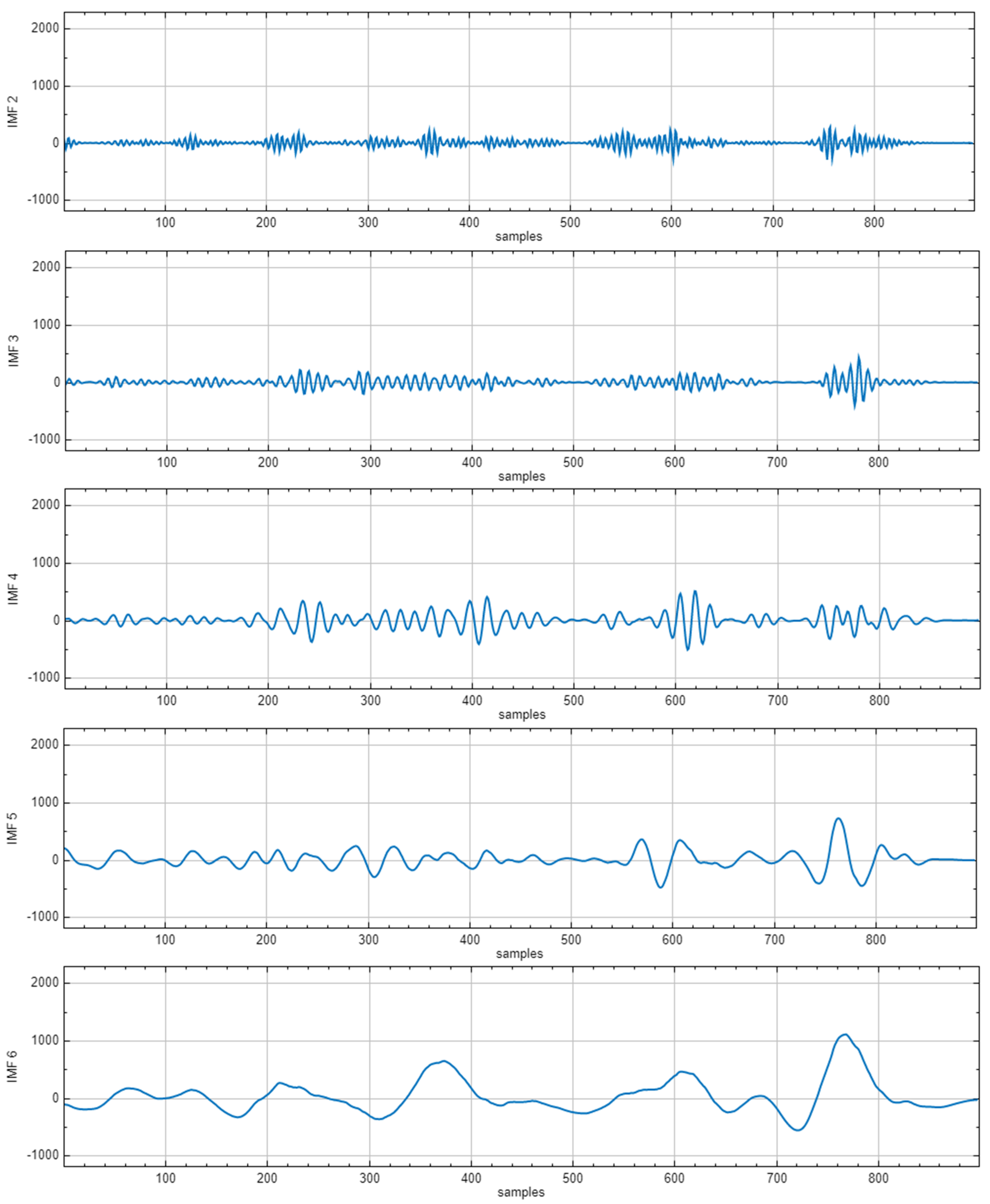
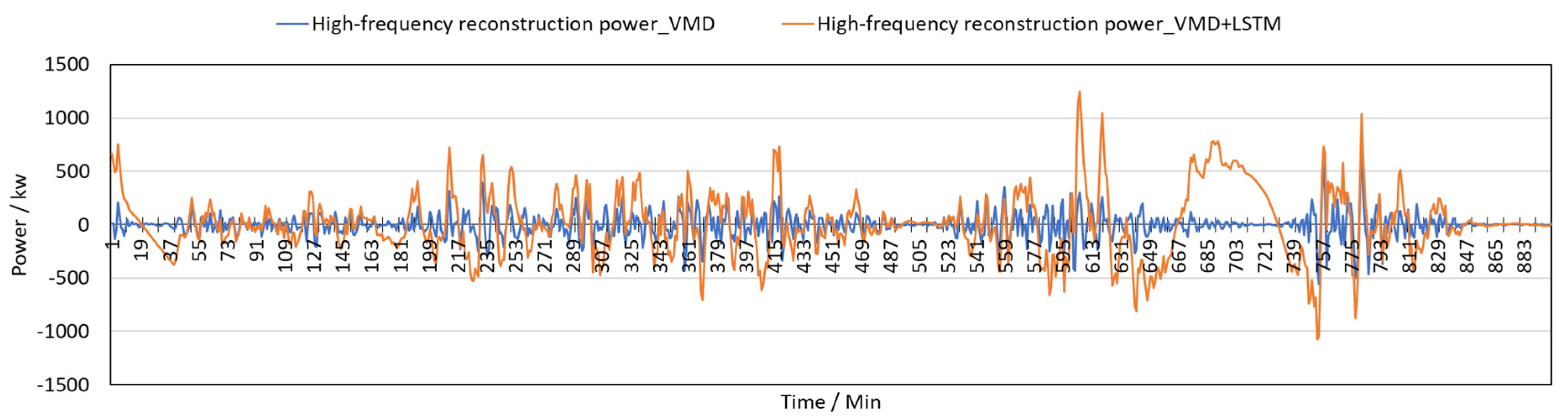
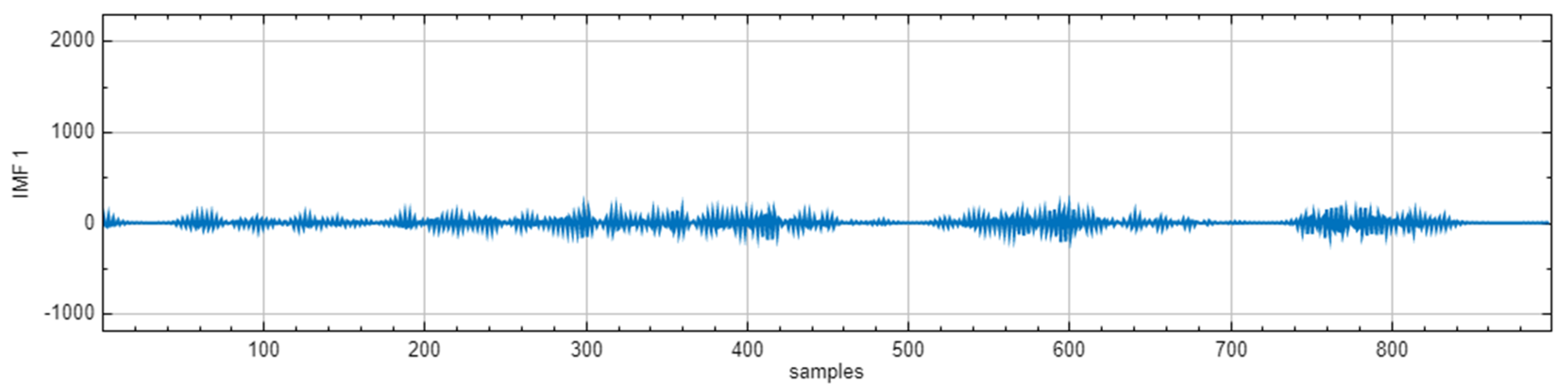
4.3. HESP Decomposition

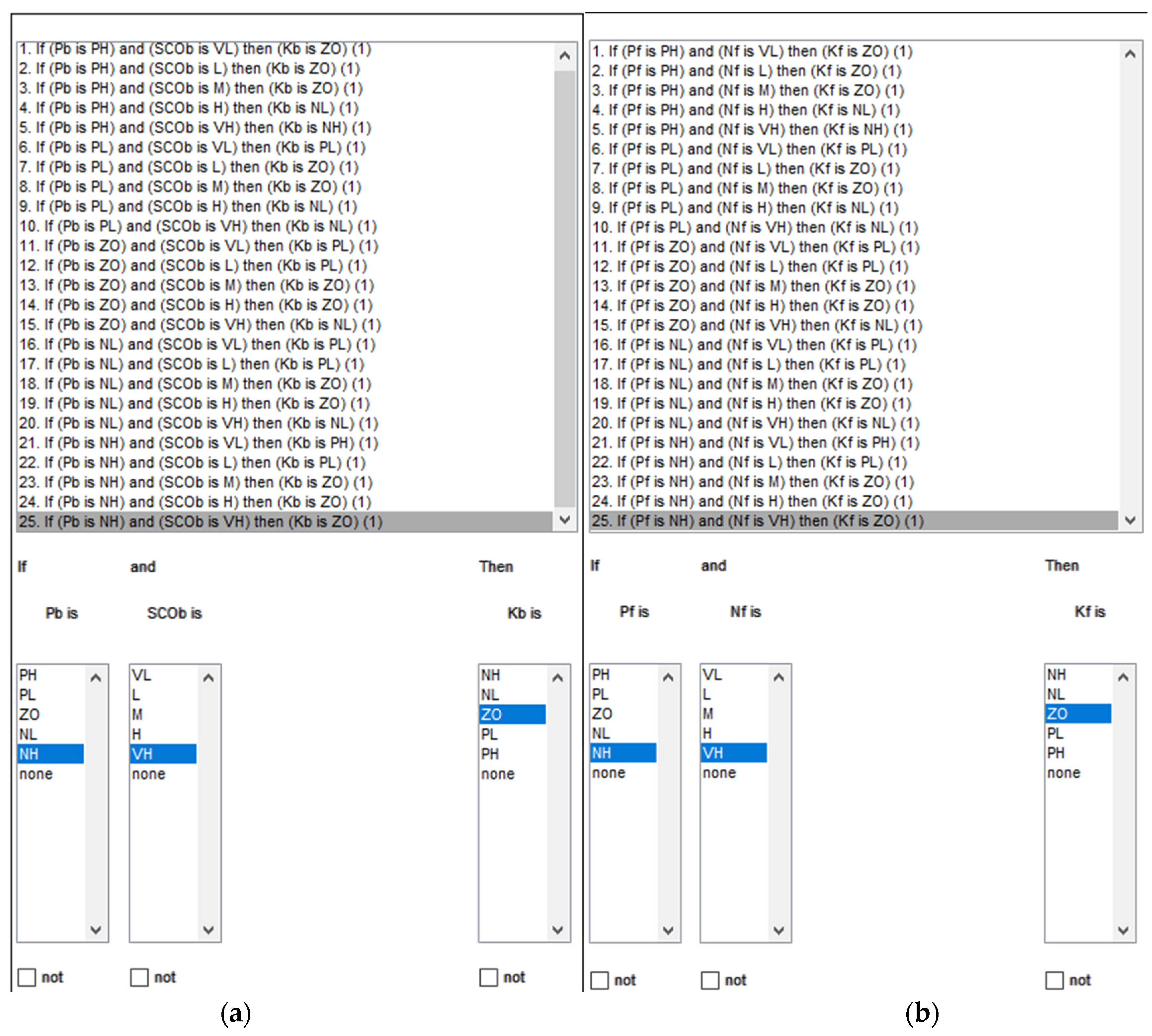
The HESS power was decomposed using the LSTM-optimized VMD method. The HESS power of IMF1-IMF6 after decomposition is shown below in Figure 10.

According to the preliminary power decomposition in Formula (19), IMF1-IMF3 was selected for low-frequency and IMF4-IMF6 for high-frequency decomposition.

4.4. Fuzzy Rule

The second revision to the fuzzy rule is shown in Figure 11.

4.5. Flywheel Energy Storage Power

According to the primary power distribution and the secondary power correction based on fuzzy reasoning, the power of the FESS is the high-frequency power component of the HESS; the reconstruction curve is shown in Figure 12. By comparing the curves optimized with LSTM to those without LSTM optimization, it can be seen that the power curves are all in the high-frequency range. The LSTM optimization method can better realize the fast charging–discharging of the flywheel and reduce the charging–discharging depth of the battery.

4.6. Battery Energy Storage Power

According to the primary power distribution and the secondary power correction based on fuzzy reasoning, the battery system power is the low-frequency power component of the HESS. Figure 13 shows the reconstruction curve, and Figure 14 shows the comparison of the depth of discharge (DOD) of the battery system. By comparing and analyzing the curves with LSTM optimization to those without LSTM optimization, it can be seen that the low-frequency power curve with LSTM optimization has less fluctuation, and the depth of charge–discharge is shallower. This avoids the overcharge and over discharge of the battery, delays the attenuation of the battery system, and prolongs the service life.

4.7. Discussion

The wind power, grid-connected power, flywheel power, and battery power were integrated into a chart, as shown in Figure 15.

From the above curve and the comparative analysis as shown in

Table 3. Comparison of methods and advantages.

References	Method	Advantage
		Smoothing Wind Power Fluctuations	SOC Constraint	DOD
Method of this paper	VMD+LSTM	Yes	Yes	Reduce DOD of BESS
Reference [30]	VMD	Yes	Yes	Reduce DOD of supercapacitor
Reference [32]	VMD+GWO (gray wolf optimization)	Yes	Yes	NO
Reference [33]	Wavelet packet decomposition	Yes	Yes	NO

, the following can be seen:

(1)

The power curve of the FESS fluctuates greatly, and the charge–discharge frequency is high, which meets the requirements of power-type energy storage;

(2)

The power curve of the BESS fluctuates less, and the charge–discharge frequency is low, which meets the requirements of energy storage;

(3)

The fluctuation of the grid-connected power curve is very small, which realizes the suppression of power fluctuation;

(4)

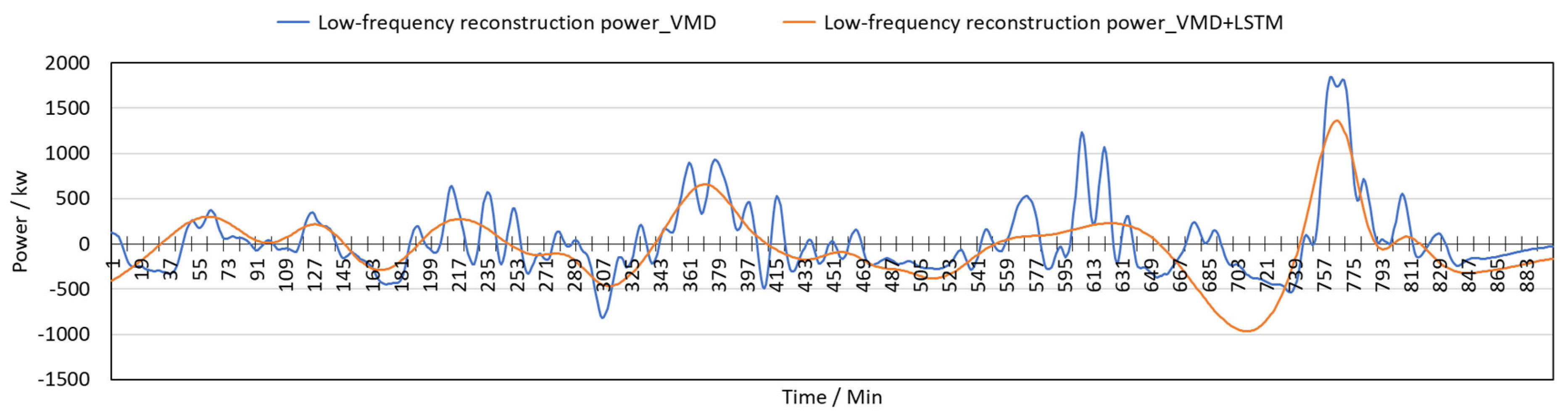
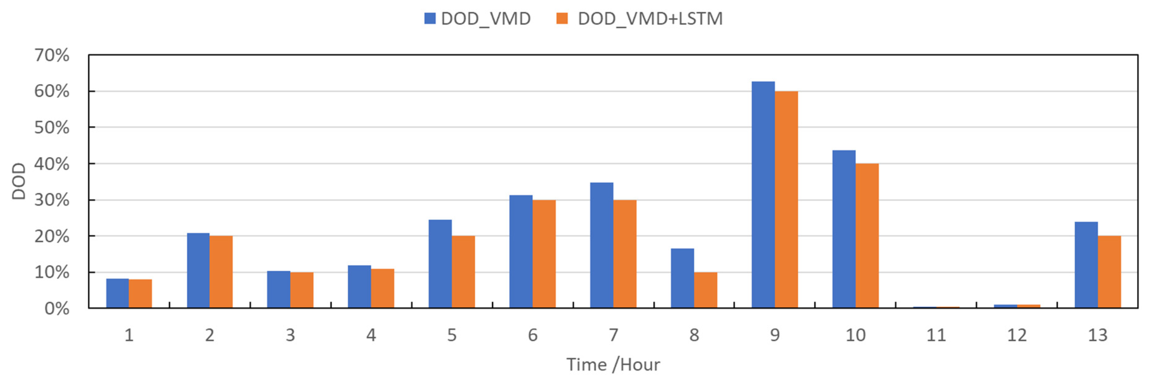
The low-frequency component of battery energy storage reconstructed using the LSTM-optimized VMD decomposition method has the advantage of extending the life of lithium battery systems. The depth of charge–discharge is shallower, which avoids the overcharge and over discharge of the battery, delays the attenuation of the battery system, and prolongs the service life.

5. Conclusions

In this paper, a hybrid flywheel–BESS based on optimal variational mode decomposition is proposed to smooth out wind power fluctuations. Firstly, the grid-connected power and charging–discharging power of the HESS were determined using the sliding average algorithm, and the HESP was decomposed using the LSTM-optimized VMD algorithm. Then, the power of the HESS was modified according to the rules formulated by fuzzy control. Finally, the feasibility and superiority of the proposed method were verified by a simulation example. The method proposed in this paper provides a reference for HESP configurations and control strategies.

Although the proposed method has certain feasibility and superiority, there are still many shortcomings in this paper:

(1)

This paper lacks the study of a wind power generation model, so this would be the next step;

(2)

We only used LSTM to optimize VMD; the next step will be to try to use other algorithms for optimization and to carry out comparative research.

References

1. Shi, W.; Bai, H.; Qu, J. Technology Trend and Development Suggestions for Wind Power Efficient Utilization in China. Strateg. Study CAE 2018, 20, 51–57. [Google Scholar] [CrossRef]
2. Xie, X.; Ma, N.; Liu, W.; Zhao, W.; Xu, P.; Li, H. Functions of Energy Storage in Renewable Energy Dominated Power Systems: Review and Prospect. Proc. CSEE 2023, 43, 158–169. [Google Scholar] [CrossRef]
3. Bai, L.; Li, F.; Hu, Q.; Cui, H.; Fang, X. Application of battery-supercapacitor energy storage system for smoothing wind power output: An optimal coordinated control strategy. In Proceedings of the 2016 IEEE Power and Energy Society General Meeting (PESGM), Boston, MA, USA, 17–21 July 2016; pp. 1–5. [Google Scholar] [CrossRef]
4. Li, H.; Zhang, Y.; Sun, W. Wind Power Fluctuation Smoothing Strategy with Generalized Energy Storage Under Wavelet Packet Decomposition. Power Syst. Technol. 2020, 44, 4495–4504. [Google Scholar] [CrossRef]
5. Li, Y.; Lin, X. Application of Hybrid Energy Storage System Based on SMES and BESS in Smoothing the Power Fluctuations of Wind Farms. High Volt. Eng. 2019, 45, 983–992. [Google Scholar] [CrossRef]
6. Liu, F.; Yang, X.; Shi, S. Hybrid energy storage scheduling based microgrid energy optimization under different timescales. Power Syst. Technol. 2014, 38, 3079–3087. [Google Scholar] [CrossRef]
7. Sang, B.; Wang, D.; Yang, B.; Ye, J.; Tao, Y. Optimal Allocation of Energy Storage System for Smoothing the Output Fluctuations of New Energy. Proc. CSEE 2014, 34, 3700–3706. [Google Scholar] [CrossRef]
8. Xiao, J.; Bai, L.; Lu, Z.; Wang, K. Method, implementation and application of energy storage system designing. Int. Trans. Electr. Energ. Syst. 2014, 24, 378–394. [Google Scholar] [CrossRef]
9. Han, X.; Chen, Y.; Zhang, H.; Chen, F. Application of hybrid energy storage technology based on wavelet packet decomposition in smoothing the fluctuations of wind power. Proc. CSEE 2013, 33, 8–13. [Google Scholar] [CrossRef]
10. Fu, J.; Chen, J.; Deng, H.; Sun, Z.; Zhang, B. Control strategy of hybrid energy storage system for mitigating wind power fluctuations. Electr. Meas. Instrum. 2020, 57, 94–100. [Google Scholar] [CrossRef]
11. Liu, Q.; Hu, Z.; Zhou, Y.; Lv, P.; Wang, J. Short-term Wind Power Fore-casting Based on CEEMD and random Forest Algorithm. Smart Power 2019, 47, 71–76. [Google Scholar]
12. Sun, C.; Yuan, Y.; Choi, S.S.; Li, M.; Zhang, X.; Cao, Y. Capacity optimization of hybrid energy storage systems in microgrid using empirical mode decom-position and neural network. Autom. Electr. Power Syst. 2015, 39, 19–26. [Google Scholar]
13. Zhang, Q.; Li, X.; Yang, M.; Cao, Y.; Li, P. Capacity determination of hybrid energy storage system for smoothing wind power fluctuation with maxi-mum net benefit. Trans. China Electrotech. Soc. 2016, 31, 40–48. [Google Scholar] [CrossRef]
14. Tang, J.; Zhu, J.; Li, Y.; Zuo, J.; Ma, J.; Chen, C. VMD based mode identification for broad-band oscillation in power system. Power Syst. Prot. Control 2019, 47, 7–14. [Google Scholar] [CrossRef]
15. Guo, X.; Li, L.; Cheng, Z.; Wu, L. Frequency and Voltage Modulation Control Strategy for Hybrid Energy Storage Device in Wind Power Island Mode. Power Syst. Clean Energy 2019, 35, 95–102. [Google Scholar]
16. Chen, H.; Lu, T.; Huang, J.; He, X.; Yu, K.; Sun, X.; Ma, X.; Huang, Z. An Improved VMD-LSTM Model for Time-Varying GNSS Time Series Prediction with Temporally Correlated Noise. Remote Sens. 2023, 15, 3694. [Google Scholar] [CrossRef]
17. Van, H.G.; Mosquera, C.; Napoles, G. A review on the long short-term memory model. Artif. Intell. Rev. 2020, 5, 5929–5955. [Google Scholar] [CrossRef]
18. Gasparin, A.; Lukovic, S.; Alippi, C. Deep learning for time series forecasting: The electric load case. CAAI Trans. Intell. Technol. 2022, 7, 5929–5955. [Google Scholar] [CrossRef]
19. Bashir, T.; Chen, H.; Tahir, M.F.; Zhu, L. Short term electricity load forecasting using hybrid prophet-LSTM model optimized by BPNN. Energy Rep. 2022, 8, 1678–1686. [Google Scholar] [CrossRef]
20. Lin, J.; Ma, J.; Zhu, J.; Cui, Y. Short-term load forecasting based on LSTM networks considering attention mechanism. Int. J. Electr. Power Energy Syst. 2022, 137, 107818. [Google Scholar] [CrossRef]
21. Li, J.; Song, Z.; Wang, X.; Wang, Y.; Jia, Y. A novel offshore wind farm typhoon wind speed prediction model based on PSOBi-LSTM improved by VMD. Energy 2022, 251, 123848. [Google Scholar] [CrossRef]
22. Yan, Y.; Wang, X.; Ren, F.; Shao, Z.; Tian, C. Wind speed prediction using a hybrid model of EEMD and LSTM considering seasonal features. Energy Rep. 2022, 8, 8965–8980. [Google Scholar] [CrossRef]
23. Yao, W.; Huang, P.; Jia, Z. Multidimensional LSTM networks to predict wind speed. In Proceedings of the 2018 37th Chinese Control Conference (CCC), Wuhan, China, 25–27 July 2018; pp. 7493–7497. [Google Scholar]
24. Lu, Z.; Yu, X.; Lu, C. Research on Sales Forecast of New Energy Vehicle Based on the Fusion Model of VMD and LSTM. J. Wuhan Univ. Technol. 2023, 45, 546–551. [Google Scholar]
25. Bing, Q.; Zhang, W.; Shen, F.; Hu, Y.; Gao, P.; Liu, D. Short-term traffic flow prediction based on variational model decomposition and LSTM. J. Chongqing Univ. Technol. 2023, 37, 169–177. [Google Scholar] [CrossRef]
26. Chen, L.; Shen, L.; Lu, F.; Ban, W. Forecast of Low-Sulfur Marine Fuel Price in Zhoushan Port Based on VMD-LSTM. J. Zhejiang Ocean Univ. 2023, 42, 346–351. [Google Scholar]
27. Han, L.; Zhang, R.; Wang, X.; Bao, A.; Jing, H. Multi-Step Wind Power Forecast Based on VMD-LSTM. IET Renew. Power Gener. 2019, 13, 1690–1700. [Google Scholar] [CrossRef]
28. Lu, J.; Zhang, Q.; Yang, Z.; Tu, M.; Lu, J.; Peng, H. Short-term load forecasting method based on CNN-LSTM hybrid neural network model. Autom. Electr. Power Syst. 2019, 43, 131–137. [Google Scholar] [CrossRef]
29. Zhang, T.; Tang, Z.; Wu, J.; Du, X.; Chen, K. Short Term Electricity Price Forecasting Using a New Hybrid Model Based on Two-Layer Decomposition Technique and Ensemble Learning. Electr. Power Syst. Res. 2022, 205, 107762. [Google Scholar] [CrossRef]
30. Jiao, D.; Chen, J.; Fang, Y.; Fu, J.; Deng, H.; Zhang, B. Control strategy of hybrid energy storage for suppressing fluctuation of wind power output based on variational mode decomposition. Electr. Meas. Instrum. 2021, 58, 14–19. [Google Scholar]
31. Gao, J.; Yang, D.; Wang, S.; Li, Z.; Wang, L.; Wang, K. State of health estimation of lithium-ion batteries based on Mixers-bidirectional temporal convolutional neural network. J. Storage 2023, 73, 109248. [Google Scholar] [CrossRef]
32. Du, G.; Chen, J.; Gao, L. Strategy of hybrid energy storage for wind power fluctuation smoothing based on optimized variational mode decomposition. Mod. Electron. Tech. 2023, 46, 1–7. [Google Scholar] [CrossRef]
33. Yuan, M.; Tian, L.; Jiang, T.; Hu, R.; Cui, X. Research on the capacity configuration of the “flywheel + lithium battery” hybrid energy storage system that assists the wind farm to perform a frequency modulation. J. Phys. Conf. Ser. 2022, 2260, 012026. [Google Scholar] [CrossRef]
Figure 1. Structure diagram of HESS.
Electronics 13 01362 g001
Figure 2. Flow chart of VMD algorithm.
Electronics 13 01362 g002
Figure 3. Flow chart of VMD algorithm.
Electronics 13 01362 g003
Figure 4. Flow chart of LSTM-optimized VMD algorithm.
Electronics 13 01362 g004
Figure 5. Power distribution diagram.
Electronics 13 01362 g005
Figure 6. Fuzzy control flow chart.
Electronics 13 01362 g006
Figure 7. Power distribution flow chart of HESS.
Electronics 13 01362 g007
Figure 8. Wind power curve.
Electronics 13 01362 g008
Figure 9. Curves of grid-connected and HESS power.
Electronics 13 01362 g009
Figure 10. HESP VMD decomposition curve.
Electronics 13 01362 g010aElectronics 13 01362 g010b
Figure 11. Fuzzy rules of (a) BESS and (b) FESS.
Electronics 13 01362 g011
Figure 12. Reconstruction curve of FESS.
Electronics 13 01362 g012
Figure 13. Reconstruction curve of BESS.
Electronics 13 01362 g013
Figure 14. BESS DOD curve.
Electronics 13 01362 g014
Figure 15. HESS power curve.
Electronics 13 01362 g015