1. Introduction
Steel is an alloy composed of iron and carbon, known for its high ductility, toughness, and strength [
1]. As a result, steel is widely utilized in modern industrial production, construction, and various other sectors. With the rapid advancement of modern industry, there is a growing demand for steel in our daily lives. However, steel materials are often susceptible to adverse effects during the production process, resulting in surface defects such as scratches and cracks. These defects compromise the physical structure of steel, significantly impacting the quality of the material. If steel materials with defects are used in the construction of buildings, automotive components, aircraft, and other engineering projects, it may even increase the risk of accidents. In the early stages, traditional steel surface defect identification relied mainly on manual visual inspection, which was a time-consuming and highly experiential task. It not only had low efficiency but also made it difficult to ensure consistency in identification quality.
It is worth noting that in recent years, machine learning and object detection technologies have made rapid progress, demonstrating tremendous potential in terms of target recognition speed, accuracy, automation, and sustainability. Especially in large-scale, high-speed, and high-precision target recognition tasks [
2], they have shown significant advantages over manual recognition. Object detection algorithms can be broadly classified into traditional methods and those grounded in deep learning.
Traditional object detection algorithms [
3] typically employ a sliding window search strategy, where a fixed-size window slides over the image, extracting features, and then using a classifier to determine if the window contains the target object. This approach involves a large amount of computation and time consumption during runtime, resulting in slow execution speed and limited accuracy, particularly for handling large images and large-scale datasets. The rapid advancement in deep learning has propelled deep learning-based object detection algorithms into the mainstream, marking substantial strides in the object detection domain. These algorithms can be broadly categorized into two-stage [
4] and one-stage [
5] approaches.
In 2014, R. Girshick et al. initially proposed the two-stage model region with CNN (RCNN) [
6]. This model uses selective search to extract object candidate boxes, then employs a convolutional neural network (CNN) to extract features, and finally uses a linear support vector machine for object classification. Two-stage models typically offer higher accuracy in object detection, and this design concept has profoundly influenced subsequent research. The Facebook team’s end-to-end object detection model based on Transformer, named DETR [
7], infers the relationships between objects and the global image background by providing a set of learned fixed small object queries, and directly generates the final prediction set in parallel. Xie et al. A new model [
8] was proposed, which combines CNN and Transformer for hybrid feature extraction to reduce model complexity and address the issue of Transformer’s lack of inductive bias. Joonhyeok Moon introduced the RoMP Transformer [
9], featuring rotation bounding boxes and a multi-layer feature pyramid. Compared to other contemporary neural networks, it demonstrates superior performance in terms of accuracy and computational speed. Sunkara presented a deep learning model called YOGA [
10], which includes a two-stage feature learning process and utilizes inexpensive linear transformations for feature map learning. These models exhibit several common characteristics. They demonstrate high accuracy and are capable of effectively handling variations in target size, deformation, and other changes, particularly showing improved detection performance for partially occluded, complex-shaped, or varying-sized objects. They have found wide applications in fields such as medical image analysis, security, and surveillance.
Simultaneously, one-stage detectors have also had a profound impact on the field of object detection. Since 2016, a series of one-stage detectors have emerged. R. Joseph proposed the milestone YOLO (You Only Look Once) algorithm [
11]. Subsequently, object detection algorithms based on the YOLO concept have been proposed. In 2018, R. Joseph introduced the YOLOv3 [
12] model based on YOLO, which utilizes multi-scale features for object detection, thereby improving the detection capability for objects of various sizes. Subsequently, in 2020, JOCHER G proposed the YOLOv5 [
13] model, which employs the Focus structure for efficient feature extraction and incorporates feature fusion operations using FPN+PAN. While these algorithms may have slightly lower accuracy compared to two-stage algorithms, they often exhibit higher operational speed and lower computational overhead. They are typically applied in scenarios that require real-time performance, such as autonomous driving or industrial assembly line operations.
With the continuous iteration of the YOLO network, it has gradually been applied to surface defect detection due to its good detection speed and accuracy. Guo et al. proposed an improved YOLOv5-based steel defect detection algorithm [
14]. They introduced the TRANS module, designed based on the Transformer architecture, into the network, facilitating feature fusion within the network. This integration enhances the detector’s capability to detect objects of varying scales through the implementation of multi-scale feature fusion structures, which merge features of different scales. Wang et al. proposed an improved algorithm based on YOLOv5s [
15]. In the model, they used coordinate attention, bidirectional feature pyramid network, and K-means algorithm to enhance the detection accuracy, and the experimental performance was significantly better than the original model. Zheng’s team proposed the EW-YOLOv7 defect detection model [
16]. By combining the Acmix attention mechanism with the GhostNetV2 module, they effectively optimized the defect detection performance. Ling Wang [
17] optimized the detection performance of YOLOv5 by using multi-scale detection blocks combined with an attention mechanism. Their model achieves a detection rate of 72% in mean Average Precision (mAP) for steel surface defects. Although these algorithms have improved the detection speed to some extent, there remains an issue of low overall detection accuracy. Due to the uncertainty associated with steel defects, it is common to encounter multiple defects of different scales and categories within a single image. Moreover, most real-world defect images exhibit blurry boundaries between the background and the defect segmentation, making it challenging to improve detection accuracy [
18].
In order to tackle the issue of low detection accuracy in current defect detection models, we compared different models and ultimately selected the YOLOv8n model structure as a reference. We introduced the Deformable ConvNets v2 (DCNV2) module, coordinate attention (CA) attention mechanism, Faster Block, and Ghost convolution (Ghost Conv) to reconstruct the network, proposing a more efficient and lightweight steel defect detection model.
Firstly, to improve the model’s feature extraction capability and generalization, we introduced the DCNV2 module in the feature extraction layer of the Backbone, which achieves adaptive receptive fields and enhances the model’s detection capability for complex objects. Secondly, to enable the model to more accurately focus on key feature information, and improve detection accuracy and speed, we optimized the CSPDarknet53 to two-stage FPN (C2f) module of the Backbone. This includes introducing the CA attention mechanism and using a more efficient Faster Block for feature extraction to reduce learning of unnecessary background information. Finally, to make the model faster in detection speed, we used Ghost Conv instead of regular convolution in the feature fusion network. With a certain receptive field maintained, this significantly reduces the computational burden of the model and more efficiently generates multiple feature maps, while reducing computational complexity while retaining redundant information. The above redesign results make the model more suitable for handling complex object detection tasks, optimizing the feature extraction, parameter quantity, and performance of the object detection model.
The primary contributions of this paper include the following:
We propose a new GDCP-YOLO model, which reduces redundant information extraction and achieves more effective steel surface defect detection by combining adaptive receptive fields and attention mechanisms.
We introduce the CA attention mechanism in the C2f module and use a more efficient Faster Block for feature extraction to reduce the model’s parameter quantity and improve its running speed.
We combine the coordinate attention which integrates CSPDarknet53 to two-stage FPN with Faster Block (CA_C2f_Faster) and Ghost Conv in our proposed model to achieve high accuracy while being lightweight. This branch model provides a lightweight improvement.
We conducted extensive comparative experiments to verify the performance optimization results of our proposed model. Additionally, we performed generalization experiments on the GDCP-YOLO model, providing a reference for its application in other detection fields.
The paper’s structure is outlined as follows: In
Section 2, we provide a brief overview of the reference model YOLOv8n, analyzing its inference process to provide a reference for subsequent innovations. In
Section 3, we analyze and discuss the new model proposed in this paper, introducing our innovative work. In
Section 4, we detail the datasets and corresponding experimental setups employed in our study. We compare, generalize, and perform ablation experiments on the proposed model to validate its effectiveness. In
Section 5, we summarize our work in this paper.
2. Structural Characteristics of the Reference Model
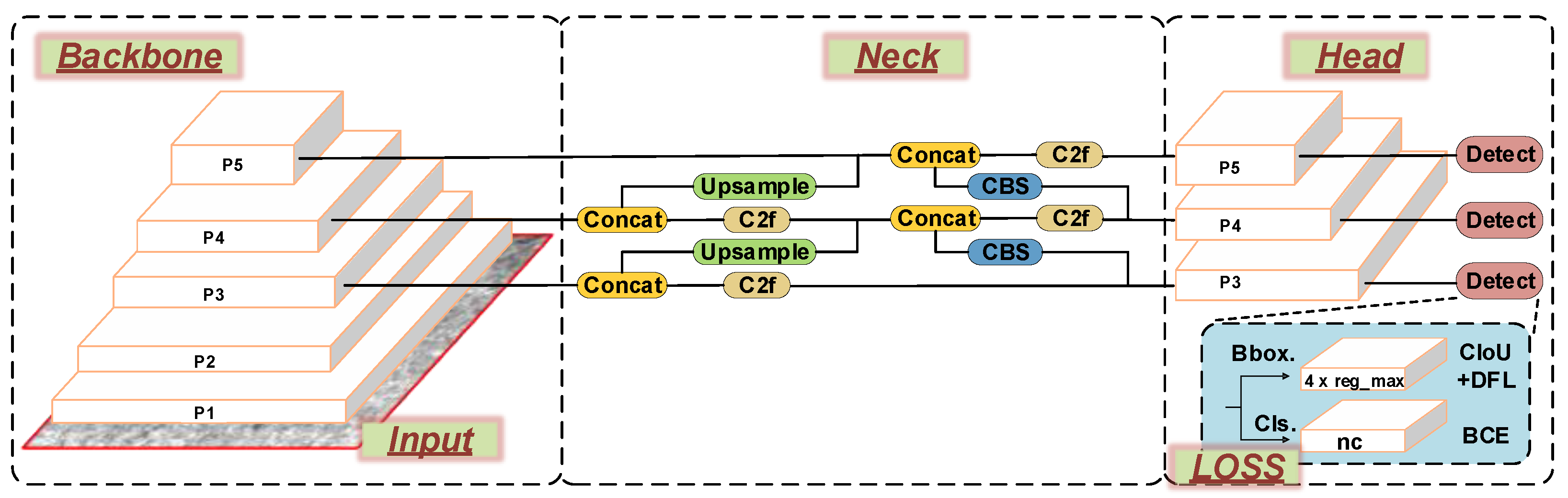
The YOLO algorithm reinterprets the object detection problem as a regression issue by predicting the position and class of objects on an image grid through a single convolutional neural network. This approach eliminates the traditional step of candidate box extraction, facilitating real-time object detection. YOLOv8n, a one-stage object detection algorithm, enhances the previous generations of the YOLO algorithm by accelerating operation, reducing model parameters, and improving recognition accuracy. The YOLOv8n network structure is illustrated in
Figure 1.
The input component is tasked with preprocessing the input image, which includes resizing it to a specific size, normalizing it, and converting it into a tensor format compatible with the neural network. Additionally, the input component incorporates data augmentation functionality. The Mosaic method merges multiple training images into a single large image, enabling simultaneous processing of multiple images in one forward pass. In the final 10 epochs of training, inspired by YOLOX, the Mosaic operation is deactivated.
The Backbone component, consisting of CBS (convolution, batch normalization, and activation function), C2f [
19], and Spatial Pyramid Pooling with Features (SPPF) [
13] modules, transforms the original image into a multi-scale, high-dimensional feature representation, forming multi-scale feature maps. In different stages of feature extraction, the output features are directly fed into the upsampling operation, eliminating the
convolution before upsampling in previous YOLO generations. The C2f module design mirrors the C3 module in preceding versions. It also adopts CSPNet and residual concepts [
20], dividing the network into two parts, each containing multiple residual blocks. However, compared to the original C3 module, it has more residual connections and includes additional split operations, eliminating the convolution operations in the branches, which enriches the feature information during gradient backpropagation. This division reduces model complexity while simultaneously enhancing feature extraction efficiency. The SPPF module transforms the originally parallel structure of Spatial Pyramid Pooling (SPP) into a serial structure. Before pooling, a convolution operation is performed on each region, and the convolution results are concatenated with the pooling results to form the output features. The module achieves a fusion of local and global information in feature maps through multi-scale pooling layers that preserve spatial information and adapt to different input sizes. The model employs the
SiLU activation function for its smoothness, non-linearity, and gradualness. It yields superior results compared to traditional Sigmoid and Tanh activation functions while avoiding potential gradient explosion issues associated with ReLU activation function. The SiLU activation function formula is as follows:
The Neck component comprises CBS, C2f, Upsample, and Concat modules, employing an FPN + PAN structure [
21]. This allows the network to fuse feature information of different scales simultaneously while preserving spatial information, better handling objects of varying sizes and improving object localization and classification accuracy.
The detect component adopts an anchor-free detection method, predicting the object’s center point and the distance from the center to each of its four edges directly. Furthermore, it replaces the IOU matching algorithm with the Task-Aligned Assigner matching strategy from the TOOD model [
22]. This strategy uses a high-order combination of classification scores and IoU to measure the degree of task alignment, helping the network dynamically prioritize high-quality anchors. The formula for the matching strategy is as follows:
Here,
s denotes the predicted box’s classification score,
u signifies the CIoU value [
23] between the predicted and ground truth boxes, and
and
are weight hyperparameters used to adjust the matching degree. The alignment degree can be measured by multiplying these two values. A
t value close to 1 indicates a higher degree of matching between the predicted box and the ground truth box, satisfying the conditions of a positive sample. The predicted boxes are sorted based on their matching degree with the ground truth box using
t, and then the top
K predicted boxes are selected as positive samples to enhance the model’s accuracy. When a predicted box matches multiple ground truth boxes, the one with the highest matching degree is retained.
The detect component separates the prediction of object position and class in the object detection task, enhancing the model’s flexibility and making it more adaptable for different object detection tasks and scenarios. The loss function used by the model comprises two components: classification and regression. The former uses binary cross-entropy (BCE) for loss calculation, while the latter uses Distribution Focal Loss (DFL) and CIoU Loss. The formula for the BCE loss is as follows:
In this context,
N stands for the batch size,
denotes the label value, and
signifies the predicted value of the model. The formula for
DFL is as follows:
Here,
y represents the label value, and
and
are the two closest label values to
y. The formula for
CIoU is as follows:
In these formulas, b and denote the center points of the predicted box and the ground truth box, represents the Euclidean distance between these two center points, c represents the diagonal distance of the minimum enclosing box that can contain both the predicted box and the ground truth box simultaneously, is a weight function, and v is used to measure aspect ratio consistency. During actual training, the model calculates total loss by weighting these three losses using a certain weight ratio.
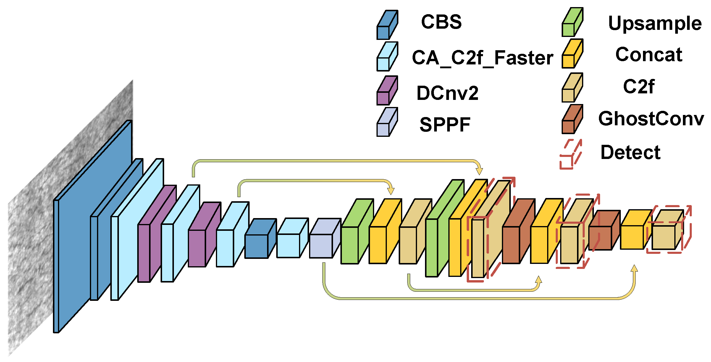
3. The GDCP-YOLO Framework: Enhancing Steel Surface Defect Detection
This study introduces a novel algorithm, GDCP-YOLO, specifically designed for steel surface defect detection. The model’s flowchart is provided in
Figure 2.
To enhance the object detection model’s performance and efficiency, we integrated various strategies into this new framework. Initially, we incorporated the DCNV2 module into the Backbone’s feature extraction layer, which serves to bolster the model’s feature extraction capability, facilitate adaptive receptive fields, and enhance spatial deformation processing and generalization abilities. Furthermore, we refined the C2f module of the Backbone by introducing the CA attention mechanism and employing a more efficient Faster Block for feature extraction.
The CA attention mechanism enables precise focus on critical feature channels, improving detection accuracy by minimizing irrelevant background information and reducing model parameters, thereby enhancing operational speed. Lastly, within the feature fusion network, we employed Ghost Conv instead of ordinary convolution to generate multiple feature maps more efficiently, further reducing the model’s parameter count while ensuring ample feature fusion and retaining redundant information. In summary, by incorporating the DCNV2 module, CA attention mechanism, Faster Block, and Ghost Conv, we have restructured the network to enhance feature extraction, reduce parameter count, and improve performance, enhancing its suitability for complex object detection tasks. The detailed parameter network structure of the GDCP-YOLO network is illustrated in
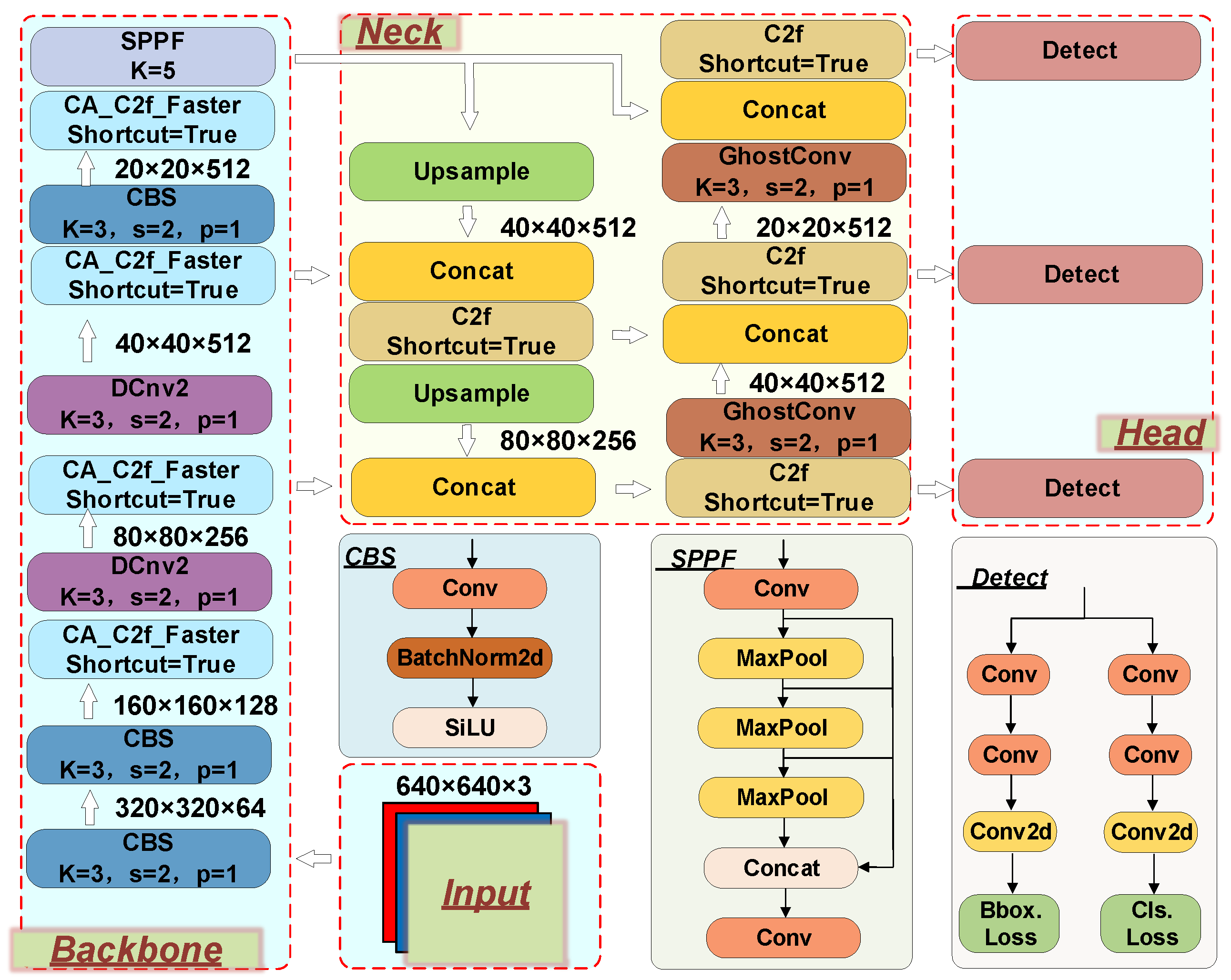
Figure 3, and its main features will be elaborated upon in subsequent sections.
3.1. DCNv2 Module
During the model training process, robust features often enable the model to learn more effective feature representations, thereby improving the model’s recognition capabilities. Therefore, selecting appropriate convolutions for feature extraction is particularly crucial. Ordinary convolution typically samples at fixed positions of the input feature map. This approach results in fixed weights of the convolution kernel, leading to a uniform receptive field size of the convolutional neural network when processing different position regions of the image. This is not optimal for deep convolutional neural networks as different positions may correspond to objects with varying scales or deformations. To tackle this issue, Zhu et al. developed DCNv2 [
24], which enhances the network’s adaptability to deformable targets through deformable convolutional layers and introduces an adjustment mechanism to optimize model offset learning.
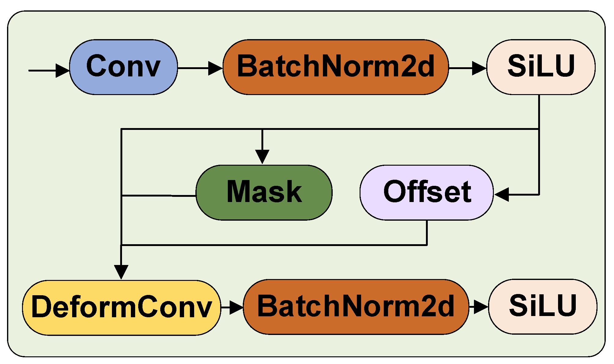
Drawing from the concept of DCNv2, we introduced the DCNV2 module into the key feature extraction layer of the Backbone. This incorporation enables adaptive adjustments in the size and shape of the receptive field through deformable convolution. This adaptation enables us to more effectively capture features that are close to the object’s shape and size, thereby enhancing the network’s generalization ability and improving its spatial deformation processing ability. As depicted in
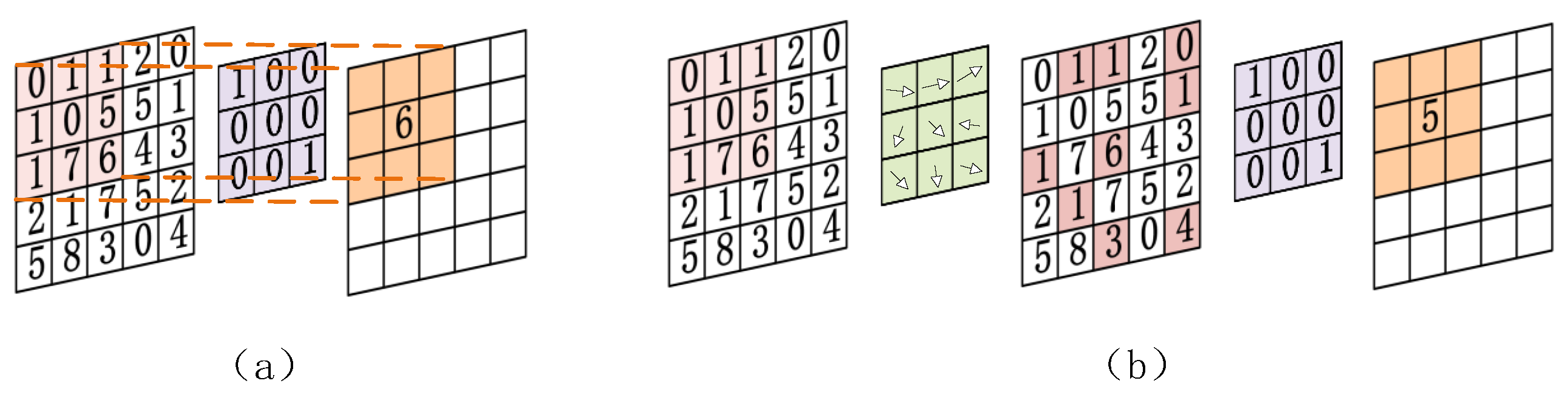
Figure 4, it shows the calculation process of ordinary convolution, which involves sliding a small convolution kernel on the input data and calculating the element-wise product sum of the convolution kernel and input data at each position. Its receptive field size is inherently fixed.
Figure 4b shows the calculation process of deformable convolution. By learning “offset” parameters, it allows offset operations on pixels in the input window, applies bilinear interpolation to generate sub-pixels, and then uses these sub-pixels instead of original pixels for convolution operation. The formula is as follows:
In this context, R represents the set of pixels in the current sliding window, w represents the convolution kernel, x represents the input image, represents the coordinates of the center point of the sliding window in the image, and represents the relative positions of other pixels in the sliding window to the center point. represents the learned offsets through Offset learning.
The specific details are illustrated in
Figure 5. The feature map first undergoes a 3 × 3 convolution for channel adjustment, followed by the BatchNorm layer and SiLU activation function. Next, the obtained features are input into three branches. One branch calculates the corresponding offsets for each pixel in the offset module, while another performs the corresponding Mask operation. The last branch, along with the calculated Mask parameters and Offset parameters, is input into the deformable convolution. Finally, the output goes through the BatchNorm layer and SiLU activation function.
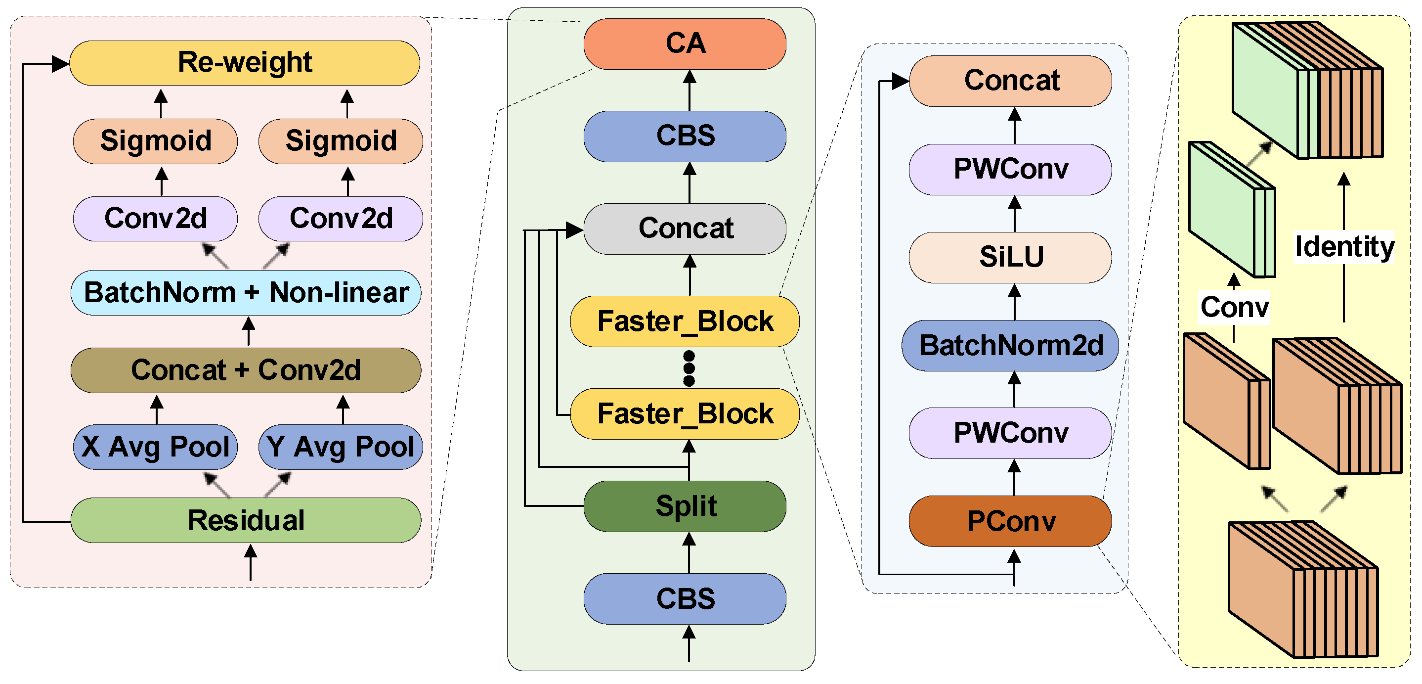
3.2. CA_C2f_Faster Module
In real-world scenarios, due to the influence of industrial production environments and detection equipment, capturing clear images of steel surfaces can be challenging. Some images may exhibit blurred detection targets and backgrounds, thereby complicating the extraction of steel surface defect features. To overcome this difficulty associated with feature extraction in steel defect detection models, we incorporated the CA attention mechanism [
25] into the C2f core feature extraction module of the Backbone. This mechanism encodes horizontal and vertical positional information into channel attention. The introduction of the attention module allows for the enhancement of feature-related channel information, adaptive learning of channel weights, and the model’s focus on more useful channel information, thereby improving the model’s ability to recognize and detect steel surface defects. The lightweight nature of the CA attention also enables the network to concentrate on large-scale positional information without significantly increasing computational load.
To tackle the issue of slow operation speed in the C2f module, we replaced the original Bottleneck with the recently developed Faster Block [
26]. The PConv within this block not only reduces computational burden but also extracts features more effectively than traditional deep convolution methods, making it suitable for multi-channel feature processing. This reduces model parameters and increases operational speed.
As shown in
Figure 6, once the feature map enters the module, we first use a CBS module to adjust the number of channels in the feature map to meet the model requirements. Then, we split the feature map using the split operation, introducing more branches and cross-layer connections to enhance the model’s gradient flow, promote information flow, and improve model performance. After splitting, we use the Faster Block for more comprehensive feature extraction on a portion of the feature map.
The Faster Block is primarily constructed using operations such as Pconv, PWconv, and normalization. In the Faster Block, we first use Pconv convolution for channel feature extraction. We use traditional convolution on only one-fourth of the input channels to extract spatial features, while the rest of the channels remain unchanged. To maximize information utilization across all channels, we add a point-wise convolution layer after PConv. This layer enables feature information to flow through all channels, ensuring that the model does not lose critical information while reducing redundant computations. For subsequent operations, batch normalization is used instead of other methods for faster inference. For activation layers, we select the SiLU activation function commonly used in YOLO to adapt to the entire model based on experience.
In CA attention, to avoid compressing spatial information into channels entirely, we do not use global average pooling. Instead, we decompose global pooling into encoding operations of two one-dimensional vectors. During the operation, we utilize two pooling kernels to process the channels separately along the horizontal and vertical directions. Their computational formulas are shown as follows:
We connect the feature maps generated by the two equations above and use a
convolution, normalization operation, and activation function for feature transformation. The specific process is as follows:
Then, we apply
convolutions and normalization operations to adjust the feature dimensions of tensors
and
, resulting in tensors
and
, respectively.
As shown in Equation (
13), we then apply the Sigmoid activation function to expand the obtained tensors
and
, which serve as attention weights. Finally, we multiply tensor
with the horizontal attention weight tensor
and the vertical attention weight tensor
at the corresponding coordinates in the
C channel. This calculation is used to compute the output of the coordinate attention block.
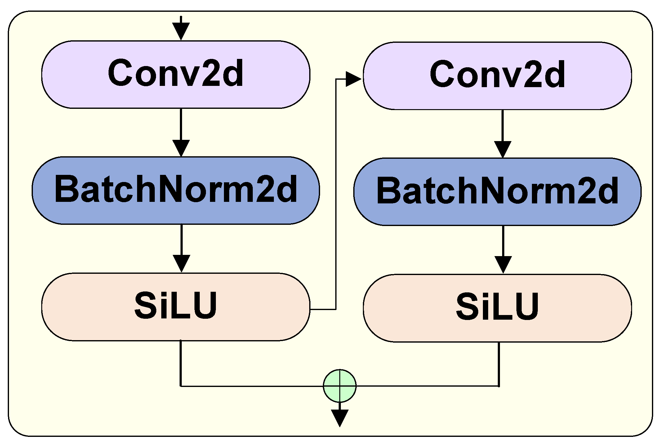
3.3. Ghost Conv
In actual industrial production, we receive a large number of images of steel surfaces. In order to efficiently process a large number of photos, the detection speed of the model is crucial. We typically enhance the model’s speed by reducing redundant computations. Traditional convolutions often extract redundant features, which can heavily impact memory usage and slow down model performance. In order to improve the model’s computational speed, we introduce the Ghost Module [
27] proposed by Huawei Noah’s Ark Lab, which can achieve the same effect as traditional convolutions with fewer computations.
As illustrated in
Figure 7, Ghost Conv decomposes a standard convolutional layer into two parts: a core convolution and an auxiliary convolution. These two convolutional layers learn primary and secondary features, respectively. The input feature map first passes through an auxiliary convolution with a kernel size of
. After the convolution operation, the number of channels is adjusted to half of the expected output channels, followed by a BatchNorm layer and SiLU activation function. Then, the obtained features are input into two branches, one of which passes through the main convolution with a
kernel, followed by a BatchNorm layer and SiLU activation function to obtain features. Finally, by stacking the outputs of the main and auxiliary convolutions, we obtain the final feature map. By using Ghost Conv, we reduce computational burden and eliminate redundant computations caused by traditional convolution operations without reducing accuracy, thereby reducing the number of model parameters.
4. Experimentation and Analysis of Results
4.1. Dataset
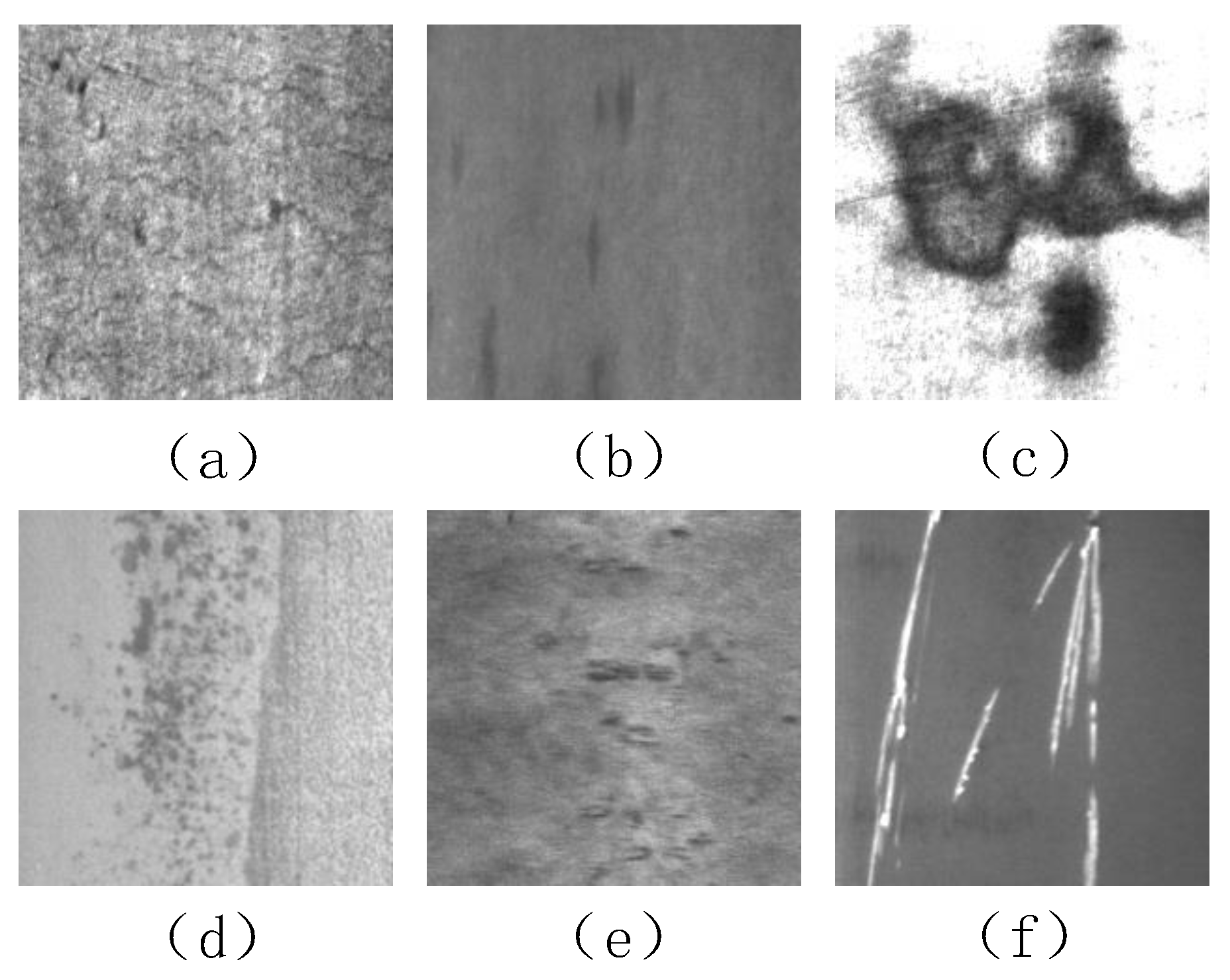
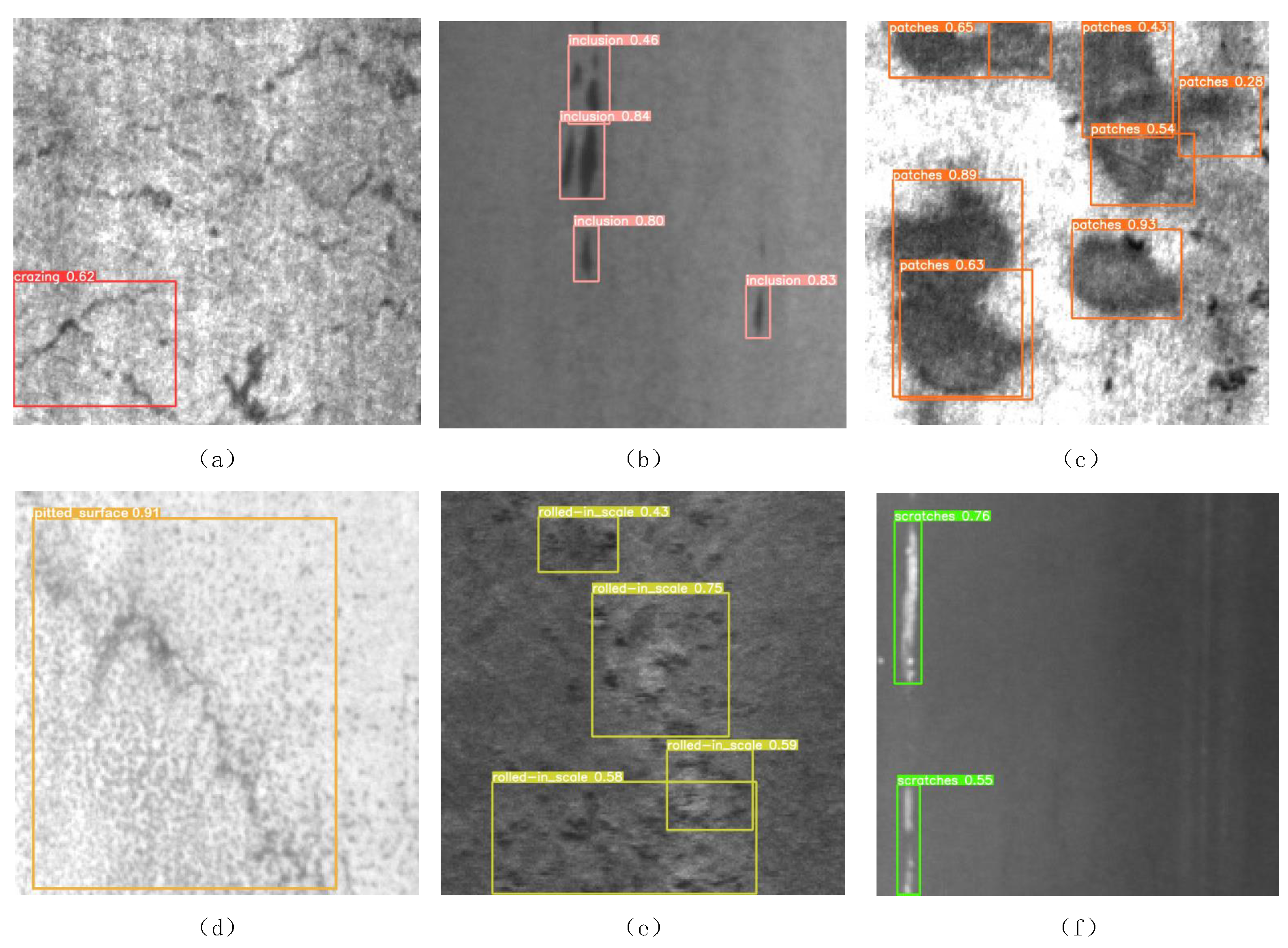
The NEU-DET steel surface defect dataset [
28], released by Northeastern University, was employed for this study. Due to the inaccurate annotation and low pixel quality of the crazing defect in this dataset, coupled with blurry backgrounds, the detection process poses certain challenges. It comprises 1800 grayscale images, each representing one of six typical surface defects found on hot-rolled steel strips: crazing (CR), inclusion (IN), patches (PA), pitted surface (PS), rolled-in scale (RS), and scratches (SC). Each defect category is represented by 300 images. The dataset includes annotations indicating the defect category and location in each image, as illustrated in
Figure 8.
After obtaining the raw dataset, we preprocessed the labels by converting the original XML labels into TXT format to suit our model’s requirements. The dataset was randomly divided into a 6:2:2 ratio, allocating 1040 images to the training set, 374 to the validation set, and the remaining 386 for model testing.
Table 1 presents the quantity of images and labels for each defect category in the training dataset.
4.2. Experimental Environment and Parameter Settings
The experiment utilized the hardware setup and key software settings detailed in
Table 2. This included setting the initial learning rate to 0.01, with a momentum parameter of 0.937 and weight decay of 0.0005. Stochastic Gradient Descent was employed as the optimizer, with a training duration of 300 epochs, a batch size of 16, and images resized to 640 × 640 pixels.
4.3. Evaluation Metrics
Object detection involves object classification and localization. The model’s performance was assessed using three main metrics: detection accuracy, detection speed, and model parameter count. Detection accuracy was assessed using mAP@0.5 and mAP@0.5:0.95 across the entire network model. Frames per second (FPS) were used to evaluate detection speed.
Average Precision (AP) gauges the correlation between precision and recall at various thresholds and is used to evaluate the model’s performance. The calculation of precision and recall is outlined in Equations (
14) and (
15).
True Positives (
TP) are instances where the model correctly identifies positive samples. False Positives (
FP) occur when negative samples are incorrectly labeled as positive, while False Negatives (
FN) are positive samples wrongly classified as negative. Equation (
16) depicts the Precision–Recall curve, where Precision (P) is on the vertical axis and Recall (
R) is on the horizontal axis. The area under the curve indicates the
AP.
In scenarios involving multi-category datasets, we calculate the
AP for each category independently, sum these
AP values, and then divide by the total number of categories (
n) to derive the mean Average Precision (
mAP) for all object detection categories.
FPS represents the model’s processing speed in terms of the number of images it handles per second. A higher FPS value indicates a faster processing rate.
4.4. Model Training
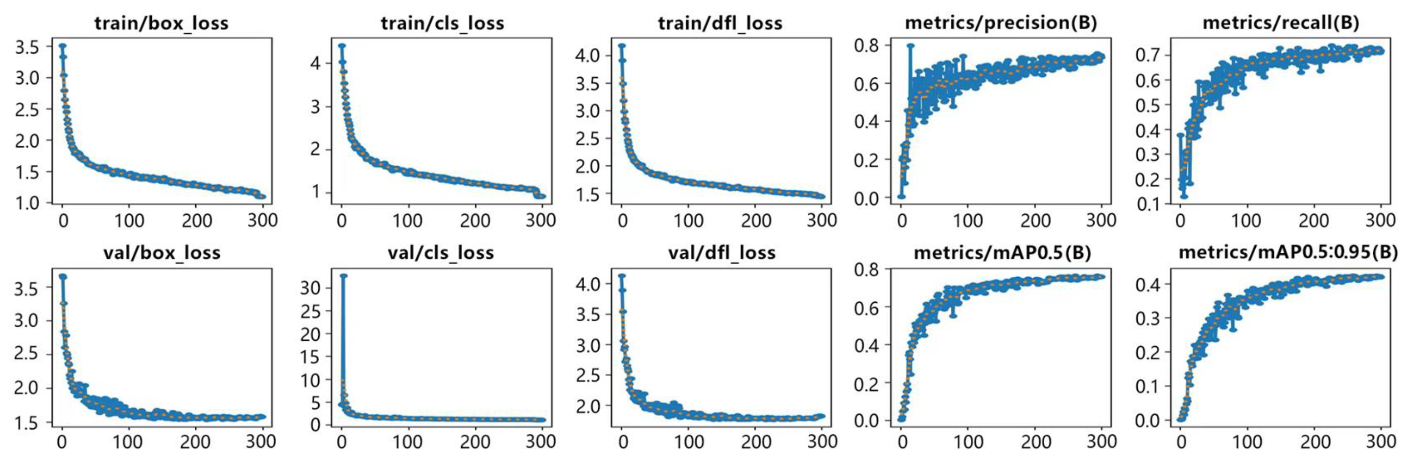
Tensorboard was used during training to monitor and record the model’s loss curve on datasets. As depicted in
Figure 9, both training and validation losses consistently decrease with the increase in the number of training iterations, indicating continuous learning and improvement of detection performance by the model.
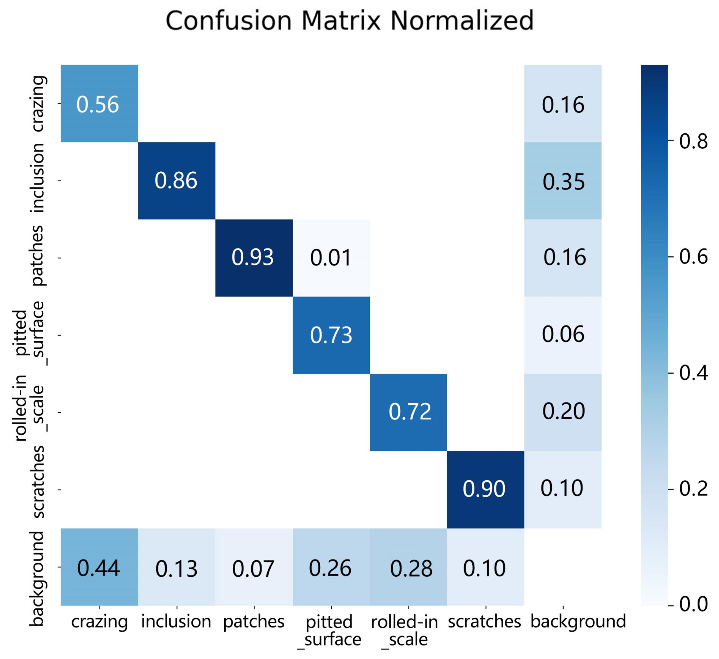
Post-training, the trained model was applied to the validation set, and the evaluation results are depicted in
Figure 10. The model demonstrated significantly higher detection accuracy for inclusion, patches, and scratches compared to the other three defect categories. This could be attributed to a higher number of labels for inclusion and patches in the training set, facilitating more comprehensive feature representation learning during model training. For scratches, the distinct contrast between its features and the background may have facilitated good feature learning despite limited labels.
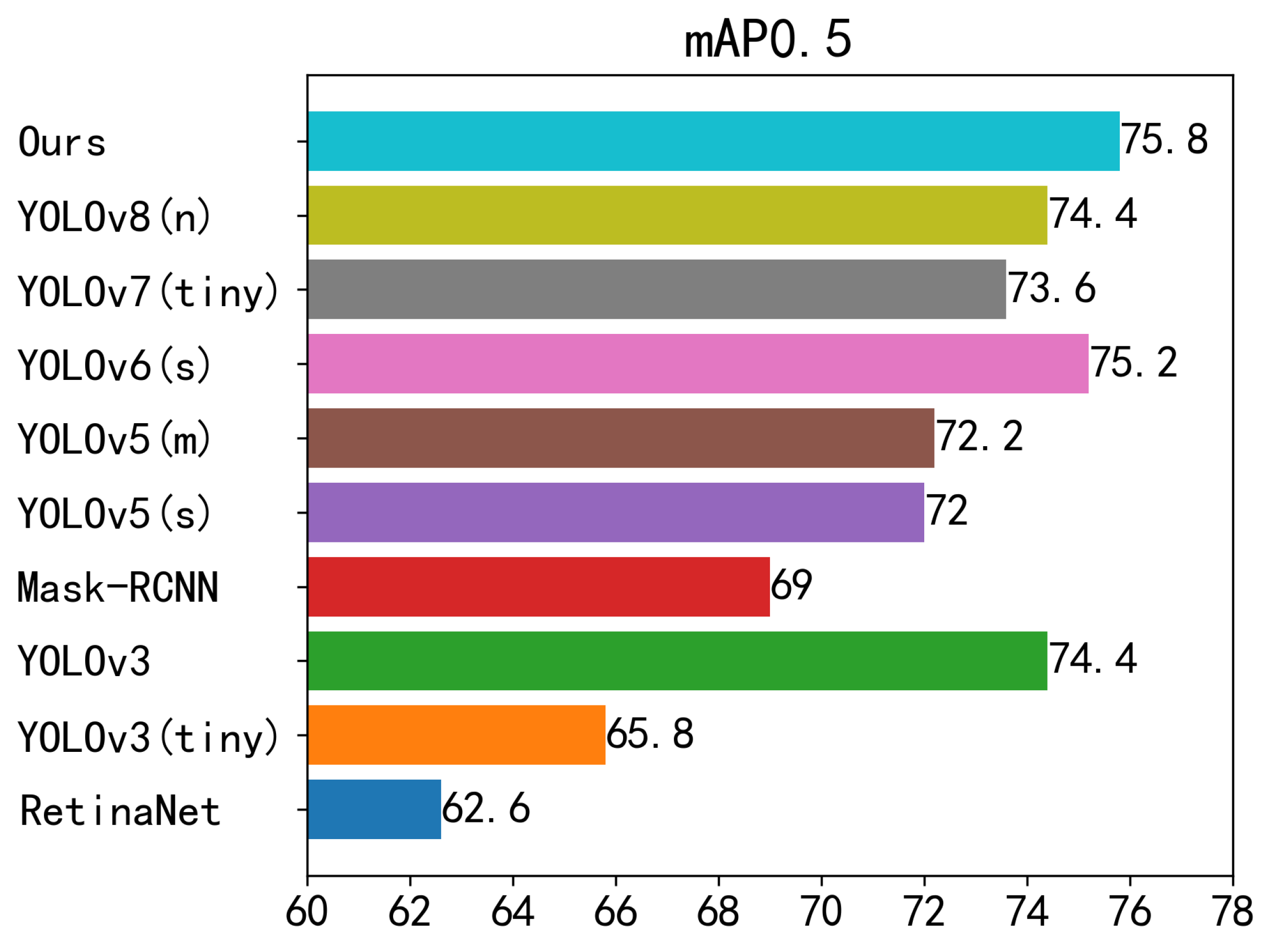
4.5. Comparative Experiments and Results
Assessing the effectiveness of our proposed algorithm, we conducted comparative experiments using the same dataset partition against RetinaNet [
29], YOLOv3 [
12], Mask-RCNN [
30], YOLOv5 [
13], YOLOv6, YOLOv7, and YOLOv8. Detailed results are depicted in
Figure 11.
The RetinaNet algorithm demonstrated a mean Average Precision (mAP) of only 62.6%, underscoring its limitations in accurately recognizing small targets within multiple defect categories. In contrast, the YOLOv3 (tiny) and YOLOv3 algorithms improved their mAP by 3.2% and 11.8%, respectively, indicating enhanced detection accuracy, particularly for the YOLOv3 algorithm when compared to RetinaNet. Since the YOLO model integrates unique multi-scale feature fusion prediction structures, it exhibits superior performance in detecting steel defects, which vary greatly in size.
Mask-RCNN adds a new Mask branch to the original RCNN model, aiding in model training and prediction. The addition of this branch enhances the model’s performance in detecting tasks with blurred backgrounds. This improvement results in a 6.4% increase in mAP compared to RetinaNet. YOLOv5 uses Mosaic data augmentation to preprocess initial images, allowing the model to learn more robust feature representations. Coupled with its adaptive anchor boxes, YOLOv5 demonstrates comprehensive improvements in detection across the dataset’s six categories. YOLOv5s and YOLOv5m achieve mAPs of 72% and 72.2%, respectively. YOLOv6 shows significant improvement in detecting crazing defects, achieving an mAP of 75.2%. Its use of a parameterized bakebone enhances model parallelism during runtime, and its novel loss function showcases good performance on imprecisely annotated data.
Our proposed algorithm improves by 1.4% and 2.2% compared to the original YOLOv8n and YOLO7 (tiny), respectively. Significant improvements are observed in detecting crazing, pitted surface, and rolled-in scale defects. By visually inspecting sample images of these defect categories, we notice prevalent blurriness, small, and densely clustered defects. Our CA_C2f_Faster module combines attention mechanisms with residual thinking for better feature extraction, possibly explaining why our model outperforms previous models.
These results suggest that our algorithm can recognize multiple defect categories on steel surfaces with higher accuracy than current mainstream detection algorithms.
To compare model detection speeds, we conducted tests on various algorithms under the same experimental conditions. As shown in
Figure 12, our proposed algorithm maintained a similar detection speed to the original YOLOv8n model, approximately double that of the RetinaNet algorithm, and essentially equivalent to YOLOv3 (tiny). This further validates our algorithm’s effectiveness in swiftly and accurately detecting steel surface defects.
In the earlier generations of YOLO, a significant number of convolution operations were used to enhance the model’s accuracy, resulting in slower inference speeds. YOLOv3 increased model complexity to improve accuracy, which led to an image detection efficiency of only 18.3% compared to our model within the same timeframe. While Mask-RCNN improved its runtime speed by 38.6 FPS compared to YOLOv3, its actual detection efficiency was only 28.3% of our model.
Starting from YOLOv5, designers began emphasizing the concept of lightweight models, reducing unnecessary convolution operations. This led to significantly higher detection speeds for YOLOv5s, YOLOv5m, and YOLOv6s, achieving 294.1 FPS, 163.9 FPS, and 277.8 FPS, respectively, although they still lagged behind our model’s 384.6 FPS.
We also conducted comparative experiments using the lightweight YOLOv7 (tiny) algorithm with the NEU-DET dataset. Due to the reduction of redundant computations during our model’s design phase, our proposed model surpassed YOLOv7 (tiny) in both detection accuracy and achieved detection speeds approximately 1.8 times faster.
Overall, our model performs exceptionally well in terms of running speed and demonstrates a significant advantage in accuracy over other mainstream models.
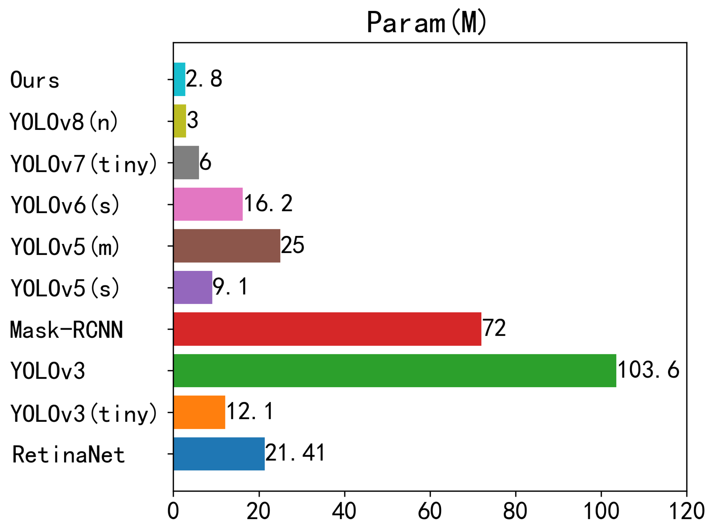
Figure 13 displays the number of parameters (Params) for each compared model, a metric reflecting the size of each model. The results reveal the following:
Our proposed algorithm holds a distinct advantage in parameter quantity compared to larger models like YOLOv3 and Mask-RCNN, with parameter quantities of only 2.7% and 3.8% of their original model parameter quantities, respectively.
Compared to medium-sized models such as YOLOv6s and YOLOv5m, our proposed algorithm reduces parameter quantity by approximately 13.4 M and 22.2 M, respectively.
Relative to smaller models like YOLOv7 (tiny), YOLOv5s, and YOLOv3 (tiny), our proposed algorithm possesses only half, one-third, and one-fourth of their parameter quantities, respectively. This suggests that our proposed algorithm is suitable for both GPUs and CPUs as well as certain low-computing power NPUs, demonstrating greater adaptability.
Compared to the original YOLOv8n algorithm, our parameter quantity has also been reduced by 7%.
These results indicate that we have struck a balance between speed, accuracy, and the number of parameters in detecting steel surface defects. Our proposed model demonstrates both practicality and advancement.
Figure 14 shows the detection results of various defect samples by category.
4.6. Generalization Experiments and Results
To reaffirm the efficacy of our proposed model, we performed generalization comparisons between the YOLOv8n model and our proposed algorithm, using the publicly available VOC2007 [
31] and GC10 datasets [
32]. The same experimental environment was maintained for these comparative experiments.
As depicted in
Table 3, our proposed algorithm outperformed the original YOLOv8n on the VOC2007 dataset, with a notable increase in mAP@0.5 of 2.1%. The mAP@0.5:0.95 remained fundamentally unchanged relative to the original model.
The algorithm demonstrated a significant enhancement over the original YOLOv8n on the GC10 dataset (
Table 4), with increases of 1.9% and 1.3% in mAP@ 0.5 and mAP@ 0.5:0.95, respectively. This affirms that our improved algorithm not only achieved progress on the NEU-DET dataset but also exhibited considerable improvement on publicly available datasets, indicating good generalization capability of the improved model.
4.7. Ablation Experiments and Results
To scrutinize the improvements offered by the three proposed enhancements to the network model, we undertook ablation experiments on the NEU-DET dataset using YOLOv8n as the baseline network (
Table 5). The experimental environment and parameter settings remained consistent.
Table 5 reveals that employing the CA_C2f_Faster module alone augmented the speed of the baseline network by 41.1 FPS and reduced the parameter quantity by 11.7%. This is primarily due to the employment of lightweight Pconv for feature extraction, combined with the CA attention module with fewer parameters and computations, effectively enhancing the model’s running speed and reducing its parameter quantity. The experiment discovered that combining the CA_C2f_Faster module with Ghost Conv further improved FPS and model parameter quantity, yielding optimal results among all experimental groups, with a speed of 439.8 FPS and a parameter quantity of 2.56M. Remarkably, its model accuracy also ranked second in the experiments, second only to our final model, revalidating the effectiveness of our designed CA_C2f_Faster in improving running speed and reducing model parameters.
Ultimately, the incorporation of the DCnv2 module led to peak accuracy. The model saw a 2.3% rise in recall rate and achieved an mAP@0.5 of 75.8%, surpassing the baseline model, and mAP@ 0.5:0.95 increased by 1.8%. This suggests that the DCnv2 module, which incorporates deformable convolutional thinking, is effective in capturing features of varying sizes and positions to learn richer semantic features. This makes the network model more comprehensive in detecting steel surface defects and improves its performance.


