
A Deterministic Chaos-Model-Based Gaussian Noise Generator

 , , , , and
Abstract
:1. Introduction
2. Materials and Methods
2.1. Central Limit Theorem
2.2. Basic Distributions
2.3. Measures of Similarity of Probability Density Functions
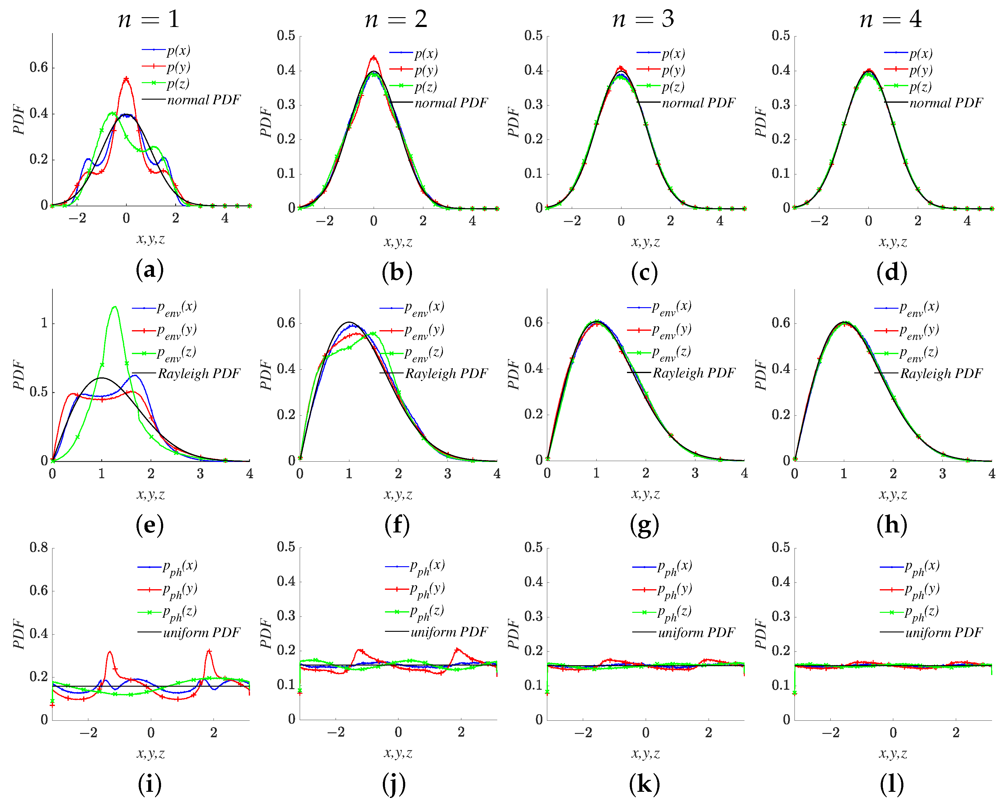
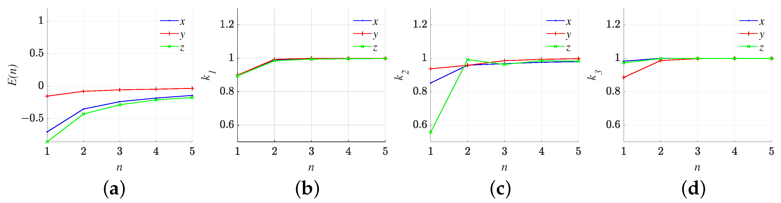
3. Properties of Sums of Chaotic Signals
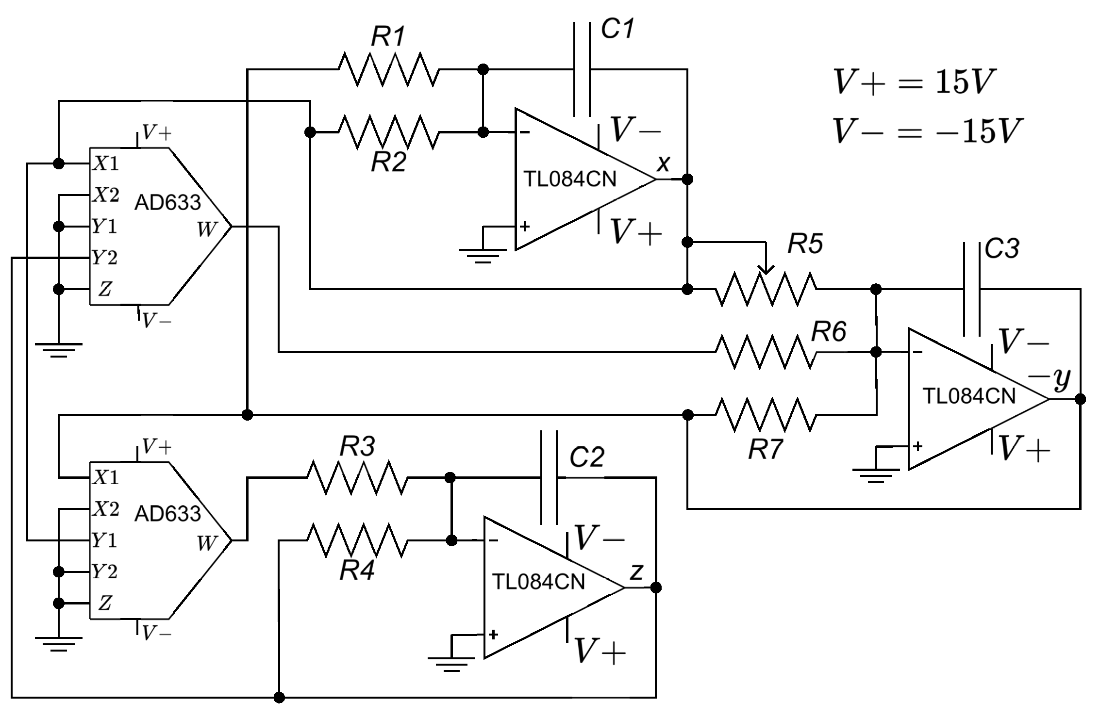
3.1. Chua’s Circuit
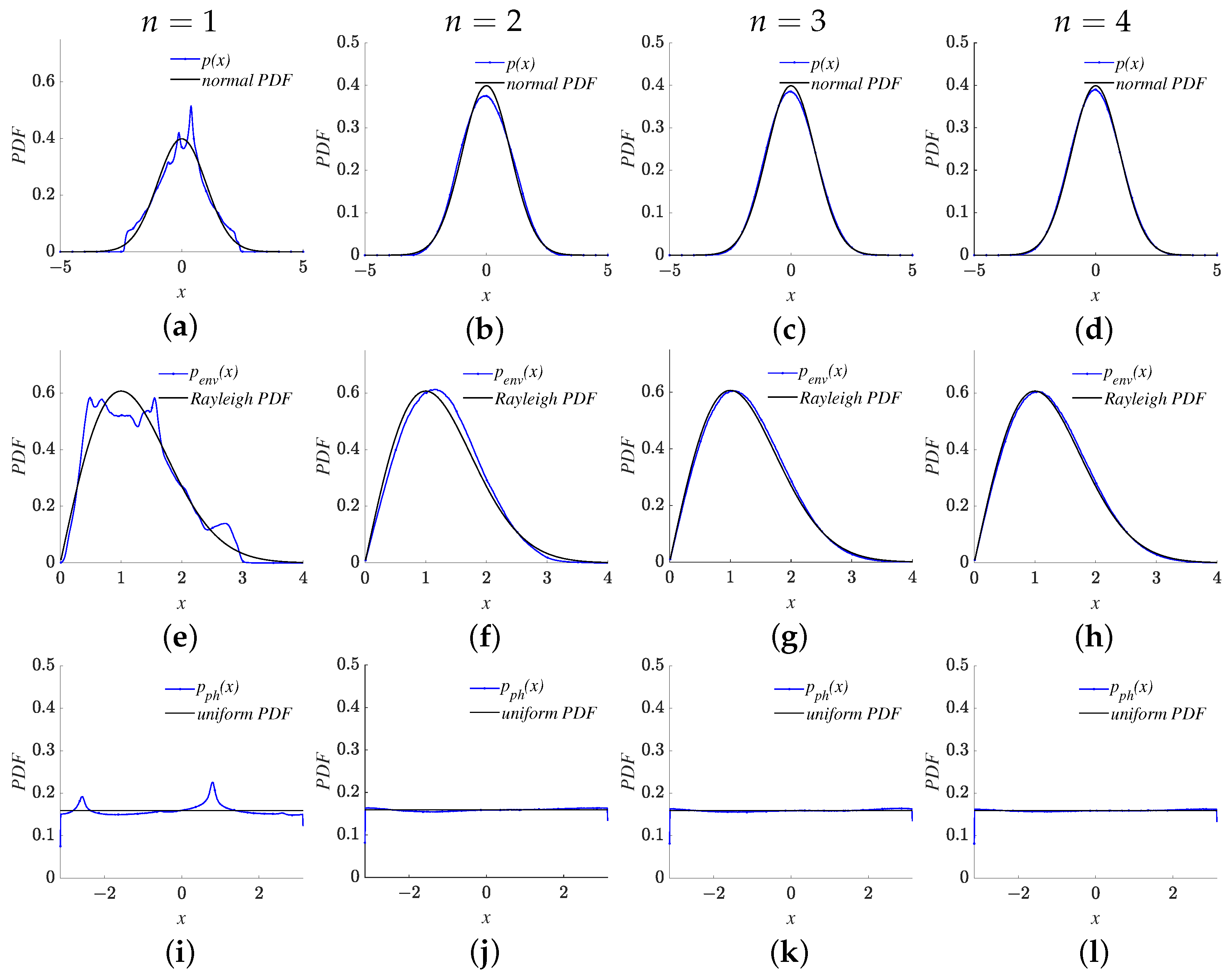
3.2. Lorenz System
4. Experimental Verification
4.1. Experiment with Chua’s Circuit
4.2. Experiment with a Lorenz System
5. Discussion and Conclusions
- i.
- Prioritize signals possessing symmetric probability density functions.
- ii.
- Minimize the excess kurtosis of the selected signals, ideally aiming for .
- iii.
- Ensure that all three entropy powers () of the original chaotic signal surpass a value of .
- i.
- Covert communication—there are approaches based on thermal noise or AI noise; therefore, our recommendation is to use artificial Gaussian-distributed chaotic signals for hidden communication;
- ii.
- Radio countermeasure purposes—the deterministic nature of chaotic systems can be used to reproduce and compensate for the influence of chaos in “friendly devices” and remains incomprehensible for “enemies”. This means that the same signal can be at least neutral for one device and harmful to others;
- iii.
- PRNG for cryptography purposes—a huge number of scientific studies are concerned with this question. By increasing the number of chaotic signals, we increase the keyspace of the encrypted information.
Author Contributions
Funding
Data Availability Statement
Conflicts of Interest
Appendix A

| Chaotic System | Output Variable | |||||
|---|---|---|---|---|---|---|
| Chua’s circuit [49] | ||||||
| x | −0.0116 | −1.6609 | 0.3626 | 0.4754 | 0.8435 | |
| y | −0.0028 | −0.1421 | 0.9039 | 0.9756 | 0.9980 | |
| z | 0.0084 | −1.1152 | 0.7541 | 0.8128 | 0.9056 | |
| where ; ; ; ; ; . | ||||||
| Pairwise sum of two signals | ||||||
| 0.0033 | −0.8287 | 0.7040 | 0.9349 | 0.9696 | ||
| 0.0029 | −0.0717 | 0.9961 | 0.9604 | 0.9989 | ||
| −0.0007 | −0.5581 | 0.9648 | 0.9976 | 0.9965 | ||
| Pairwise sum of three signals | ||||||
| −0.0059 | −0.5519 | 0.8741 | 0.8897 | 0.9873 | ||
| 0.0015 | −0.0367 | 0.9996 | 0.9893 | 0.9986 | ||
| 0.0089 | −0.3715 | 0.9901 | 0.9798 | 0.9987 | ||
| Pairwise sum of four signals | ||||||
| −0.0090 | −0.4088 | 0.9467 | 0.9783 | 0.9982 | ||
| 0.0009 | −0.0034 | 0.9998 | 0.9908 | 0.9985 | ||
| 0.0105 | −0.2700 | 0.9955 | 0.9907 | 0.9994 | ||
| Experiment with Chua’s circuit | ||||||
| y | −0.0518 | −0.4249 | 0.9437 | 0.9381 | 0.9950 | |
| 0.0339 | −0.3837 | 0.9897 | 0.9192 | 0.9986 | ||
| 0.0511 | −0.2393 | 0.9962 | 0.9629 | 0.9986 | ||
| 0.0420 | −0.1846 | 0.9979 | 0.9720 | 0.9985 | ||
| Chua’s circuit [49] | ||||||
| x | −0.0763 | −1.4807 | 0.5463 | 0.6532 | 0.9087 | |
| y | −0.0070 | −0.9334 | 0.8739 | 0.5006 | 0.9989 | |
| z | 0.0465 | −0.8164 | 0.8676 | 0.8860 | 0.9808 | |
| where ; ; ; ; ; . | ||||||
| Chaotic System | Output Variable | |||||
|---|---|---|---|---|---|---|
| Lorenz [53] | ||||||
| x | 0.0003 | −0.7093 | 0.8989 | 0.8535 | 0.9830 | |
| y | 0.0005 | −0.1573 | 0.9013 | 0.9368 | 0.8877 | |
| z | 0.2023 | −0.8499 | 0.8974 | 0.5618 | 0.9731 | |
| Pairwise sum of two signals | ||||||
| −0.0102 | −0.3529 | 0.9893 | 0.9587 | 0.9995 | ||
| −0.0103 | −0.0801 | 0.9938 | 0.9580 | 0.9865 | ||
| 0.0014 | −0.4291 | 0.9852 | 0.9921 | 0.9983 | ||
| Pairwise sum of three signals | ||||||
| −0.0053 | −0.2393 | 0.9966 | 0.9677 | 0.9989 | ||
| −0.0059 | −0.0570 | 0.9993 | 0.9857 | 0.9978 | ||
| 0.0397 | −0.2867 | 0.9946 | 0.9631 | 0.9994 | ||
| Pairwise sum of four signals | ||||||
| −0.0031 | −0.1840 | 0.9981 | 0.9759 | 0.9987 | ||
| −0.0040 | −0.0468 | 0.9997 | 0.9937 | 0.9999 | ||
| 0.0002 | −0.2122 | 0.9975 | 0.9852 | 0.9987 | ||
| Experiment with Lorenz system | ||||||
| x | 0.0131 | −0.5906 | 0.9292 | 0.8454 | 0.9606 | |
| 0.0150 | −0.1978 | 0.9937 | 0.9995 | 0.9976 | ||
| 0.0204 | −0.0523 | 0.9989 | 0.9996 | 0.9993 | ||
| 0.0246 | 0.0499 | 0.9995 | 0.9886 | 0.9996 | ||
| Lorenz [53] | ||||||
| x | −0.0034 | −0.9328 | 0.8961 | 0.7523 | 0.9649 | |
| y | −0.0038 | −0.3519 | 0.9801 | 0.9247 | 0.8355 | |
| z | 0.0821 | −0.4826 | 0.9736 | 0.7515 | 0.9786 | |
| Chaotic System | Output Variable | |||||
|---|---|---|---|---|---|---|
| Bhalekar and Gejji [56] | ||||||
| x | −0.4940 | −0.3912 | 0.8739 | 0.5924 | 0.9420 | |
| y | −0.0029 | −0.2152 | 0.9362 | 0.7205 | 0.7675 | |
| z | −0.0029 | −0.0071 | 0.9586 | 0.9157 | 0.6919 | |
| Chen and Lee [57] | ||||||
| x | −0.0009 | −1.3013 | 0.7086 | 0.2180 | 0.9371 | |
| y | 0.0027 | −0.7711 | 0.9037 | 0.3269 | 0.8813 | |
| z | 0.4027 | −0.6617 | 0.7847 | 0.5387 | 0.9838 | |
| Cheng et al. [58] | ||||||
| x | 0.0042 | −0.7241 | 0.8544 | 0.7317 | 0.9969 | |
| y | 0.0002 | −0.6388 | 0.9540 | 0.7494 | 0.9792 | |
| Colpitts chaotic oscillator [59,60] | ||||||
| x | −1.3378 | 1.5271 | 0.5924 | 0.7753 | 0.7510 | |
| y | −0.9897 | 0.0021 | 0.4836 | 0.6179 | 0.9102 | |
| z | 1.0142 | 0.3489 | 0.6171 | 0.9408 | 0.8144 | |
| where ; ; ; ; ; ; ; ; . | ||||||
| Dong et al. [61], | ||||||
| x | 1.3143 | 15.2455 | 0.1413 | 0.2982 | 0.7632 | |
| y | −1.5546 | 1.4611 | 0.1139 | 0.6076 | 0.7315 | |
| z | 1.6361 | 1.9200 | 0.0925 | 0.6168 | 0.7312 | |
| where , , , , , , , , , | ||||||
| Flux controlled memristor [62] | ||||||
| x | −0.0145 | 3.7663 | 0.6712 | 0.8624 | 0.9455 | |
| y | −0.0000 | 0.3748 | 0.8951 | 0.8874 | 0.9883 | |
| z | 0.0017 | 0.2822 | 0.8733 | 0.8835 | 0.9959 | |
| w | −0.0916 | −1.8739 | 0.1006 | 0.3087 | 0.6974 | |
| where ; ; ; ; ; ; ; . | ||||||
| Genesio and Tesi [63,64] | ||||||
| x | 0.1377 | −1.1867 | 0.6227 | 0.2463 | 0.9980 | |
| y | 0.3478 | −1.2245 | 0.5156 | 0.1004 | 0.9931 | |
| z | 0.1864 | −1.1514 | 0.6580 | 0.2095 | 0.9697 | |
| where ; ; . | ||||||
| Li et al. [65] | ||||||
| x | −0.0051 | −0.2485 | 0.7872 | 0.8415 | 0.8433 | |
| y | −0.0003 | −0.6939 | 0.8603 | 0.7182 | 0.9157 | |
| z | −0.0980 | −0.9221 | 0.8613 | 0.7934 | 0.9360 | |
| Li and Sprott [66] | ||||||
| x | 0.0023 | −0.2196 | 0.8567 | 0.9277 | 0.8624 | |
| y | −0.2622 | 0.1621 | 0.9575 | 0.9152 | 0.9130 | |
| z | 0.0094 | 0.3070 | 0.9607 | 0.5493 | 0.8597 | |
| Liu and Chen [67] | ||||||
| x | 0.0132 | 0.9226 | 0.9241 | 0.9580 | 0.7826 | |
| y | −0.0007 | 11.7760 | 0.3050 | 0.9763 | 0.5337 | |
| z | −0.0449 | 5.0172 | 0.5013 | 0.8873 | 0.7990 | |
| Lü and Chen [68] | ||||||
| x | −0.0002 | −0.4949 | 0.9266 | 0.8457 | 0.8685 | |
| y | −0.0006 | −0.3236 | 0.9422 | 0.9108 | 0.8483 | |
| z | 0.2535 | −0.3539 | 0.9408 | 0.7114 | 0.9495 | |
| Lü et al. [69,70] | ||||||
| x | 0.0113 | 0.2948 | 0.9342 | 0.8041 | 0.5401 | |
| y | −0.1063 | 41.3350 | 0.0006 | 0.1884 | 0.0019 | |
| z | −0.0601 | 23.7057 | 0.0011 | 0.6488 | 0.0110 | |
| Memristive circuit [12,71] | ||||||
| x | −0.8235 | 0.0391 | 0.7455 | 0.6689 | 0.9496 | |
| y | 0.4986 | 0.5598 | 0.8316 | 0.9146 | 0.8807 | |
| z | −0.8277 | −0.2585 | 0.6046 | 0.4188 | 0.9038 | |
| Özoǧuz et al. [72] | ||||||
| x | 0.0039 | −0.8260 | 0.8818 | 0.8230 | 0.9784 | |
| y | −0.0032 | −0.6363 | 0.9356 | 0.7480 | 0.9489 | |
| z | −0.0048 | −1.0010 | 0.8591 | 0.6947 | 0.9769 | |
| where . | ||||||
| Qi et al. [73] | ||||||
| x | −0.0313 | 0.6421 | 0.9562 | 0.8812 | 0.9000 | |
| y | 0.0158 | 0.9269 | 0.9554 | 0.9238 | 0.9044 | |
| z | 0.0375 | 4.1904 | 0.7527 | 0.8528 | 0.9239 | |
| Ring oscillating systems [74] | ||||||
| x | −0.0003 | −0.7734 | 0.8992 | 0.7333 | 0.9900 | |
| y | 0.0012 | −0.5155 | 0.9619 | 0.9643 | 0.9762 | |
| z | 0.0014 | −1.1498 | 0.7992 | 0.7124 | 0.9259 | |
| where ; ; ; . | ||||||
| Rössler [75] | ||||||
| x | 0.2261 | −0.7120 | 0.8709 | 0.5620 | 0.9958 | |
| y | −0.1768 | −0.8174 | 0.8565 | 0.5895 | 0.9958 | |
| z | 5.3359 | 31.4457 | 0.0007 | 0.1869 | 0.4920 | |
| Sprott [76], system A | ||||||
| x | 0.4457 | 0.1407 | 0.7233 | 0.8802 | 0.9472 | |
| y | 0.0004 | 0.6015 | 0.9336 | 0.8052 | 0.8718 | |
| z | −0.0003 | −0.7692 | 0.9357 | 0.5446 | 0.9792 | |
| Sprott [76], system B | ||||||
| x | −0.0854 | 0.6461 | 0.9488 | 0.9882 | 0.8560 | |
| y | −0.0859 | −0.4976 | 0.9265 | 0.7967 | 0.9309 | |
| z | 0.0550 | 1.0485 | 0.9573 | 0.9551 | 0.9124 | |
| Sprott [76], system C | ||||||
| x | −0.0285 | −0.1891 | 0.9670 | 0.9618 | 0.9479 | |
| y | −0.0333 | −0.9804 | 0.8582 | 0.8341 | 0.9715 | |
| z | −0.6070 | 3.6133 | 0.8816 | 0.6143 | 0.9590 | |
| Sprott [76], system D, | ||||||
| x | −1.4687 | 1.7451 | 0.5122 | 0.9302 | 0.8719 | |
| y | −0.2164 | 0.4422 | 0.8908 | 0.9015 | 0.9176 | |
| z | 1.4479 | 1.8039 | 0.5215 | 0.8628 | 0.9014 | |
| Sprott [76], system E | ||||||
| x | 0.4423 | 0.7410 | 0.8625 | 0.6111 | 0.8678 | |
| y | 7.8746 | 203.4464 | 0.2325 | 0.4360 | 0.8765 | |
| z | −0.2077 | −1.1366 | 0.7000 | 0.3984 | 0.9822 | |
| Sprott [76], system F, | ||||||
| x | −0.2414 | −0.3601 | 0.9374 | 0.8712 | 0.9195 | |
| y | −0.7451 | −0.4105 | 0.6865 | 0.8476 | 0.9080 | |
| z | 1.5488 | 1.9861 | 0.3528 | 0.7115 | 0.8282 | |
| Sprott [76], system G, | ||||||
| x | −0.4155 | −0.4738 | 0.7584 | 0.6293 | 0.8725 | |
| y | −1.3171 | 1.9318 | 0.5137 | 0.7544 | 0.8240 | |
| z | −0.2177 | −0.4342 | 0.8068 | 0.8614 | 0.9355 | |
| Sprott [76], system H, | ||||||
| x | −0.9067 | 1.0592 | 0.8259 | 0.8943 | 0.9268 | |
| y | 0.8846 | 0.1870 | 0.7236 | 0.8897 | 0.9088 | |
| z | −0.2380 | −0.3583 | 0.9374 | 0.8753 | 0.9163 | |
| Sprott [76], system I, | ||||||
| x | −0.6289 | −0.6397 | 0.5727 | 0.5888 | 0.9878 | |
| y | −0.4225 | −0.8321 | 0.7032 | 0.3328 | 0.9710 | |
| z | −0.1394 | 0.1985 | 0.7051 | 0.8696 | 0.8300 | |
| Sprott [76], system J | ||||||
| x | 0.6591 | −0.5538 | 0.6268 | 0.6359 | 0.9792 | |
| y | −0.4453 | −0.7307 | 0.7934 | 0.5190 | 0.9716 | |
| z | −0.7874 | −0.2111 | 0.7026 | 0.5675 | 0.9482 | |
| Sprott [76], system K | ||||||
| x | −0.6564 | −0.1459 | 0.8233 | 0.5426 | 0.9263 | |
| y | −0.1882 | −0.8507 | 0.8653 | 0.5430 | 0.9624 | |
| z | 0.9667 | 0.1361 | 0.5752 | 0.6775 | 0.9612 | |
| Sprott [76], system L, | ||||||
| x | −0.4581 | −1.0074 | 0.6298 | 0.2881 | 0.9741 | |
| y | 0.6651 | −0.4800 | 0.6865 | 0.7803 | 0.9235 | |
| z | −0.4601 | −0.4952 | 0.6950 | 0.6331 | 0.9728 | |
| Sprott [76], system M, | ||||||
| x | 0.1887 | −1.0776 | 0.6689 | 0.4527 | 0.9901 | |
| y | −1.0221 | 0.2497 | 0.5754 | 0.7964 | 0.8224 | |
| z | −0.6044 | −0.7847 | 0.6011 | 0.2816 | 0.9553 | |
| Sprott [76], system N | ||||||
| x | −0.6613 | −0.5537 | 0.6247 | 0.6483 | 0.9790 | |
| y | −0.7877 | −0.2074 | 0.7006 | 0.5577 | 0.9483 | |
| z | −0.4452 | −0.7278 | 0.7912 | 0.5151 | 0.9716 | |
| Sprott [76], system O, | ||||||
| x | −0.1672 | −0.9803 | 0.7362 | 0.4725 | 0.9929 | |
| y | −0.3632 | −1.1061 | 0.5690 | 0.2467 | 0.9963 | |
| z | −0.0199 | −1.1439 | 0.7198 | 0.2928 | 0.9920 | |
| Sprott [76], system P, | ||||||
| x | 0.9197 | 0.1877 | 0.7137 | 0.9358 | 0.9261 | |
| y | −0.2534 | −0.5963 | 0.8894 | 0.8862 | 0.9202 | |
| z | 0.7941 | −0.1643 | 0.7097 | 0.8449 | 0.8992 | |
| Sprott [76], system Q | ||||||
| x | −0.4461 | −0.1058 | 0.8224 | 0.8859 | 0.9232 | |
| y | −0.3738 | −0.6333 | 0.7944 | 0.7859 | 0.9237 | |
| z | 0.6820 | 0.1400 | 0.7650 | 0.8623 | 0.9857 | |
| Sprott [76], system R | ||||||
| x | −0.4423 | −0.4140 | 0.8797 | 0.6456 | 0.9681 | |
| y | 0.8124 | 0.9527 | 0.8116 | 0.5035 | 0.8950 | |
| z | −1.9040 | 6.0313 | 0.4899 | 0.7703 | 0.6918 | |
| Sprott [76], system S | ||||||
| x | −0.5469 | −0.5727 | 0.7623 | 0.6349 | 0.9775 | |
| y | 0.5628 | −0.4412 | 0.7384 | 0.8145 | 0.9541 | |
| z | −0.4298 | −0.7253 | 0.7986 | 0.7416 | 0.9527 | |
| Wu and Wang [77], | ||||||
| x | −0.3147 | −1.0386 | 0.7434 | 0.3887 | 0.9940 | |
| y | 0.4113 | −0.7459 | 0.8099 | 0.4452 | 0.9695 | |
| z | −1.0675 | 0.0421 | 0.3894 | 0.6262 | 0.9119 | |
| Zhang et al. [78] | ||||||
| x | −0.0022 | −0.4024 | 0.8803 | 0.7467 | 0.9745 | |
| y | 0.0166 | −0.1566 | 0.9239 | 0.6519 | 0.9363 | |
| z | 1.8648 | 2.9939 | 0.2449 | 0.7947 | 0.8099 | |
References
- Moon, F.C. Chaotic and Fractal Dynamics: Introduction for Applied Scientists and Engineers; John Wiley & Sons: Hoboken, NJ, USA, 2008. [Google Scholar]
- Kiel, L.D.; Elliott, E.W. Chaos Theory in the Social Sciences: Foundations and Applications; University of Michigan Press: Ann Arbor, MI, USA, 1997. [Google Scholar]
- Turner, J.R.; Baker, R.M. Complexity Theory: An Overview with Potential Applications for the Social Sciences. Systems 2019, 7, 4. [Google Scholar] [CrossRef]
- Scharf, Y. A chaotic outlook on biological systems. Chaos Solitons Fractals 2017, 95, 42–47. [Google Scholar] [CrossRef]
- Fernández-Díaz, A. Overview and Perspectives of Chaos Theory and Its Applications in Economics. Mathematics 2023, 12, 92. [Google Scholar] [CrossRef]
- Biswas, H.R.; Hasan, M.M.; Bala, S.K. Chaos theory and its applications in our real life. Barishal Univ. J. Part 2018, 1, 123–140. [Google Scholar]
- Vasyuta, K.; Zots, F.; Zakharchenko, I. Building the air defense covert information and measuring system based on orthogonal chaotic signals. Innov. Technol. Sci. Solut. Ind. 2019, 4, 33–43. [Google Scholar] [CrossRef]
- Macovei, C.; Răducanu, M.; Datcu, O. Image Encryption Algorithm Using Wavelet Packets and Multiple Chaotic Maps. In Proceedings of the 2020 International Symposium on Electronics and Telecommunications (ISETC), Timisoara, Romania, 5–6 November 2020; pp. 1–4. [Google Scholar] [CrossRef]
- Kushnir, M.; Vovchuk, D.; Haliuk, S.; Ivaniuk, P.; Politanskyi, R. Approaches to Building a Chaotic Communication System. In Data-Centric Business and Applications: ICT Systems-Theory, Radio-Electronics, Information Technologies and Cybersecurity; Springer International Publishing: Cham, Switzerland, 2021; Volume 5, pp. 207–227. [Google Scholar] [CrossRef]
- Kocarev, L.; Lian, S. Chaos-Based Cryptography: Theory, Algorithms and Applications; Springer Science & Business Media: Berlin/Heidelberg, Germany, 2011; Volume 354. [Google Scholar] [CrossRef]
- Cang, S.; Kang, Z.; Wang, Z. Pseudo-random number generator based on a generalized conservative Sprott-A system. Nonlinear Dyn. 2021, 104, 827–844. [Google Scholar] [CrossRef]
- Haliuk, S.; Krulikovskyi, O.; Vovchuk, D.; Corinto, F. Memristive Structure-Based Chaotic System for PRNG. Symmetry 2022, 14, 68. [Google Scholar] [CrossRef]
- Kushnir, M.; Haliuk, S.; Rusyn, V.; Kosovan, H.; Vovchuk, D. Computer Modeling of Information Properties of Deterministic Chaos. In Proceedings of the CHAOS 2014—Proceedings: 7th Chaotic Modeling and Simulation International Conference, Lisbon, Portugal, 7–10 June 2014; pp. 265–276. [Google Scholar]
- Kushnir, M.; Ivaniuk, P.; Vovchuk, D.; Galiuk, S. Information Security of the Chaotic Communication Systems. In Proceedings of the CHAOS 2015—8th Chaotic Modeling and Simulation International Conference, Paris, France, 26–29 May 2015; pp. 441–452. [Google Scholar]
- Wang, Y.; Liu, Z.; Zhang, L.Y.; Pareschi, F.; Setti, G.; Chen, G. From chaos to pseudorandomness: A case study on the 2-D coupled map lattice. IEEE Trans. Cybern. 2023, 53, 1324–1334. [Google Scholar] [CrossRef] [PubMed]
- Cover, T.; Thomas, J.A. Elements of Information Theory; Wiley-Interscience: Hoboken, NJ, USA, 2006. [Google Scholar]
- Eisencraft, M.; Monteiro, L.H.A.; Soriano, D.C. White Gaussian Chaos. IEEE Commun. Lett. 2017, 21, 1719–1722. [Google Scholar] [CrossRef]
- Mliki, E.; Hasanzadeh, N.; Nazarimehr, F.; Akgul, A.; Boubaker, O.; Jafari, S. Some New Chaotic Maps With Application in Stochastic. In Recent Advances in Chaotic Systems and Synchronization; Boubaker, O., Jafari, S., Eds.; Emerging Methodologies and Applications in Modelling; Academic Press: Cambridge, MA, USA, 2019; pp. 165–185. [Google Scholar] [CrossRef]
- Rovatti, R.; Setti, G.; Callegari, S. Limit properties of folded sums of chaotic trajectories. IEEE Trans. Circuits Syst. Fundam. Theory Appl. 2002, 49, 1736–1744. [Google Scholar] [CrossRef]
- Kilias, T.; Kelber, K.; Mogel, A.; Schwarz, W. Electronic chaos generators—Design and applications. Int. J. Electron. 1995, 79, 737–753. [Google Scholar] [CrossRef]
- Liu, J.D.; Kai, Y.; Wang, S.H. Coupled Chaotic Tent Map Lattices System with Uniform Distribution. In Proceedings of the 2010 2nd International Conference on E-Business and Information System Security, Wuhan, China, 22–23 May 2010; pp. 1–5. [Google Scholar] [CrossRef]
- Li, P.; Li, Z.; Halang, W.A.; Chen, G. A stream cipher based on a spatiotemporal chaotic system. Chaos Solitons Fractals 2007, 32, 1867–1876. [Google Scholar] [CrossRef]
- Espinel, A.; Taralova, I.; Lozi, R. New alternate ring-coupled map for multi-random number generation. J. Nonlinear Syst. Appl. 2013, 4, 64–69. [Google Scholar]
- Haliuk, S.; Krulikovskyi, O.; Politanskyi, L. Analysis of time series generated by Tratas chaotic system. Her. Khmelnytskyi Natl. Univ. 2017, 251, 187–192. [Google Scholar]
- Haliuk, S.; Krulikovskyi, O.; Politanskyi, L.; Corinto, F. Circuit implementation of Lozi ring-coupled map. In Proceedings of the 2017 4th International Scientific-Practical Conference Problems of Infocommunications, Kharkov, Ukraine, 10–13 October 2017; Science and Technology (PIC S&T). IEEE: Piscataway, NJ, USA, 2017; pp. 249–252. [Google Scholar] [CrossRef]
- Naruse, M.; Kim, S.J.; Aono, M.; Hori, H.; Ohtsu, M. Chaotic oscillation and random-number generation based on nanoscale optical-energy transfer. Sci. Rep. 2014, 4, 6039. [Google Scholar] [CrossRef] [PubMed]
- Elsonbaty, A.; Hegazy, S.F.; Obayya, S.S.A. Numerical analysis of ultrafast physical random number generator using dual-channel optical chaos. Opt. Eng. 2016, 55, 094105. [Google Scholar] [CrossRef]
- Yoshiya, K.; Terashima, Y.; Kanno, K.; Uchida, A. Entropy evaluation of white chaos generated by optical heterodyne for certifying physical random number generators. Opt. Express 2020, 28, 3686–3698. [Google Scholar] [CrossRef] [PubMed]
- Kawaguchi, Y.; Okuma, T.; Kanno, K.; Uchida, A. Entropy rate of chaos in an optically injected semiconductor laser for physical random number generation. Opt. Express 2021, 29, 2442–2457. [Google Scholar] [CrossRef] [PubMed]
- Baby, H.T.; Sujatha, B.R. Optical Chaos KEY generator for Cryptosystems. J. Phys. Conf. Ser. 2021, 1767, 012046. [Google Scholar] [CrossRef]
- Nguyen, N.; Kaddoum, G.; Pareschi, F.; Rovatti, R.; Setti, G. A fully CMOS true random number generator based on hidden attractor hyperchaotic system. Nonlinear Dyn. 2020, 102, 2887–2904. [Google Scholar] [CrossRef]
- Guo, Y.; Li, H.; Wang, Y.; Meng, X.; Zhao, T.; Guo, X. Chaos with Gaussian invariant distribution by quantum-noise random phase feedback. Opt. Express 2023, 19, 31522–31532. [Google Scholar] [CrossRef]
- Fadil, E.; Abass, A.; Tahhan, S. Secure WDM-free space optical communication system based optical chaotic. Opt. Quantum Electron. 2022, 54, 477. [Google Scholar] [CrossRef]
- Wang, L.; Mao, X.; Wang, A.; Wang, Y.; Gao, Z.; Li, S.; Yan, L. Scheme of coherent optical chaos communication. Opt. Lett. 2020, 45, 4762–4765. [Google Scholar] [CrossRef] [PubMed]
- Liu, B.C.; Xie, Y.Y.; Zhang, Y.S.; Ye, Y.C.; Song, T.T.; Liao, X.F.; Liu, Y. ARM-Embedded Implementation of a Novel Color Image Encryption and Transmission System Based on Optical Chaos. IEEE Photonics J. 2020, 12, 1–17. [Google Scholar] [CrossRef]
- Shakeel, I.; Hilliard, J.; Zhang, W.; Rice, M. Gaussian-Distributed Spread-Spectrum for Covert Communications. Sensors 2023, 23, 4081. [Google Scholar] [CrossRef] [PubMed]
- Negi, R.; Goel, S. Secret Communication Using Artificial Noise. In Proceedings of the VTC-2005-Fall. 2005 IEEE 62nd Vehicular Technology Conference, Dallas, TX, USA, 28 September 2005; Volume 3, pp. 1906–1910. [Google Scholar] [CrossRef]
- Zhou, X.; McKay, M.R. Secure Transmission with Artificial Noise Over Fading Channels: Achievable Rate and Optimal Power Allocation. IEEE Trans. Veh. Technol. 2010, 59, 3831–3842. [Google Scholar] [CrossRef]
- Nguyen, L.L.; Nguyen, T.T.; Fiche, A.; Gautier, R.; Ta, H.Q. Hiding Messages in Secure Connection Transmissions with Full-Duplex Overt Receiver. Sensors 2022, 22, 5812. [Google Scholar] [CrossRef] [PubMed]
- Yang, W.; Lu, X.; Yan, S.; Shu, F.; Li, Z. Age of Information for Short-Packet Covert Communication. IEEE Wirel. Commun. Lett. 2021, 10, 1890–1894. [Google Scholar] [CrossRef]
- Anderson, D.F.; Seppäläinen, T.; Valkó, B. Introduction to Probability; Cambridge University Press: Cambridge, UK, 2017. [Google Scholar]
- Athreya, K.B.; Lahiri, S.N. Measure Theory and Probability Theory; Springer: Berlin/Heidelberg, Germany, 2006; Volume 19. [Google Scholar]
- Thode, H.C. Testing for Normality, 1st ed.; Statistics: Textbooks and Monographs 164; Marcel Dekker: New York, NY, USA, 2002. [Google Scholar]
- Michalowicz, J.V.; Nichols, J.M.; Bucholtz, F. Handbook of Differential Entropy; CRC Press: Boca Raton, FL, USA, 2013. [Google Scholar]
- Krasil’nikov, A.I. Class of non-Gaussian distributions with zero skewness and kurtosis. Radioelectron. Commun. Syst. 2013, 56, 312–320. [Google Scholar] [CrossRef]
- Kschischang, F.R. The Hilbert Transform; University of Toronto: Toronto, ON, Canada, 2006. [Google Scholar]
- Shannon, C.E. A mathematical theory of communication. Bell Syst. Tech. J. 1948, 27, 379–423. [Google Scholar] [CrossRef]
- Kullback, S.; Leibler, R.A. On information and sufficiency. Ann. Math. Stat. 1951, 22, 79–86. [Google Scholar] [CrossRef]
- Matsumoto, T.; Chua, L.; Komuro, M. The double scroll. IEEE Trans. Circuits Syst. 1985, 32, 797–818. [Google Scholar] [CrossRef]
- Zhong, G.Q. Implementation of Chua’s circuit with a cubic nonlinearity. IEEE Trans. Circuits Syst. Fundam. Theory Appl. 1994, 41, 934–941. [Google Scholar] [CrossRef]
- Shi, Z.; Ran, L. Tunnel Diode Based Chua’s Circuit. In Proceedings of the IEEE 6th Circuits and Systems Symposium on Emerging Technologies: Frontiers of Mobile and Wireless Communication (IEEE Cat. No.04EX710), Shanghai, China, 31 May–2 June 2004; Volume 1, pp. 217–220. [Google Scholar] [CrossRef]
- Kennedy, M.P. Robust op amp realization of Chua’s circuit. Frequenz 1992, 46, 66–80. [Google Scholar] [CrossRef]
- Lorenz, E.N. Deterministic nonperiodic flow. J. Atmos. Sci. 1963, 20, 130–141. [Google Scholar] [CrossRef]
- Pappu, C.S.; Flores, B.C.; Debroux, P.S.; Boehm, J.E. An Electronic Implementation of Lorenz Chaotic Oscillator Synchronization for Bistatic Radar Applications. IEEE Trans. Aerosp. Electron. Syst. 2017, 53, 2001–2013. [Google Scholar] [CrossRef]
- Horowitz, P. Build a Lorenz Attractor; Harvard University: Cambridge, MA, USA, 2003. [Google Scholar]
- Bhalekar, S.; Daftardar-Gejji, V. A New Chaotic Dynamical System and Its Synchronization. In Proceedings of the International Conference on Mathematical Sciences in Honor of Prof. AM Mathai, Palai, India, 3–5 January 2011; pp. 3–5. [Google Scholar]
- Chen, H.K.; Lee, C.I. Anti-control of chaos in rigid body motion. Chaos Solitons Fractals 2004, 21, 957–965. [Google Scholar] [CrossRef]
- Cheng, G.; Li, D.; Yao, Y.; Gui, R. Multi-scroll chaotic attractors with multi-wing via oscillatory potential wells. Chaos Solitons Fractals 2023, 174, 113837. [Google Scholar] [CrossRef]
- Dmitriev, A.; Panas, A. Dynamic Chaos: New Data Carrying Media for Communication Systems; Fismatlit: Moscow, Russia, 2002. (In Russian) [Google Scholar]
- Semenov, A. Reviewing the Mathemetical Models and Electrical Circuits of Deterministic Chaos Transistor Oscillators. In Proceedings of the 2016 International Siberian Conference on Control and Communications (SIBCON), Moscow, Russia, 12–14 May 2016; pp. 1–6. [Google Scholar] [CrossRef]
- Dong, G.; Du, R.; Tian, L.; Jia, Q. A novel 3D autonomous system with different multilayer chaotic attractors. Phys. Lett. A 2009, 373, 3838–3845. [Google Scholar] [CrossRef]
- Muthuswamy, B. Implementing memristor based chaotic circuits. Int. J. Bifurc. Chaos 2010, 20, 1335–1350. [Google Scholar] [CrossRef]
- Genesio, R.; Tesi, A. Harmonic balance methods for the analysis of chaotic dynamics in nonlinear systems. Automatica 1992, 28, 531–548. [Google Scholar] [CrossRef]
- Park, J.H. Synchronization of Genesio chaotic system via backstepping approach. Chaos Solitons Fractals 2006, 27, 1369–1375. [Google Scholar] [CrossRef]
- Li, C.; Li, H.; Tong, Y. Analysis of a novel three-dimensional chaotic system. Optik 2013, 124, 1516–1522. [Google Scholar] [CrossRef]
- Li, C.; Sprott, J.C. Variable-boostable chaotic flows. Optik 2016, 127, 10389–10398. [Google Scholar] [CrossRef]
- Liu, W.; Chen, G. A new chaotic system and its generation. Int. J. Bifurc. Chaos 2003, 13, 261–267. [Google Scholar] [CrossRef]
- LÜ, J.; Chen, G. A new chaotic attractor coined. Int. J. Bifurc. Chaos 2002, 12, 659–661. [Google Scholar] [CrossRef]
- Lü, J.; Chen, G.; Cheng, D. A new chaotic system and beyond: The generalized lorenz-like system. Int. J. Bifurc. Chaos 2004, 14, 1507–1537. [Google Scholar] [CrossRef]
- Huang, J.; Xiao, T.J. Chaos synchronizations of chaotic systems via active nonlinear control. J. Phys. Conf. Ser. 2008, 96, 012177. [Google Scholar] [CrossRef]
- Muthuswamy, B.; Chua, L.O. Simplest chaotic circuit. Int. J. Bifurc. Chaos 2010, 20, 1567–1580. [Google Scholar] [CrossRef]
- Özoguz, S.; Elwakil, A.; Salama, K.N. N-scroll chaos generator using nonlinear transconductor. Electron. Lett. 2002, 38, 1. [Google Scholar] [CrossRef]
- Qi, G.; Chen, G.; van Wyk, M.A.; van Wyk, B.J.; Zhang, Y. A four-wing chaotic attractor generated from a new 3-D quadratic autonomous system. Chaos Solitons Fractals 2008, 38, 705–721. [Google Scholar] [CrossRef]
- Haliuk, S.; Kushnir, M.; Politanskyi, L.; Politanskyi, R. Synchronization of chaotic systems and signal filtration in the communication channel. East.-Eur. J. Enterp. Technol. 2012, 1, 20–24. [Google Scholar]
- Rössler, O.E. An equation for continuous chaos. Phys. Lett. A 1976, 57, 397–398. [Google Scholar] [CrossRef]
- Sprott, J.C. Some simple chaotic flows. Phys. Rev. E 1994, 50, R647. [Google Scholar] [CrossRef] [PubMed]
- Wu, R.; Wang, C. A New Simple Chaotic Circuit Based on Memristor. Int. J. Bifurc. Chaos 2016, 26, 1650145. [Google Scholar] [CrossRef]
- Zhang, X.; Tian, Z.; Li, J.; Cui, Z. A Simple Parallel Chaotic Circuit Based on Memristor. Entropy 2021, 23, 719. [Google Scholar] [CrossRef]


Disclaimer/Publisher’s Note: The statements, opinions and data contained in all publications are solely those of the individual author(s) and contributor(s) and not of MDPI and/or the editor(s). MDPI and/or the editor(s) disclaim responsibility for any injury to people or property resulting from any ideas, methods, instructions or products referred to in the content. |
© 2024 by the authors. Licensee MDPI, Basel, Switzerland. This article is an open access article distributed under the terms and conditions of the Creative Commons Attribution (CC BY) license (https://creativecommons.org/licenses/by/4.0/).
Share and Cite
Haliuk, S.; Vovchuk, D.; Spinazzola, E.; Secco, J.; Bobrovs, V.; Corinto, F. A Deterministic Chaos-Model-Based Gaussian Noise Generator. Electronics 2024, 13, 1387. https://doi.org/10.3390/electronics13071387
Haliuk S, Vovchuk D, Spinazzola E, Secco J, Bobrovs V, Corinto F. A Deterministic Chaos-Model-Based Gaussian Noise Generator. Electronics. 2024; 13(7):1387. https://doi.org/10.3390/electronics13071387
Chicago/Turabian StyleHaliuk, Serhii, Dmytro Vovchuk, Elisabetta Spinazzola, Jacopo Secco, Vjaceslavs Bobrovs, and Fernando Corinto. 2024. "A Deterministic Chaos-Model-Based Gaussian Noise Generator" Electronics 13, no. 7: 1387. https://doi.org/10.3390/electronics13071387
APA StyleHaliuk, S., Vovchuk, D., Spinazzola, E., Secco, J., Bobrovs, V., & Corinto, F. (2024). A Deterministic Chaos-Model-Based Gaussian Noise Generator. Electronics, 13(7), 1387. https://doi.org/10.3390/electronics13071387