An Explainable Method for Lung Cancer Detection and Localisation from Tissue Images through Convolutional Neural Networks

Abstract

Lung cancer, a prevalent and life-threatening condition, necessitates early detection for effective intervention. Considering the recent advancements in deep learning techniques, particularly in medical image analysis, which offer unparalleled accuracy and efficiency, in this paper, we propose a method for the automated identification of cancerous cells in lung tissue images. We explore various deep learning architectures with the objective of identifying the most effective one based on both quantitative and qualitative assessments. In particular, we assess qualitative outcomes by incorporating the concept of prediction explainability, enabling the visualization of areas within tissue images deemed relevant to the presence of lung cancer by the model. The experimental analysis, conducted on a dataset comprising 15,000 lung tissue images, demonstrates the effectiveness of our proposed method, yielding an accuracy rate of 0.99.

1. Introduction

Lung cancer (LC) is one of the leading causes of death worldwide, accounting for more than 20% of cancer deaths in Europe [1]. LC currently represents the most common cause of major cancer incidence and mortality in men, whereas in women it is the third most common cause of cancer incidence and the second most common cause of cancer mortality [2]. The poor prognosis (5-year survival rate of about 15%) is due to the limited curative options available for the vast majority of cases, as approximately 70% of patients suffer from advanced disease at the time of diagnosis [3,4]. Indeed, LC is an insidious disease with symptoms occurring mostly at advanced stages of disease and being absent or non-specific at early phases. In 2024, the American Cancer Society estimates that there will be 238,340 new cases of LC, and 127,070 people will die from LC, accounting for approximately 20% of all cancer deaths [5].

Smoking is the leading risk factor for LC, with 80% of LC mortality estimated to be attributable to tobacco consumption. Other risk factors include exposure to radon, asbestos, and some cancer-causing agents such as chromium, cadmium, arsenic, radioactivity, and coal products. Because these risk factors are highly reversible by smoking cessation, occupational protection, and clean air initiatives, evidence-based preventive measures could be implemented to reduce its disease burden. Therefore, evaluating its updated distribution, especially for the temporal trends by age, sex, and region, is important [6].

The recommended histopathological classification is that of the World Health Organization, in collaboration with the International Association for the Study of Lung Cancer. LC is a heterogeneous disease, mainly classified as non-small cell lung carcinoma (NSCLC) and small cell lung carcinoma (SCLC) [7]. NSCLC constitutes the majority of lung cancer cases (85%) and is further classified into adenocarcinoma (ADC), squamous cell carcinoma (SCC), and large cell carcinoma (LCC), while the remaining 15% accounts for SCLC, which is characterised by neuroendocrine differentiation. In the era of personalised medicine, lung cancer diagnosis and accurate classification strongly rely on cytological and histological subtyping by microscopic evaluation with standard histochemical stains and ancillary immunohistochemical staining [8].

The microscopic examination of LC cells is typically part of the process of diagnosing cancer through a biopsy. Pathologists analyse tissue samples to determine the type of cancer, its stage, and other important characteristics. This information is crucial for developing an appropriate treatment plan. In the last decade, deep learning (DL) approaches, including mostly convolutional neural networks (CNNs) [9,10,11,12], have become increasingly valuable in pathology. Limitations concerning the shortage of pathologists worldwide, subjectivity in diagnosis, and intra- and inter-observer variability could be overcome with the aid of DL models. Recent advances in lung cancer pathology leverage image analysis potential for cancer diagnosis from hematoxylin and eosin (H&E) whole slide images (WSIs) [13,14]. Considering that small biopsy and cytology specimens are the available material for 70% of lung cancer patients with advanced unresectable disease, DL methods could guide the diagnosis with high accuracy, minimizing the need for additional special stains required for differential diagnosis and preserving the already limited material for molecular testing [15,16].

Starting from these considerations, in this paper, we propose a method aimed to automatically detect the presence of LC automatically from histological tissue images. We consider several deep learning networks aimed at classifying a tissue image as benign or cancerous. Moreover, with the aim to provide a kind of explainability behind the model prediction, we consider a way to automatically highlight the area of the tissue image that is symptomatic of the cancer presence from the network point of view. For this purpose, we resort to Gradient-weighted Class Activation Mapping (i.e., Grad-CAM), a technique used in computer vision to visualise the regions of an input image that contribute the most to the predictions made by a CNN [17,18]. In a nutshell, it helps in understanding which parts of the input image are crucial for the network’s decision, providing insights into the model’s decision-making process.

The experiments carried out to test and prove the functioning of the proposed method were performed on a dataset of 15,000 images, 5000 of which were labelled as adenocarcinoma, 5000 as squamous cell carcinoma and 5000 as benign tissue. The results obtained are very promising: as a matter of fact, the model that obtained the best performance results is able to correctly classify images with an accuracy of 99.2%. This aspect is symptomatic such that during the new era of digital pathology, DL offers the potential for lung cancer interpretation to assist pathologists’ routine practice. In this paper, the DL method used for the recognition of lung carcinoma by using histological images shows that it can guide lung cancer diagnosis with high accuracy rates, offering valuable information to researchers for further study. From the encouraging results obtained, we believe that the proposed method can be innovative and clinically applicable for a predictive and accurate histo-pathological diagnosis. In fact, it significantly reduces the analysis and reporting time for the pathologist. Early identification of the disease anticipates the therapeutic approach in treating the disease for the benefit of patient’s health. For possible improvements, the network performance could be evaluated on a much larger dataset. Although the dataset used is substantial, a further increase in the number of images available could further limit any kind of inherent system bias. This and other learning methods developed offer enormous potential for improving clinical care, also based on the re-use and processing of big data from lung cancer patients, especially in view of the increasingly common use of electronic medical records. However, there is a need for a more open approach to such methods, as only in this way will it be possible to create comprehensive decision support for the clinical pathologists of the future.

The remaining of the paper proceeds as follows: in the next section, the proposed method is presented; the experimental results are discussed in Section 3; the state-of-the-art literature is provided in Section 4; and, finally, in the last section, the conclusion and future research lines are drawn.

2. A Method for Lung Cancer Detection and Localisation

This section shows the method we propose for LC detection and localisation starting from tissue images. We aim to find a model capable of classifying histological images as positive or negative for LC.

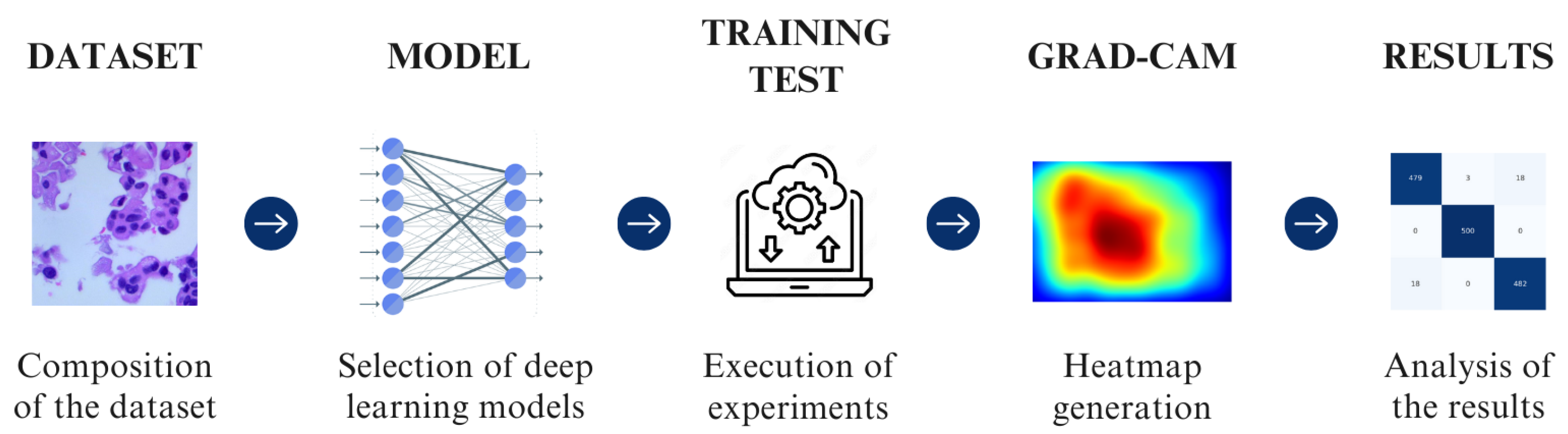
In detail, this is a multi-class classification problem because there are three classes to assign to a tissue image under analysis. Based on supervised learning, clearly all the images in the training are already labelled. As shown in Figure 1, the method adopted uses five main steps: composition of the dataset, selection of deep learning models, execution of the experiments, generation of a heatmap through Grad-CAMs, and analysis of the results.

2.1. Dataset and Preprocessing

The dataset plays a crucial role in the field of machine learning, influencing the performance, generalisation, and reliability of models. A dataset serves as the foundation for training machine learning models. The model learns patterns, features, and relationships from the examples provided in the dataset.

In the context of LC detection from tissue images, the dataset is of paramount importance for developing accurate and reliable machine learning models. Here are specific considerations for the importance of the dataset in LC detection:

• Representation of Variability: The dataset should encompass a diverse range of tissue images that accurately represent the variability in LC types, stages, and histopathological features. This ensures that the model learns to generalise well across different manifestations of LC.
• Inclusion of Normal Tissue: Alongside cancerous tissues, including samples of normal lung tissue is crucial. This helps the model distinguish between healthy and cancerous regions, promoting a more accurate diagnosis.
• Annotation Quality: High-quality annotations are essential for supervised learning in healthcare applications. The accurate labelling of cancerous and non-cancerous regions ensures that the model learns the correct patterns.
• Imbalance and Rarity: Due to the relative rarity of certain LC types or specific stages, the dataset should be carefully curated to address class imbalances. Strategies like oversampling, undersampling, or generating synthetic data can be employed to mitigate this issue.

From these aspects, it emerges that a well-curated and diverse dataset is essential for the development of accurate and clinically relevant machine learning models for LC detection from tissue images. The dataset’s characteristics directly influence the model’s ability to generalise, detect various cancer types, and contribute to the overall success of the diagnostic tool.

2.2. The CNN Models

In this paper, we exploit the following CNNs: Standard_CNN, AlexNet, VGG-16, VGG-19, and MobileNet.

In the following, a brief description of the CNNs we considered is given:

• Standard_CNN: This is a network characterised by 13 layers developed by authors. The convolutional block has three Conv2D layers based on the application of 32, 64 and 1283 × 3 size filters and ReLu activation respectively, alternating with three MaxPooling2D layers. The classification block has three Dense layers of 512, 256, respectively, with ReLu activation and three neurons with SoftMax activation, alternating with 0.5 Dropout layers, used to regularise the network. This network leverages the categorical_crossentropy loss function, as it is a multi-class classification.
• AlexNet [19]: AlexNet was the first convolutional network which used GPU to boost performance. The AlexNet architecture consists of 5 convolutional layers, 3 max-pooling layers, 2 normalisation layers, 2 fully connected layers, and 1 softmax layer. The input size is 224 × 224 × 3.
• VGG [20]: VGG-16 is a neural network architecture designed by Visual Geometry Group, the engineering sciences department of the University of Oxford. The most used versions of VGG are VGG-16 and VGG-19, which are distinguished by the number of layers. The network is inspired by the previous AlexNet but has smaller convolutional filters. The network architecture features 5 blocks of 3 × 3 convolutional layers. There are 2 convolutional layers in the first 2 blocks and 3 (in VGG-16) or 4 (in VGG-19) in the last 3. Maxpooling layers are inserted between one block and the other. Lastly, there is a block with 3 fully connected layers. The input image has dimensions of 224 × 224 × 3. We consider two different variants of this network in this paper, i.e., VGG-16 and VGG-19: the difference between these two networks is the number of layers. As a matter of fact, VGG-16 consists of 16 layers, including 13 convolutional layers and 3 fully connected layers, while the VGG-19 model has 19 layers, by including 16 convolutional layers and 3 fully connected layers. The additional layers in VGG-19 are achieved by inserting more convolutional layers in the middle of the network.
• MobileNet [21]: This network primarily uses depthwise separable convolutions in place of the standard convolutions used in earlier architectures to build lighter models. Each depthwise separable convolution layer consists of a depthwise convolution and a pointwise convolution. Counting depthwise and pointwise convolutions as separate layers, a MobileNet has 28 layers, and the size of the input image is 224 × 224 × 3.

2.3. Training

These models were inserted into the tool and trained on the dataset considered, selecting specific hyperparameters. These hyperparameters include the number of epochs, batch size and learning rate. The values that led to obtaining better results selected during the training phase are summarised in

Table 1. The table shows the hyperparameters selected during the experimentation.

Model	Epochs	Batch	Learning Rate	Ex. Time
Standard CNN	50	32	0.001	3:06:09
MobileNet	20	32	0.001	2:10:55
AlexNet	20	32	0.001	1:53:55
VGG-16	24	32	0.001	5:54:36
VGG-19	20	32	0.001	7:38:46

.

During the training phase, other experiments were carried out by changing the number of epochs, learning rate, and batch size, but they all brought lower results than those in Table 1.

In this table, we can visualise hyperparameters such as epochs, batch size, and learning rate:

• The number of epochs is a hyperparameter that defines the number of times an algorithm will work on the entire dataset. The number of epochs is usually high; this is to allow the model to learn as much as possible. You must pay close attention to the number of epochs because too high a number could lead to the onset of overfitting.
• The number of examples contained in each batch is called the batch size. In this case, selecting a batch of 32 and having a training set of 12,000 examples means to have 32 batches with 375 examples each. We will therefore have that an epoch is made up of 32 iterations. Also in this case, you must pay attention to the value selected since a batch size that is too small (<10) does not allow for performance optimisation, and if it is too large, you could have a problem of running out of memory or a greater tendency towards overfitting. Usually, the most used values are 16, 32, 64 or 128.
• This hyperparameter indicates the frequency with which the neural network updates the notions learned. Model parameters may be updated too quickly if the learning rate is too high, which may cause the model to exceed the ideal solution. Model parameters may be updated too slowly if the learning rate is too low, which may hinder convergence and require multiple training iterations to achieve the best result. Values of 0.01, 0.001 and 0.0001 are usually used.

2.4. Grad-CAM

Explainability refers to the ability to understand and interpret the decisions made by machine learning models that analyse visual data, such as images or videos. A technique exploited for explainability is the so-called Class Activation Maps (CAMs), aimed to highlight the regions of an image that are most influential in the model’s prediction. This helps users understand which parts of the input image contribute to the model’s decision for a particular class. Using architectures designed for explainability, such as interpretable deep learning models, ensures that the network’s inner workings are more transparent. These architectures are specifically crafted to provide clearer insights into the decision-making process.

In the field of CAM techniques, one of the most adopted techniques is the Grad-CAM, a technique used in the field of computer vision, particularly in the interpretation of deep neural networks, such as CNNs. It helps visualise and understand which parts of an input image were crucial in making a certain prediction by highlighting the regions that contributed the most to the final decision.

Below, there is an overview of how Grad-CAM works:

• Feedforward Pass: The input image is fed through the CNN, and the forward pass is performed to obtain the final convolutional feature maps just before the global average pooling layer.
• Compute Class Score: The class score is computed by applying the final fully connected layer to the global average pooled feature maps. This score represents the likelihood of the image belonging to a particular class.
• Compute Gradient of Class Score with Respect to Feature Maps: The gradients of the class score with respect to the feature maps are computed. These gradients highlight how much each feature map contributes to the final classification score for the predicted class.
• Global Average Pooling of Gradients: The gradients are global average pooled to obtain a weight for each feature map, representing the importance of that feature map for the predicted class. This pooling operation ensures that the importance weights have the same spatial dimensions as the original feature maps.
• Weighted Sum of Feature Maps: The weighted sum of the original feature maps is computed using the importance weights obtained from the global average pooling. This weighted sum represents the Grad-CAM heatmap.
• Rectified Linear Unit (ReLU): A ReLU operation is applied to ensure that only positive contributions are considered. This rectification helps in focusing on the regions where the class activation is positive.
• Heatmap Generation: The final Grad-CAM heatmap is obtained by overlaying the rectified weighted sum on the input image. The heatmap visually indicates which regions of the input image are crucial for the model’s decision regarding the predicted class.

By generating these heatmaps, Grad-CAM provides a visual explanation of where the CNN is focusing its attention when making predictions. This helps in understanding which parts of the input image contribute the most to the final classification decision, offering insights into the model’s decision-making process. Grad-CAM is a widely used interpretability tool in computer vision and has applications in various domains, including medical imaging and object recognition.

The primary benefits of Grad-CAM include its ability to provide insights into the decision-making process of deep neural networks, particularly in image classification tasks. This interpretability is valuable for understanding why a model made a certain prediction, especially in critical applications like medical diagnosis.

Grad-CAM has found applications in various domains, including healthcare (interpreting medical images), autonomous vehicles (understanding visual cues for decision-making), and other image-related tasks where transparency in model decisions is important.

We exploit Grad-CAM to extract the gradients of convolutional layers to produce a heatmap, a localisation map that highlights the most relevant regions of the image. These regions of the image describe which areas of the input image have most influenced the model’s output decision; in particular, the most significant areas are identified by yellow and green, and the less significant by blue.

To better understand how Grad-CAM works, in the following we provide a step-by-step mathematical implementation:

Forward Pass: Let x be the input image, $y_i$ be the predicted class score for class i, and $f_k\left(x\right)$ be the output of the last convolutional layer for feature map k.

Compute Gradients: The gradient of the predicted class score $y_c$ with respect to the feature maps $f_k\left(x\right)$ is computed using backpropagation:

$$\frac{\partial y_c}{\partial f_k}$$

This gradient reflects how much the predicted class score would change with a small change in each feature map.

Global Average Pooling (GAP): The gradients are then globally averaged to obtain a weight for each feature map:

$${\alpha }_k=\frac{1}{Z}\sum _i\sum _j\frac{\partial y_c}{\partial f_k^{ij}}$$

Here, Z is the spatial size of the feature maps, and $f_k^{ij}$ represents the activation at position $(i,j)$ in the k-th feature map.

Weighted Sum of Feature Maps: The weighted sum of the feature maps is computed to create the Class Activation Map (CAM):

$$L_{Grad-CAM}^c=ReLU\left(\sum _k{\alpha }_k{f}_k\left(x\right)\right)$$

Here, $L_{Grad-CAM}^c$ is the CAM for class c, and $ReLU$ is the rectified linear unit function.

Upsample CAM: The CAM is often upsampled to the size of the original input image for better visualisation.

Normalise and Create Heatmap: The CAM is normalised to the range [0, 1] and can be used as a heatmap:

$$H\left(x\right)=\frac{L_{Grad-CAM}^c-min\left(L_{Grad-CAM}^c\right)}{max\left(L_{Grad-CAM}^c\right)-min\left(L_{Grad-CAM}^c\right)}$$

Overlay Heatmap on the Original Image: The heatmap is then overlaid onto the original image to visualise the regions that contribute most to the predicted class.

In a nutshell, the Grad-CAM provides a way to highlight important regions in an input image based on the gradients of the predicted class score with respect to the feature maps of the last convolutional layer.

3. Experimental Analysis

In this section, we present the results we obtained from the experimental analysis of the proposed method for LC detection and localisation.

In the following section, we will present the results obtained from the experimentation. Specifically, we will analyse the metrics obtained from the classification phase, and subsequently, we will examine the Grad-CAM to understand the basis on which the model drew its conclusions.

To demonstrate the effectiveness of the proposed method, the histological image dataset (LC25000) was considered [22]. This dataset contains 25,000 colour images, of which 10,000 relate to adenocarcinomas (marked with the lung_aca label) and 15,000 relate to squamous cell lung carcinomas (marked with the lung_scc label) and benign lung tissues (marked with the lung_n label). Based on the purpose of the following study, only images relating to lung tissue were selected. To create this dataset, 750 images of lung tissue were acquired, in particular, 250 of healthy lung tissue, 250 of lung adenocarcinomas, and 250 of squamous cell carcinomas, respecting the HIPAA regulation. All images were then cropped, using a script developed by authors with the Python programming language, resulting in square dimensions of 768 × 768 pixels from the original 1024 × 768 pixels. Subsequently, the images were augmented using the Augmentor software package, which allowed an expansion of the dataset to 15,000 images, through the following augmentations: left and right rotations (up to 25 degrees, probability 1.0) and horizontal and vertical flips (probability 0.5). The dataset contains 15,000 colour images, all with a size of 768 × 768 pixels and in .jpeg file format. Following the pre-processing phase, the elements of the dataset are divided into images relating to the training set, validation set, and test set, respectively, in 80%, 10% and 10%:

-

Training Set composed of 12,000 images divided into 3 folders of 4000 images, relating to squamous cell carcinoma (lung_scc), adenocarcinoma (lung_aca), and healthy tissue (lung_n);

-

Validation Set composed of 1497 images divided into three folders of 499 elements relating to squamous cell carcinoma, adenocarcinoma, and healthy tissue;

-

Test Set composed of 1500 images of which 500 are adenocarcinoma, 500 are squamous cell carcinoma, and 500 are healthy tissue.

The experiments we conducted were carried out using the following hardware and software specifications: Intel Xeon Gold 6140 M, CPU 2.30 GHz, 64 GB RAM, with the Ubuntu 22.04.01 LTS operating system.

3.1. Quantitative Analysis

Table 2. Experimental analysis results.

Model	Accuracy	Loss	Precision	Recall	F-Measure	AUC
Standard_CNN	0.985	0.094	0.985	0.985	0.985	0.994
MobileNet	0.983	0.067	0.983	0.983	0.983	0.993
AlexNet	0.817	0.337	0.820	0.809	0.815	0.965
VGG-16	0.992	0.021	0.992	0.992	0.992	0.999
VGG-19	0.960	0.099	0.960	0.960	0.960	0.960

shows the results of the experimental analysis by showing the values obtained for the computed metrics.

To determine which model achieved better results, it is essential to ensure that the values related to accuracy, precision, recall, F-measure, and AUC are close to 1. As for the loss, its value should approach as close to 0 as possible. Taking these considerations into account and examining Table 2, it is evident that the VGG-16 model outperforms others, followed by the Standard_CNN.

The differences in performance between these models can be attributed to factors such as network depth, architecture, kernel size, and parameter efficiency. MobileNet, in particular, focuses on efficiency and is well suited for applications where computational resources are limited, while VGG-16 benefits from a balance between depth and computational complexity.

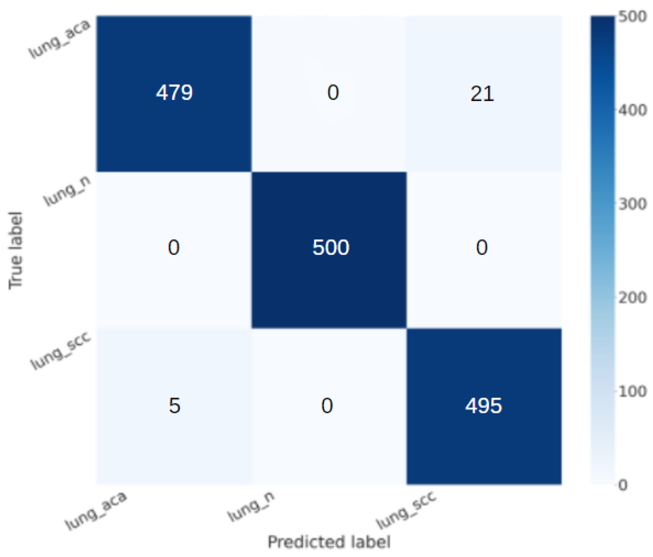
Thus, considering that the model that obtained the best performance results is the VGG-16 one, we show the confusion matrix related to this model to better understand its performance in LC detection.

A confusion matrix is a table used in machine learning and classification tasks to evaluate the performance of a classification algorithm. It provides a summary of the predicted and actual classes for a set of instances. The matrix is particularly useful when dealing with binary or multi-class classification problems.

Here are the key components of a confusion matrix:

• True Positive (TP): Instances that are actually positive and are correctly predicted as positive by the model.
• True Negative (TN): Instances that are actually negative and are correctly predicted as negative by the model.
• False Positive (FP): Instances that are actually negative but are incorrectly predicted as positive by the model (Type I error).
• False Negative (FN): Instances that are actually positive but are incorrectly predicted as negative by the model (Type II error).

Concerning the confusion matrix shown in Figure 2, the VGG-16 model shows interesting performance:

• True Positive (TP): 1000 (patients truly positive), with 500 affected by adenocarcinoma and 500 by squamous cell carcinoma;
• True Negative (TN): 500 (patients truly negative);
• False Positive (FP): 0 (patients negative but classified as positive);
• False Negative (FN): 0 (patients positive but classified as negative).

Figure 3 shows the confusion matrix related to the Standard_CNN model.

From the confusion matrix shown in Figure 3, we can note that also the Standard_CNN model is able to rightly classify most of the patients in the right category, but we note that the VGG-16 is able to obtain better performance, in fact:

• With regard to the lung_aca class, the VGG-16 model rightly classifies 491 patients, while the Standard_CNN one rightly classifies 488 patients;
• With regard to the lung_n class, the VGG-16 model rightly classifies 500 patients, while the Standard_CNN one rightly classifies 499 patients;
• With regard to the lung_scc class, the VGG-16 model rightly classifies 497 patients, while the Standard_CNN one rightly classifies 490 patients.

Comparing the confusion matrix of the remaining three models, we observe the following:

• The VGG-19 confusion matrix (in Figure 4) shows the following:

  -

  True Positive (TP): 911 (patients truly positive), with 453 affected by adenocarcinoma and 458 by squamous cell carcinoma;

  -

  True Negative (TN): 43 (patients truly negative);

  -

  False Positive (FP): 457 (patients negative but classified as positive);

  -

  False Negative (FN): 89 (patients positive but classified as negative).

• The AlexNet confusion matrix (in Figure 5) shows the following:

  -

  True Positive (TP): 987 (patients truly positive), with 487 affected by adenocarcinoma and 500 by squamous cell carcinoma;

  -

  True Negative (TN): 498 (patients truly negative);

  -

  False Positive (FP): 2 (patients negative but classified as positive);

  -

  False Negative (FN): 13 (patients positive but classified as negative).

• The MobileNet confusion matrix(in Figure 6) shows the following:

  -

  True Positive (TP): 1000 (patients truly positive), with 500 affected by adenocarcinoma and 500 by squamous cell carcinoma;

  -

  True Negative (TN): 500 (patients truly negative);

  -

  False Positive (FP): 0 (patients negative but classified as positive);

  -

  False Negative (FN): 0 (patients positive but classified as negative).

Having analysed the following results, the MobileNet confusion matrix presents a number of true positives, true negatives, false positives, and false negatives equal to those of VGG16; however, VGG16 presents higher values along the main diagonal, which allows us to consider the Standard_CNN and VGG16 better than others.

3.2. Qualitative Analysis

The Grad-CAM constitutes a valuable method for Explainable Artificial Intelligence (XAI). Explainability involves a set of tools and techniques aimed at aiding individuals in better understanding why an artificial intelligence model makes specific decisions. It addresses a common critique that machine learning and deep learning models operate as ’black boxes’, concealing their underlying functioning. The generated Grad-CAMs for Standard_CNN and VGG-16 models are presented below, utilizing heatmaps to visually highlight the most relevant areas contributing to the model’s decisions. Typically, information is encoded using colours, where significant regions are represented by colours like yellow, and less crucial areas are depicted in colours such as blue or green.

Below are the Grad-CAMs obtained from the VGG-16 model (shown in Figure 7, Figure 8 and Figure 9):

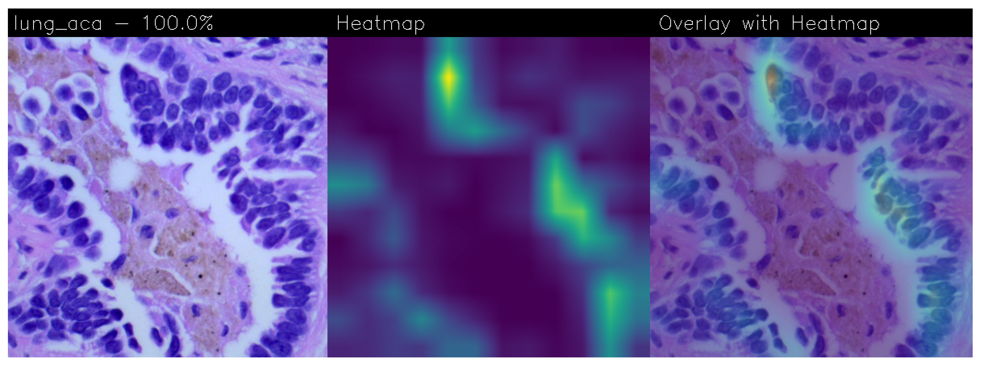
Lung adenocarcinoma is a tumour of epithelial origin that usually develops in the peripheral portion of the lung. It originates from the mucus-secreting cells that make up the mucus glands. The cuboidal and/or columnar cells of the neoplastic tissue come together to form a glandular structure. The neural network bases its decision on the geometry of the structures and the number and shape of the cells. In the central figure, the neural network recognises the most significant areas of the tumour (shown in yellow), which are actually those characterised by Pleiomorphism (increased number and size of cells), Hyperbasophilia (intensely bluish colour of the cytoplasm of the cells), and those with a higher nucleus/cytoplasm ratio (the nucleus occupies more space within the cytoplasm), which is a clear histological criterion of malignancy.

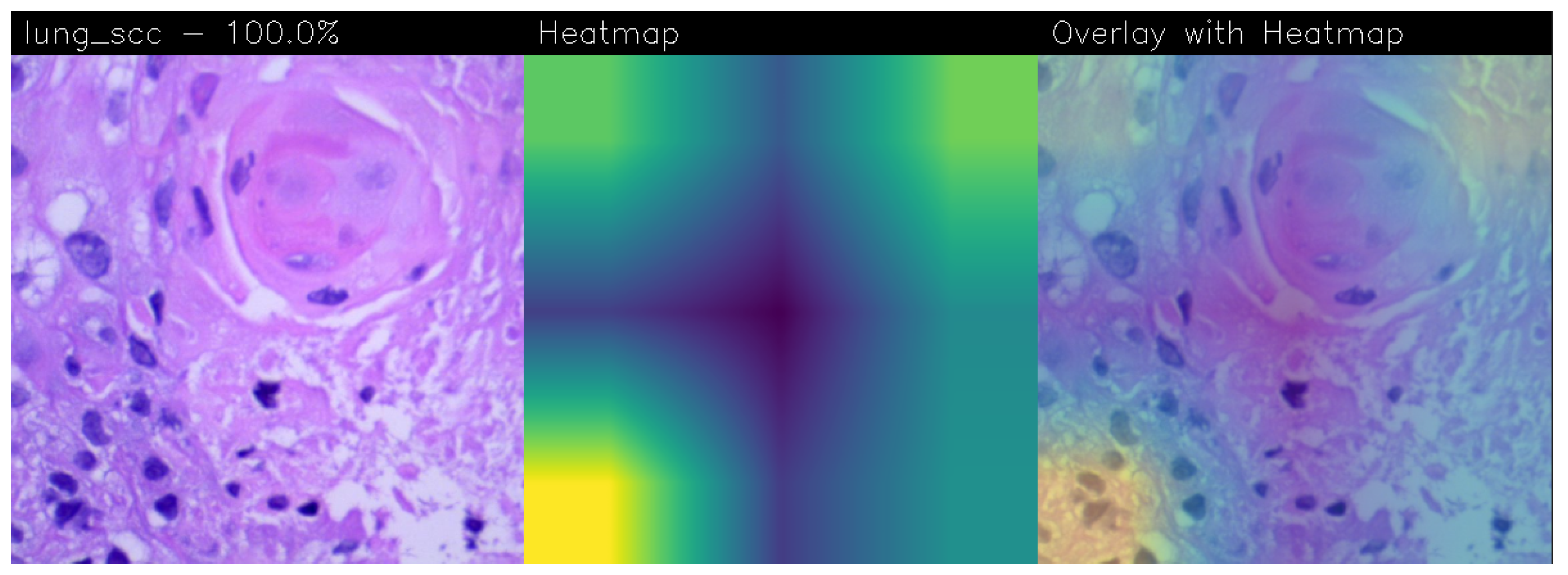
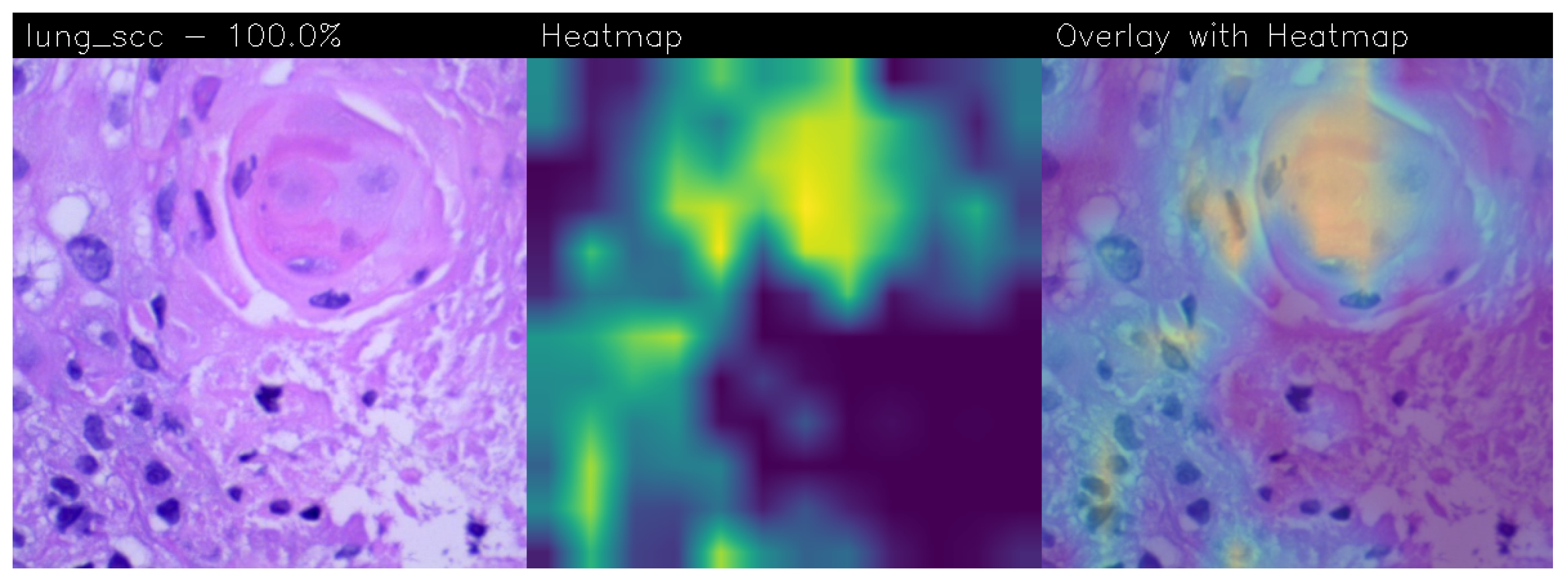
Squamous cell carcinoma originates from the squamous cells of the epithelium lining the bronchi. It is classified as such on the basis of the fish-scale appearance of the cells under the microscope, with the presence of keratinisation and intercellular bridges. From the cell membrane emerge ’spines’ that form bridges between cell and cell. The intercellular bridges are desmosomes that, together with keratinisation, demonstrate the conversion of the cylindrical bronchial epithelium into an epithelium much more similar to skin. Keratinisation is clearly visible due to the presence of eosinophilic spindle-shaped cells without nuclei. In the central figure, the neural network recognises the most significant areas of the tumour (shown in yellow) characterised precisely by an intense proliferation of cells around a point, leading to the formation of concentric areas of high keratinisation. Indeed, one of the fundamental characteristics of cancer is uncontrolled cell proliferation.

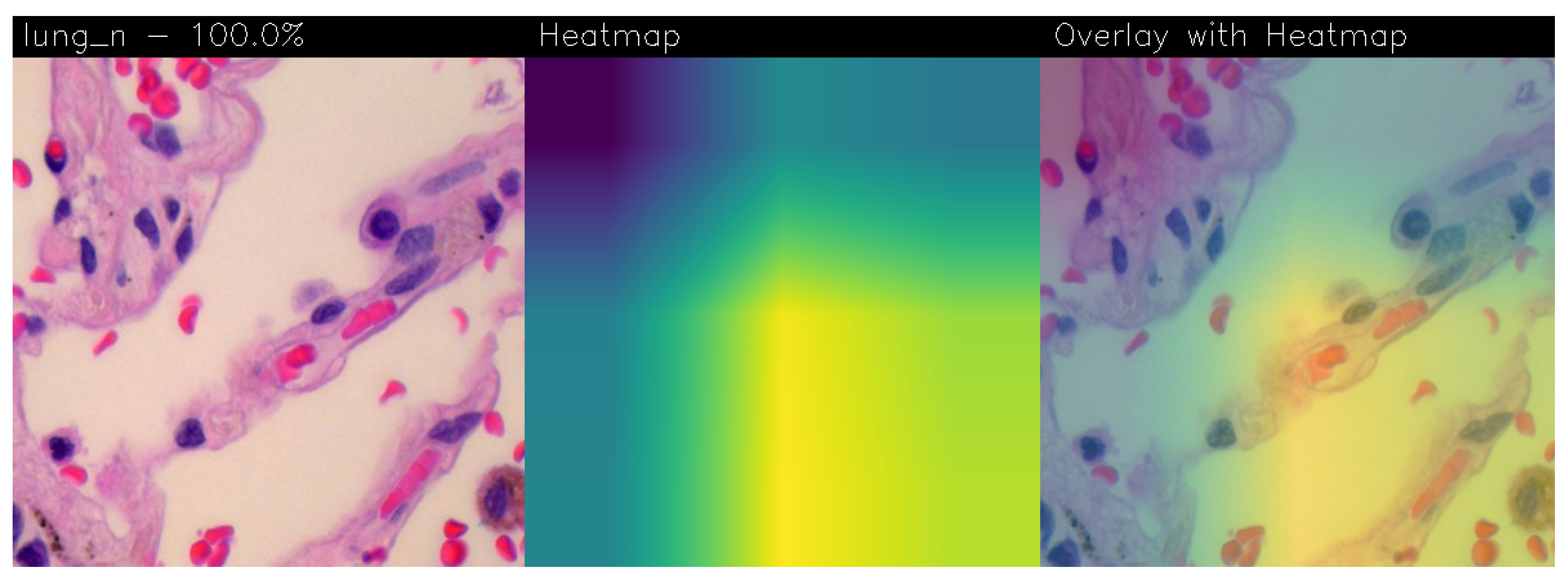
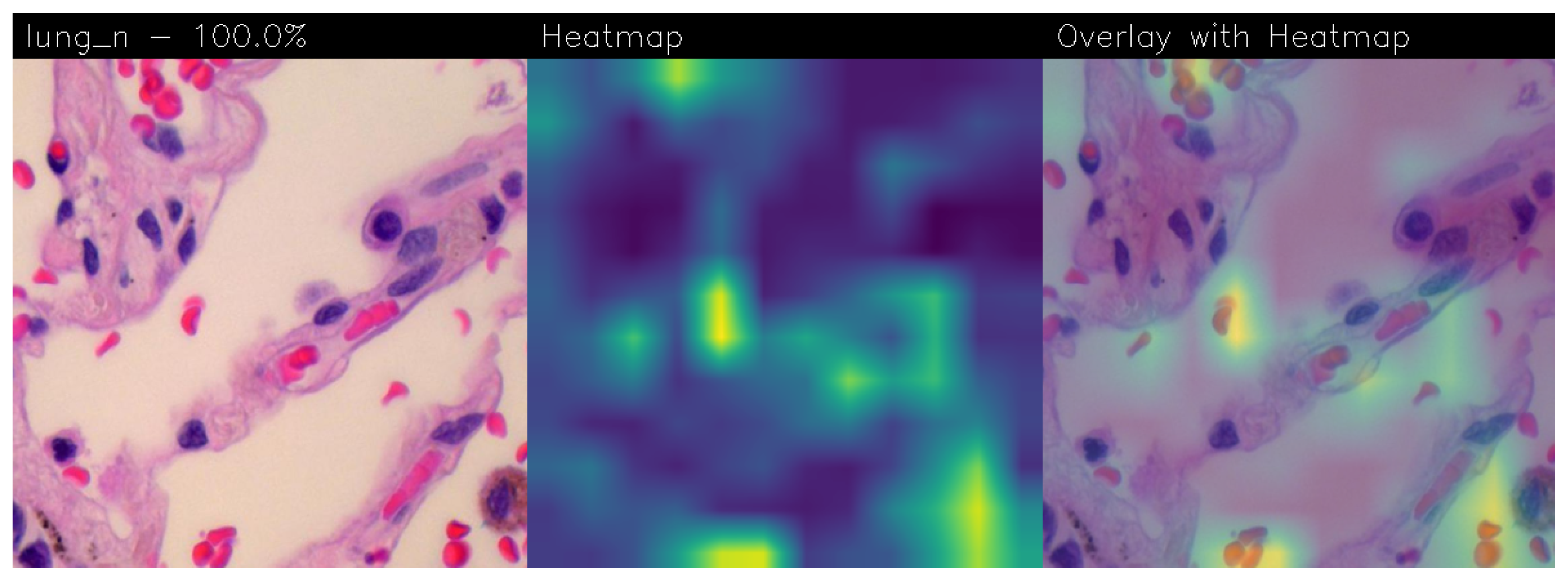
The healthy lung parenchyma consists of the pulmonary alveoli. The pulmonary alveoli are lined by a simple pavement epithelium, beneath which is the basement membrane and a thin layer of interstitial connective tissue. The epithelium consists of 95% type I pneumocytes (small cells, thin cytoplasm, and small nucleus) and type II pneumocytes (cuboidal cells and granular cytoplasm). The neural network, which bases its decision on the geometry of the structures and the number and shape of the cells, recognises the area characterised by cells with a normal nucleus/cytoplasm ratio and a normal shape and size (shown in yellow).

In the following are the Grad-CAMs obtained from the Standard_CNN model:

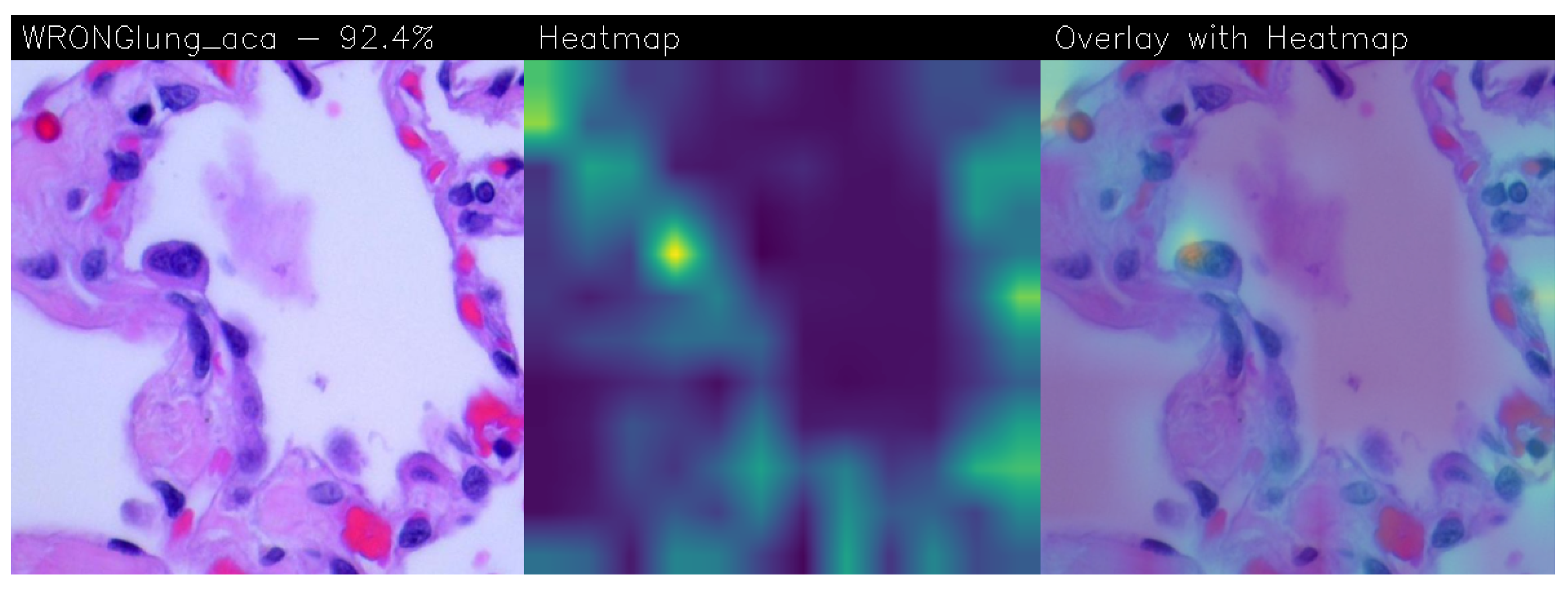
Below is presented the only false positive case, meaning the only healthy patient misclassified as diseased, identified with the Standard_CNN.

Comparing the VGG-16 and Standard_CNN models from a qualitative point of view, i.e., from the heatmaps obtained from the Grad-CAM, it is evident that the Standard_CNN tends to focus on certain areas more than others based on the presence or absence of lung carcinoma:

• In the presence of adenocarcinoma (Figure 10), the classifier relies on cells near the white portions representing mucosa or connective tissue as a distinguishing element for this class. This is because adenocarcinoma typically affects more peripheral areas, such as smaller airways like alveoli, which are surrounded by connective tissue.
• In the presence of squamous cell carcinoma (Figure 11), the classifier utilises areas with concentrations of dark or irregularly shaped cells as a distinguishing element for this class. This is explained by the fact that squamous cell carcinoma affects the squamous cells of lung tissue.
• In the case of healthy lung tissue (Figure 12), the classifier relies on red cells, specifically red blood cells, as a distinguishing element for this class.

These differentiations can be considered accurate, as lung tumours involve the uncontrolled growth of malignant cells, compromising the lungs’ function to transfer and cleanse oxygen and carbon dioxide. These functions are also related to the concentration of erythrocytes in lung tissue, as they are responsible for transporting oxygen and carbon dioxide through the hemoglobin they contain.

Therefore, a low concentration of red blood cells in lung tissue is a clear indicator of cancer.

In the case of misclassification as shown in Figure 13, the pathologist can detect it by reading the term ’WRONG’ present in the image’s top left corner. This prompts a more careful analysis of those samples as is the case for heatmaps with a low classification percentage.

With regard to the qualitative analysis of the heatmaps obtained from the application of the Grad-CAM on the VGG-16 model, the following hold:

• In the case of adenocarcinoma (as shown in Figure 10) and squamous cell carcinoma (as shown in Figure 11), the model focuses on large areas of the image, particularly near the four corners. This suggests that the model is capturing broad patterns associated with these types of LC.
• For images of healthy patients (as shown in Figure 12), the model directs more attention to one corner of the image and the centre. This may indicate that the model recognises distinctive features specific to healthy lung tissue, possibly related to the absence of irregular cell patterns seen in cancerous conditions.

Given these observations, it can be asserted that despite VGG-16 demonstrating superior overall performance, the Grad-CAMs generated using Standard_CNN appear to be more precise in identifying lung carcinoma and offer enhanced explainability. With Standard_CNN, its focus on localised patterns might contribute to its effectiveness in pinpointing specific regions associated with different lung conditions.

4. Related Work

The field in which the most progress has been made in terms of the use of artificial intelligence as a support for doctors is certainly the diagnostic one, on which there is also a series of scientific evidence present in the literature. In particular, in the oncology, respiratory, or cardiology area, thanks to the availability of images provided via X-rays, ultrasounds or CT scans, it is possible to identify, with a good degree of reliability, pathologies, both tumoural and non-tumorous, at the initial stage, even before they become important. Deep learning systems have shown their usefulness in the development of new drugs, in the analysis of radiographic images, up to the search for tumours. Deep learning allows you to analyse specific factors and cases in quantities much higher than those manageable by a human being, allowing faster decisions [23].

This section discusses the various state-of-the-art methods in lung carcinoma detection employing deep learning techniques.

One of the studies on LC classification through deep learning is that of Siddharth Bhatia et al., in which ResNet neural networks are used to detect LC from CT scans. In this study, images in DICOM format are pre-processed to extract the central region of interest of the lungs, from which features are then extracted, using deep networks inserted into classifiers for supervised learning. The results predict an accuracy of 80% [24].

Another study by Atsushi Teramoto et al. [25] proposes an automated classification scheme for lung tumours presented in microscopic images, using a deep convolutional neural network (DCNN). The evaluation results showed an accuracy of 71.1%.

Many studies also performed experiments on the same dataset used in this study, LC25000. For instance, using the LC25000 dataset, authors Mehedi Masud et al. [26] have automated the detection of colon and LC. Preprocessing of the channel-separated images included wavelet decomposition and 2D Fourier transform. They achieved an accuracy of 96.33% using a CNN model.

Neha Baranwal et al. [27] used this dataset, considering histopathological images of lung tissue, subjected to a classification into three categories: normal, adenocarcinoma and squamous cell carcinoma. This classification was carried out using ResNet 50, VGG-19, Inception-ResNet-V2, the latter being found to be better than the others with an accuracy of 99.7%, the best result among those mentioned.

Finally, the study by Daria Hlavcheva et al. [28] was based on the implementation of four different CNN models for LC classification, always using the LC25000 dataset. The input images were considered in three distinct dimensions. The maximum accuracy on the test dataset was 96.6%, using an input size of 768 × 768 pixels and a CNN model with four convolutional layers and maximum pooling layers. It was found that the accuracy increased as the size of the input image and the number of convolutional layers increased. In the study by Shankara et al. [29], a computer-aided system for detecting lung cancer using a convolution neural network (CNN) was proposed. The proposed model includes preprocessing, image segmentation model training, and tumour classification. The model was based on the Lung Image Database Consortium (LIDC), which contains 5200 lung images in which 3400 cancer lung images and 1800 non-cancer images. The proposed model classified the lung CT images as cancerous or normal image accurately with 92.96% accuracy.

In order to accurately and effectively diagnose lung cancer, the authors I. Naseer et al., presented the LungNet-SVM model for automated module identification technique in CT scans. On the LUNA16 dataset, the model demonstrated outstanding performance with 97.64% accuracy [30]. In the study by M Pradhan et al., a unique approach was constructed to automatically classify the LC25000 lung histology image collection. The accuracy rating for the EGOA (Enhanced Grasshopper Optimisation Algorithm) with random forest model was 98.50%. EffcientNetV2 big, medium, and small models are a deep learning architecture built on the concepts of compound scaling and progressive learning [31].

As shown from the comparison of the state-of-the-art literature shown in

Table 3. State-of-the-art comparison.

Reference	Year	Method	Images	XAI	Accuracy
Atsushi Teramoto et al. [25]	2017	DCNN	cytological	No	0.711
Siddharth Bhatia et al. [24]	2019	ResNet	TC	No	0.80
Neal Joshua et al. [32]	2021	3D-CNN	TC	No	0.972
Neha Baranwal et al. [27]	2021	CNN	LC2500	No	0.997
Mehedi Masud et al. [26]	2021	CNN	LC2500	No	0.963
Daria Hlavcheva et al. [28]	2021	CNN	LC2500	No	0.966
C Shankara et al. [29]	2023	CNN	TC	No	0.929
I. Naseer et al. [30]	2023	Net-SVM	TC	No	0.976
M. Pradhan et al. [31]	2023	Net-V2	LC2500	No	0.985
Our method	2023	CNN	LC2500	Yes	0.992

, to the best of the authors’ knowledge, this paper represents the first attempt considering the prediction explainability in LC detection from tissue images by exploiting CNNs. In fact, in all these studies, the explicability of the prediction in the detection of lung cancer from both CT, cytological and histological images is not considered, leading to a major limitation in considering the results reliable.

We discuss the model effectiveness for the diagnosis of cancer lung not only on the basis of quantitative results (i.e., how many pathological images they can correctly classify) but also on the basis of qualitative results, by considering the quality of explainability and on the robustness of predictions. We use an explainable deep learning method, with the aim of providing a stronger descriptive approach to the algorithm, thus improving the understanding of the data. We have not found other papers using the explainable convolutional neural networks CNN model to classify only the given three different histopathological images and the given model’s accuracy. For all these reasons, we believe that our study adds new knowledge to the already existing literature.

This research work presents lung cancer detection using histopathological images. A convolutional neural network (CNN) was implemented to classify an image of three different categories: benign, adenocarcinoma, and squamous cell carcinoma. The model was able to achieve 92% of validation accuracy. Medical professionals use histopathological images of biopsied tissue from potentially infected areas of lungs for diagnosis. Most of the time, the diagnosis regarding the types of lung cancer are error-prone and time-consuming. The main contribution of the work shows that convolutional neural networks (CNNs), one of the deep learning techniques, can identify and classify lung cancer types with greater accuracy in a shorter period, which is crucial for determining patients’ right treatment procedure and their survival rate. AI is playing a significant role in medical imaging researches. It has changed the way people process an enormous number of images.

Advances and the successful application of artificial intelligence (AI)-based diagnosis in clinical practice, especially in the field of radiology, dermatology, and pathology, is reflected with the speed of diagnosis exceeding that of experts in the medical field. Moreover, the accuracy of diagnosis through implementation of AI technologies is very high, paralleling that of medical experts [33].

The analysis of medical images, viz. X-rays, ultrasounds, MRI, computerised tomography scans and dual-energy X-ray absorptiometry, can be performed through AI algorithms. This provides assistance to healthcare professionals for the identification and diagnosis of diseases rapidly with more accuracy. The analysis of large amount of patient data can be performed by AI. These data may be related to 2D/3D imaging in the medical field, bio signals (viz., electrocardiography, electroencephalography, and electromyography), vital signs like temperature of the body, pulse rate, rate of respiration and blood pressure, information related to demography, medical history, and results of laboratory tests.

In this way, the decision-making process may be supported, and the provision of prediction results with accuracy is possible. The diversity of the data of patients in terms of multimodal data is a smart solution (optimal) that can facilitate diagnostic decisions in a better way on the basis of more than one finding, in images, signals, representation in text form, etc. Through the integration of more than one data source, the diagnosticians can gain a better understanding of the health of the patient in a comprehensive manner, and the underlying root causes in relation to the symptoms of the diseases can also be understood. The chances of misdiagnosis are also minimised in that way. Healthcare providers can be helped by multimodal data which help them in better diagnosis and the monitoring of the progress of a clinical condition over time.

This allows the therapeutic management of chronic illnesses in a more effective way. By the use of medical data (multimodal), the explainable AI (XAI)-based diagnosticians can determine potential problems of health at an early stage before the condition becomes grave and threatens the life of the patient. Further, Clinical Decision Support Systems (CDSSs) (AI-powered) provide assistance in real-time and ensure support to make informed decisions about the care of the patient in a better way. The automation of routine tasks is possible through the application of XAI tools. This frees the healthcare professionals for focusing on more complex care of patients [34,35].

Several AI-based techniques, viz. machine as well as deep learning models, are being used by researchers for detecting diseases of the heart, skin, and liver, and Alzheimer’s disease, which requires early diagnosis [36].

Machine learning has an added value for the processing of images where the identification of early signs of disease through classical tools is not possible. This is especially true for cancer, the diagnosis of which frequently requires the assistance of AI approaches [37]. It is applicable for developing nations too, where resources, cost of healthcare, and other shortcomings resist the provision of care optimally.

The Food and Drug Administration (FDA) has given a breakthrough status to AI for an algorithm (AI-based) which has the ability of diagnosing cancer in computational histopathology with tremendous precision. This facilitates pathologists with obtaining time for focusing on important slides. It is possible to develop cost-effective point-of-care diagnostics for lymphoma on the basis of basic imaging along with deep learning [38,39].

By the application of the fuzzy clustering method and neural network, successful classification and detection of people at greater risk of influenza have been performed by using rate of respiration, heart rate, and facial temperature. It is to be noted here that there is difference between fuzzy clustering methods and k-means clustering because of the addition of fuzzifier and membership values. Thus, in contrast to the non-fuzzy clustering methods, each point can belong to more than one cluster. This in turn reflects the capability of developing efficacious methods for the identification of populations at risk. In more sophisticated contexts, the application of methods of machine learning can be carried out. For example, when the support vector machine (SVM) learning algorithm, Matlab, leave-one-out cross-validation method, and nested one-versus-one SVM are used in combination, the sequences of the genes of the bacteria can be separated in a better way, thereby aiding in diagnosis more efficiently. Interestingly, there exists an artificial immune recognition system for the diagnosis of various diseases by using the properties of the immune system, such as immunological memory, which is in line with the development of AI tools on the basis of the cognitive function of humans. The artificial immune recognition system that utilises supervised methods of machine learning is found to be more accurate. Another pandemic infection that puts the life of the patient at risk is malaria. The diagnosis of malaria takes much time, and intervention of various health services may become essential. The development of machine learning algorithms has been performed for detection of red blood cells infected with the parasite from in-line holographic microscopy (digital) data, which is a relatively cost-effective technology. Various machine learning algorithms have been tried for improvement of the diagnostic capacity for malaria. The best accuracy has been shown by the model trained by SVM [40].

5. Conclusions and Future Work

In this paper, an automatic algorithm for the recognition of lung carcinoma in histological images has been proposed and developed. The developed method serves as a supportive tool for pathologists, offering a second opinion on lung biopsy diagnoses, significantly reducing analysis times, and alleviating the workload of medical professionals. This paper focuses on utilizing a deep learning algorithm, specifically, CNNs. Various CNN architectures, including MobileNet, AlexNet, VGG-19, Standard_CNN, and VGG-16, were tested. The performance results of the Standard_CNN and VGG-16 models proved to be the best, with accuracies of 98.5% and 99.2%, and AUC values of 99.4% and 99.9%, respectively. The confusion matrix analysis revealed zero misclassified patterns with VGG-16 and only one false positive with Standard_CNN, consistent with the high AUC values. These results characterise these models as highly accurate classifiers with good generalisation capabilities. The identified potentials in terms of reliability and speed could serve as an excellent foundation for future developments.

We analysed the proposed models not only from a quantitative point of view but also from a qualitative one by resorting to the Grad-CAM to have a visual explainability behind the model prediction. From the qualitative analysis, it emerged that the best model, in terms of explainability, is the Standard_CNN one. This is the reason why, considering both the quantitative and the qualitative points of view, we conclude that the Standard_CNN model is the best one for LC classification starting from tissue image analysis.

From the future work point of view, we will explore the possibility of considering other models, for instance, related to object detection, to understand whether it is possible to improve the performance obtained in terms of LC localisation. Moreover, we will investigate whether it is possible to classify other kinds of diseases related to other organs with the Standard_CNN model, for instance, by analysing tissue images related to colon tissue. In this research, a deep learning model for the localisation of lung cancer from tissue images has been proposed. In future research, artificial intelligence solutions can be leveraged for 3D lung tumour reconstruction by CT images through a novel model based on generative adversarial networks (GANs). The generative adversarial network (GAN) is a class of neural networks developed for semi-supervised and unsupervised learning. In GAN, the model learns the distribution function of the data, and then it is possible to generate new desired data by sampling it. GANs can be used to find the structure and distribution of medical imaging data and generate new images [41]. While 2D images can be valuable for many applications, 3D images provide more detail about tumour shape and geometry. Therefore, understanding the 2D/3D geometry of the tumour is necessary to show its growth behaviour and help in better surgery and drug delivery. In clinical practice, the application of AI for the purpose of diagnosis holds promise of further developments and has evolved rapidly in combination with other modern fields of tele-consultation and genomics. It is mandatory for the progress in science to remain extremely thorough and careful along with transparency for development of new solutions for improvement of healthcare in modern times. But it must not be forgotten that the focus of the health policies should be to tackle the financial issues in association with the development of various AI tools for the progress of clinical medicine. Last but not least, the experts in the medical field should understand in a better way how exactly AI should be used for the diagnosis of different diseases and illnesses. This will lead to fruitful proposals and formulating action pans in a more appropriate manner in the future for developing and exploring highly beneficial AI-based techniques in the medical field.