1. Introduction
With the development of electronic scanned array such as phased array, modern Multi-Function Radars (MFRs) are capable of performing multiple simultaneous tasks in the timeline. Moreover, MFRs can adaptively select or optimize inter- and intra-pulse modulations as well as control parameters in real time upon sensing their working environment and to meet higher-level mission demands [
1,
2,
3,
4]. The modulation patterns of each specific task feature have significant variability in control parameters such as Pulse Repetition Interval (PRI), Pulse Width (PW), and Radio Frequency (RF) [
5,
6,
7]. Accurately recognizing and analyzing the work modes of MFR is difficult and has brought urgent challenges to modern electronic receivers.
The first and preliminary step for effectively recognizing the work modes and functional intentions of an MFR is to effectively model the system. Generally, MFRs are complex systems, and their signal generation mechanism can be modeled in a hierarchical way [
6,
7,
8,
9,
10,
11]. Syntactic models are the early attempts to describe the behaviors of MFRs [
6,
8,
10]. However, first, hierarchical model-based recognition requires prior information of all the basic elements and their transition rules in each hierarchical layer, which can hardly be fully obtained in non-cooperative applications. Second, these recognition methods codify all acquired prior knowledge into an almost fixed matching template and fit intercepted signals with the context of the priors subsequently, which can hardly follow the agility in the programmable parameters of newly developed MFRs, such as a radio-defined radar or a cognitive radar [
12,
13,
14,
15]. Then, the inter pulse modulation patterns of some control parameters (namely PRI, RF, and PW) are considered as more inherent characteristics to distinguish different work modes, which provides a promising direction to explore the work intentions of MFRs [
16]. With recent advances of machine learning and deep learning, many inter-pulse modulation classification methods have been designed to deal with the recognition of modern MFRs [
16,
17,
18,
19,
20,
21,
22,
23,
24,
25,
26,
27,
28]. In the author’s previous study [
29], a sequence-to-sequence classifier is proposed to solve the pulse-level recognition problem for work modes defined as different modulation combinations of multiple control parameters. The fine-grained recognition results can further reveal the mode transition of an MFR. From these studies, a conclusion may be drawn that the supervised classification of inter-pulse modulations can be solved through deep neural networks efficiently and accurately.
However, supervised learning with pre-acquired training data constrain their potential in a realistic application for MFR signals. First, acquiring sufficient training data for numerous and programmable work modes in real complex electromagnetic environments is complicated, labor-intensive and even impossible for some special modes hidden only for emergency scenarios. Second, a deep learning classifier pre-trained through supervised learning would never be guaranteed to be efficacious under the considerations that novel adaptive sequence patterns would constantly emerge along with the development of MFR itself. An increased degree of freedom of an MFR would pose more challenges for supervised recognition methods. Last but not least, cognitive MFRs are on their way to reality [
12,
14,
15,
30,
31], which could work in a more fine-grained mode with the same modulation but different parameters to meet different performance requirements. It is of great importance to investigate recognition methods that require less prior information.
Generally, intercepted radar pulse sequences are represented using Pulse Descriptor Word (PDW) sequences. In terms of unsupervised learning, Guan [
32] employs the concept of the Needleman-Wunsch algorithm and utilizes sequence alignment processing to obtain the MFR search mode rules. Fang [
33] proposed an unsupervised change-point detection algorithm based on the Bayes criterion to recognize MFR work modes. Liu [
34] proposed a semantic encoding model and encoding strategy optimization method for MFR pulse sequences. This method can automatically discover sequence patterns of MFR pulse sequence signals and represent them in the simplest form for extraction. However, these methods are applicable to a limited range of MFR work modes. Further research is needed to adapt them to new radar systems with modulation such as agile modulation. Taking the PDW sequences as Multivariate Time Series (MTS), unsupervised feature extraction and clustering methods can be investigated for a more general applied and less prior required solution. There are recent studies considering the time series clustering of radar signals [
22,
35]. Guillaume [
35] focus on clustering pulse sequences from different radar emitters, and the mean value is used to represent the time series characteristics of a pulse sequence. Their method achieves satisfactory performance as the parameter values of different emitters are differentiable in high-dimensional PDW spaces. However, for an MFR, the parameter values of different work modes are close or even overlap; these methods would suffer performance degradation. In [
22], parametric models for different PRI modulations are established, and three clustering methods are proposed for sub-sequence clustering of MFR work modes. However, clustering of multivariate time series requires further investigation. In fact, the clustering of multivariate time series has been investigated in many other fields. There are many comprehensive reviews for time series clustering [
36,
37,
38,
39,
40] and a variety of investigations of multi-variate time series feature extraction or clustering methods [
41,
42,
43,
44,
45,
46,
47,
48,
49]. However, to the best of our knowledge, there is still a lack of investigations into the recognition of MFR pulse sequences from a multivariate time series clustering perspective.
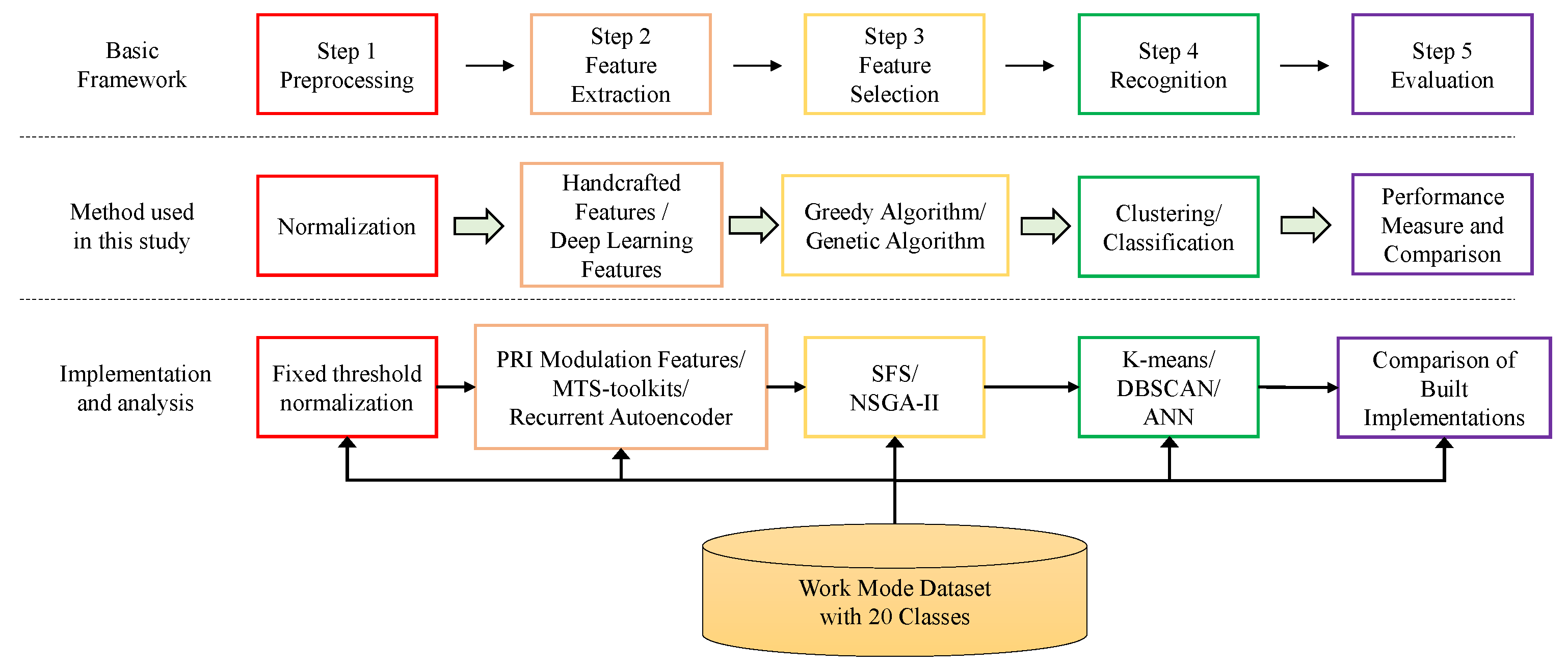
This paper puts its focus on establishing a multivariate time series feature extraction and clustering framework for MFR pulse sequences and selecting the optimal features for MFR work mode recognition. The clustering framework consists of five steps: pre-processing, feature extraction, feature selection, recognition, and evaluation. In the feature extraction part, manual feature and deep learning feature extraction methods are separately studied, including (1) feature engineering from hand-craft features for PRI modulation-type identification, (2) feature engineering from extensively designed MTS hand-craft features, and (3) unsupervised automatic feature engineering with deep neural networks. Extensive experiments are conducted to verify the effectiveness of the proposed clustering framework. Experimental results validate the superiority of the proposed framework and the effectiveness of the selected features. The main contributions of this paper can be summarized as follows:
- (1)
A multivariate time series feature extraction and clustering framework is designed for MFR pulse sequences.
- (2)
Several different implementations of the proposed framework are evaluated and compared. In each implementation, effective and advanced methods are utilized.
- (3)
The experimental dataset includes a rich variety of radar modulation patterns; therefore, the selected features possess better universality.
The rest of this paper is organized as follows.
Section 2 describes the formulation of the feature extraction and clustering tasks for multivariate MFR time series.
Section 3 introduces the proposed framework and the corresponding implementations. Data description, experimental design, and experimental results are provided in
Section 4. Finally, the conclusions and guidelines for future work are provided in
Section 5.
2. Problem Formulation
This paper aims to implement a multivariate time series clustering framework for MFR pulse sequences. This section describes the definition of MFR work modes, provides definitions of work mode sequences, and presents mathematical formulation of the recognition task.
2.1. MFR Work Modes Definition
To serve multiple radar functions, each MFR work mode class has different intra- or inter-pulse parameters and can be defined as a certain arrangement of a finite or variable number of pulses. The author’s previous study [
29] defined the time series representation of an MFR work mode sequences which are briefly introduced here for completeness.
At first, an MFR work mode can be defined as modulation combinations on multiple control parameters [
7,
11,
29,
50], more specifically, in this study, the PRI, RF, and PW. Then, two layers of work modes can be derived to described the ability of MFR and CR to adaptively select or optimize modulations or modulation parameters. The modulation-level work mode represents the fact that the MFR can select or optimize modulations or modulation parameters in corresponding modulation and parameter space. The final optimized result is denoted as parameter-level work mode and it can be seen as an implementation or instantiation of the modulation-level work mode. An input MTS with
n pulses of the corresponding MFR work mode can be described as
, where
M is the number of parameters and each parameter in the pulse sequence obeys certain time series characteristics according to the modulation types.
There are different inter-pulse modulation styles for the three selected parameters. Six classes of modulation are employed in this study, including constant, agile, jittered, dwell and switch, sliding, and periodic. The candidate modulation types corresponding to the three parameters are listed in
Table 1.
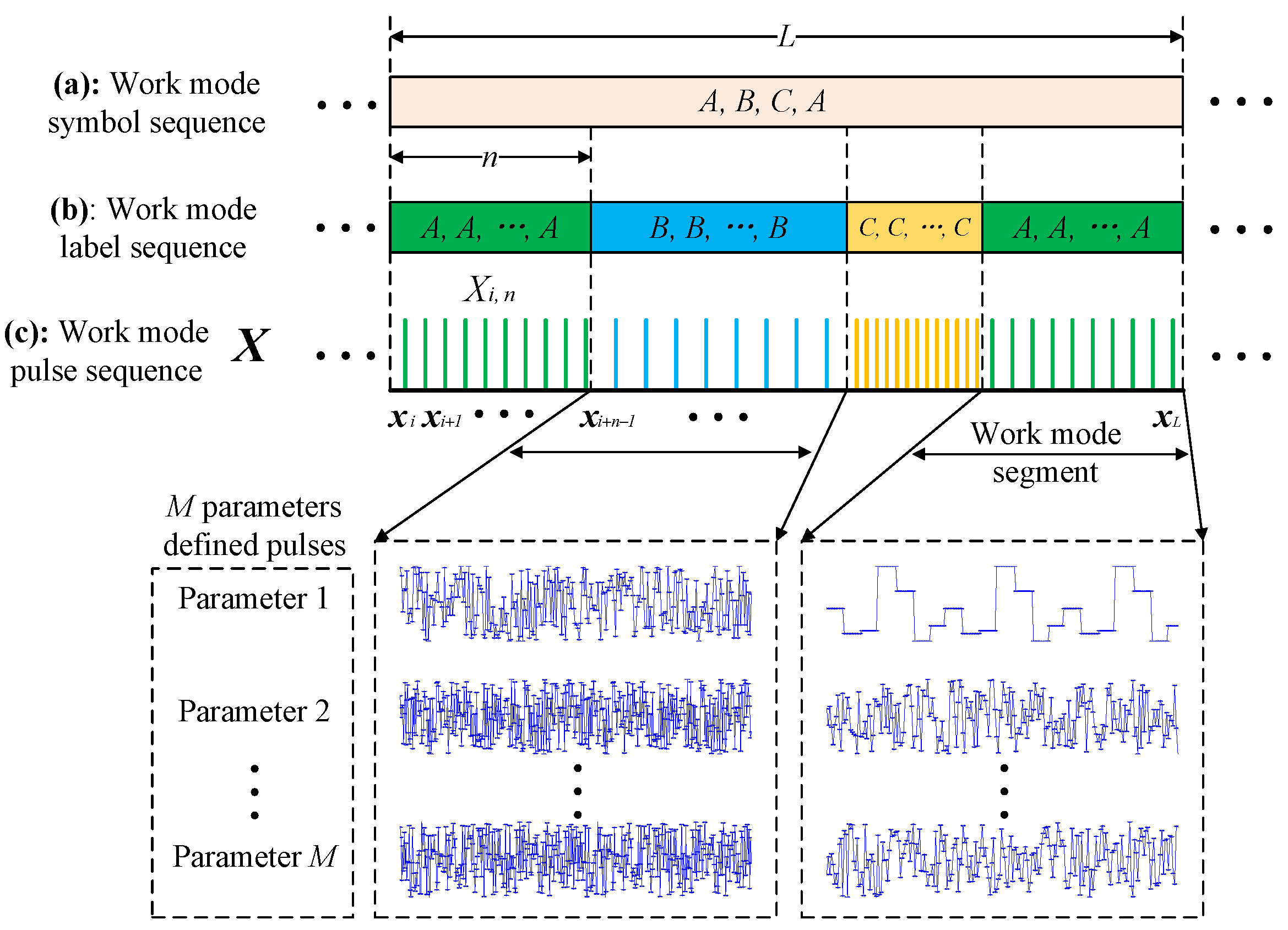
2.2. Time Series Representation of an MFR Pulse Sequence
An MFR work mode sequence can be defined in a multiple-layer architecture, as described in [
29].
Figure 1 illustrates the
M parameters defining an MFR work mode sequence.
Definition 1. A radar pulse is represented by a real-valued vector of M parameters as .
Definition 2. A of L pulses is a of ordered pulses .
Definition 3. A of n pulses in is a sub-sequence of pulses , where . Each belongs to a certain class, while different may belong to the same class.
Definition 4. A of J work mode segments and K work mode classes is a data structure that stores the work mode class symbols. A symbol represents the work mode class of a in . For instance, an with as ‘A, B, C, A’ contains four consecutive from three classes.
Generally, the investigation of both feature extraction and clustering methods should utilize the radar segments from the individual work mode. Through such operation, the effectiveness of the extracted features and the performance of the clustering methods can be evaluated and compared with specific physical meanings. In applications, the input radar pulse sequence generally contains multiple segments from different work mode classes. In such a case, the investigated feature extraction and clustering methods can be combined with sliding window techniques [
16] for sub-sequence clustering [
39] of pulse sequences with multiple work modes; this is another area of discussion. To keep this paper well focused, in the following sections, all methods are investigated in samples with a single work mode class.
2.3. Multivariate Time Series Clustering Task of MFR Pulse Sequences
An MFR pulse sequence clustering task is expected to output a cluster label for each input work mode sample. We let denote the MFR pulse sequence dataset with N pulse sequence samples. An input sample consisting of L pulses can be expressed as , 1 , where , is the tth pulse, and M is the number of pulse parameters. The goal for the clustering task is to compute cluster labels for based on the similarity of the samples.
Generally, direct calculations of the similarity between are complicated due to great variability in number of pulses for different samples. Although dynamic time warping is a useful tool for similarity measuring of sequences with unequal length, its computational complexity is high for longer sequences. In this paper, the input pulse sequences with variable length are at first transformed to the feature space through function , where is the extracted feature vector set. The clustering task is to divide feature dataset into K clusters by measuring the similarity in the feature space.
3. Methodology
Based on existing investigations on multivariate time series clustering, in this paper, a framework of feature extraction and unsupervised clustering is designed. This section at first describes the overall framework for MTS work mode clustering and then separately introduces the details of each step.
3.1. Framework Architecture
As shown in
Figure 2, the general framework contains five steps including preprocessing, feature extraction, feature selection, recognition, and performance evaluation. In the feature extraction step, three sets of features are collectively extracted to form the entire feature set. Based on different method configurations in feature selection and recognition steps, different implementations are considered suitable for an MFR work mode pulse sequence.
3.2. Preprocessing Method
Since a pulse is usually represented by multiple parameters (i.e., M in this paper) which have different units and orders of magnitude, normalization is often necessary to bring all parameters to a comparable scale. A common normalization approach involves scaling parameter vector based on its maximum and minimum values.
In the context of work mode recognition, a sequence may not encompass all work mode classes. Consequently, if normalization is solely based on the existing classes in the sequence, the relative relationships between each class may be disturbed, leading to recognition errors. This impact becomes more pronounced during the testing phase, as received testing sequences are not guaranteed to contain all mode classes within a given time duration.
Hence, in this paper, pulse sequences are normalized based on fixed lower and upper bounds
and
for the
M parameters, utilizing the following formula:
where
represents the mth parameter vector of the input sequence and is normalized by the corresponding lower and upper bounds
and
. The values of
and
can adhere to the statistical range of pulse parameters. Therefore, normalizing with absent classes helps avoid issues of disrupting relationships.
3.3. Feature Extraction Methods
The sequence dataset with N samples is transformed to feature matrix ; n is the number of extracted features.
3.3.1. PRI Modulation Features
An efficient feature set for pulse repetition intervals modulation recognition (PRI Modulation Features) is proposed by researchers in [
16]. The feature set includes several histograms and sequential features of PRI to describe specific modulation types. By cascading simple multilayer neural networks for classification, excellent modulation type recognition results can be achieved. In this study, PRI modulation features are extended to accommodate the condition of three parameters and the clustering task.
3.3.2. MTS Features
We represent the radar work mode PDW sequence as an MTS. Therefore, we seek effective multivariate time series features for radar mode recognition. For example, in 2020, researchers in Georgia state university [
51] presented a python toolkit for feature extraction of MTS which includes a comprehensive set of statistical features for extracting the important characteristics of MTS. In this paper, 39 kinds of these statistical features for each variate are extracted and added to the pool of candidate features.
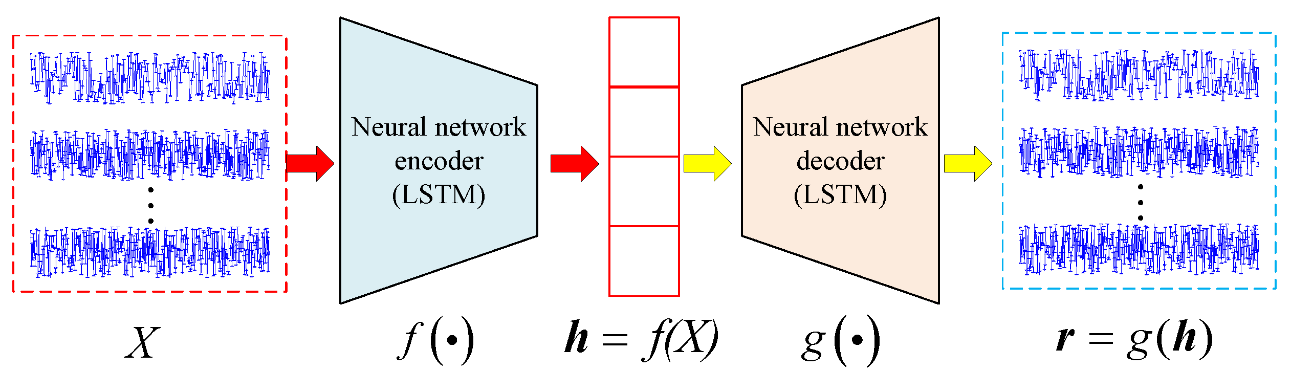
3.3.3. Unsupervised Neural Network Features
With the development of artificial intelligence and deep learning, automatic feature extraction become prevalent in pattern recognition. Autoencoders (AEs) are mature yet effective unsupervised feature extraction methods. For AEs, the encoder function at first encodes
X to hidden representation
, then the decode function
decodes
to reconstruct
X. There are reconstruction errors between
and
X. The goal for an AE is to minimize the reconstruction error,
. Generally,
and
are non-linear mappings, and thus AE is considered to extract more general and robust features. Since the raw MFR pulse sequences are with variable length and are multivariate time series, Recurrent AE (RAE) is utilized to extract time series features. The main difference between RAE and AE is that the encoder and decoder of RAE are Long Short-Term Memory (LSTM) layers, while for AE they are fully connected layers. LSTM layers are inherently suitable for extraction of time series features from raw time series data [
52,
53]. The structure of RAE in this paper is shown in
Figure 3.
We let
denote the MFR pulse sequence dataset with
N pulse sequence samples. An input sample consisting of
L pulses, which can be expressed as
,
. The goal for the RAE is to compute
for
based on
and
. The RAE is trained to minimize reconstruction errors
in the training dataset. The loss function is expressed as follows:
After the RAEs are trained, the output of encoder function when receiving testing pulse sequence X is treated as the extracted features.
3.4. Feature Selection Methods
The feature selection process is formulated as a multi-objective optimization (MOO) problem with selecting fewer MTS features and higher clustering performance as two optimizing objectives. The first objective function is
, where
denotes the performance evaluation metrics of the clustering results for a given feature combination. The second objective function is the total number of the selected variables,
. Thus, the MOO problem can be formulated as follows:
Wherein decision vector
is used to formulate the identification of important features, where
The decision vector controls the selection of the subset of features for evaluation. Two methods are utilized and compared to solve the MOO problem for feature selection. The greedy search algorithm based on sequential forward selection and the heuristics method based on the Non-dominated Sorting Genetic Algorithm.
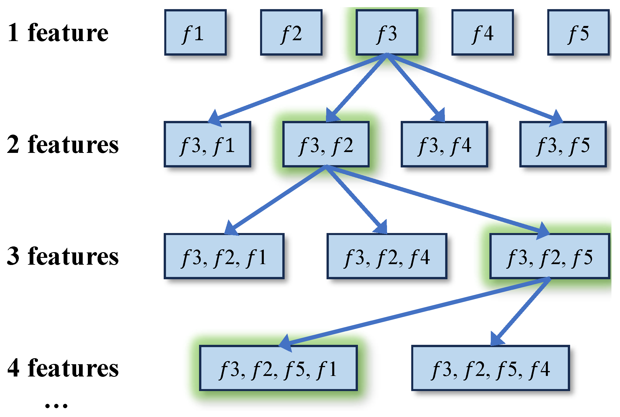
3.4.1. Sequential Forward Selection (SFS)
Sequential forward selection is a greedy algorithm with fast solution speed and low time complexity. In the SFS, feature subset
F starts from the empty set and adds one current optimal feature
f to
F each time to make the feature selection
the local optimal. The general process of SFS implementation is shown in
Figure 4, Algorithm 1.
| Algorithm 1 Sequential Forward Selection (SFS) |
1: Input complete feature set Y, maximum number of feature subsets K
2: Initially the feature subset F to an empty set.
3: In each iteration, select feature f from the complete feature set Y and add it to F such that the feature evaluation function achieves the maximum value.
4: Check whether the current number of features k is equal to the desired number of feature subsets K.
5: If yes, stop; otherwise, repeat the previous step until the condition is satisfied.
|
3.4.2. Non-Dominated Sorting Genetic Algorithm (NSGA-II)
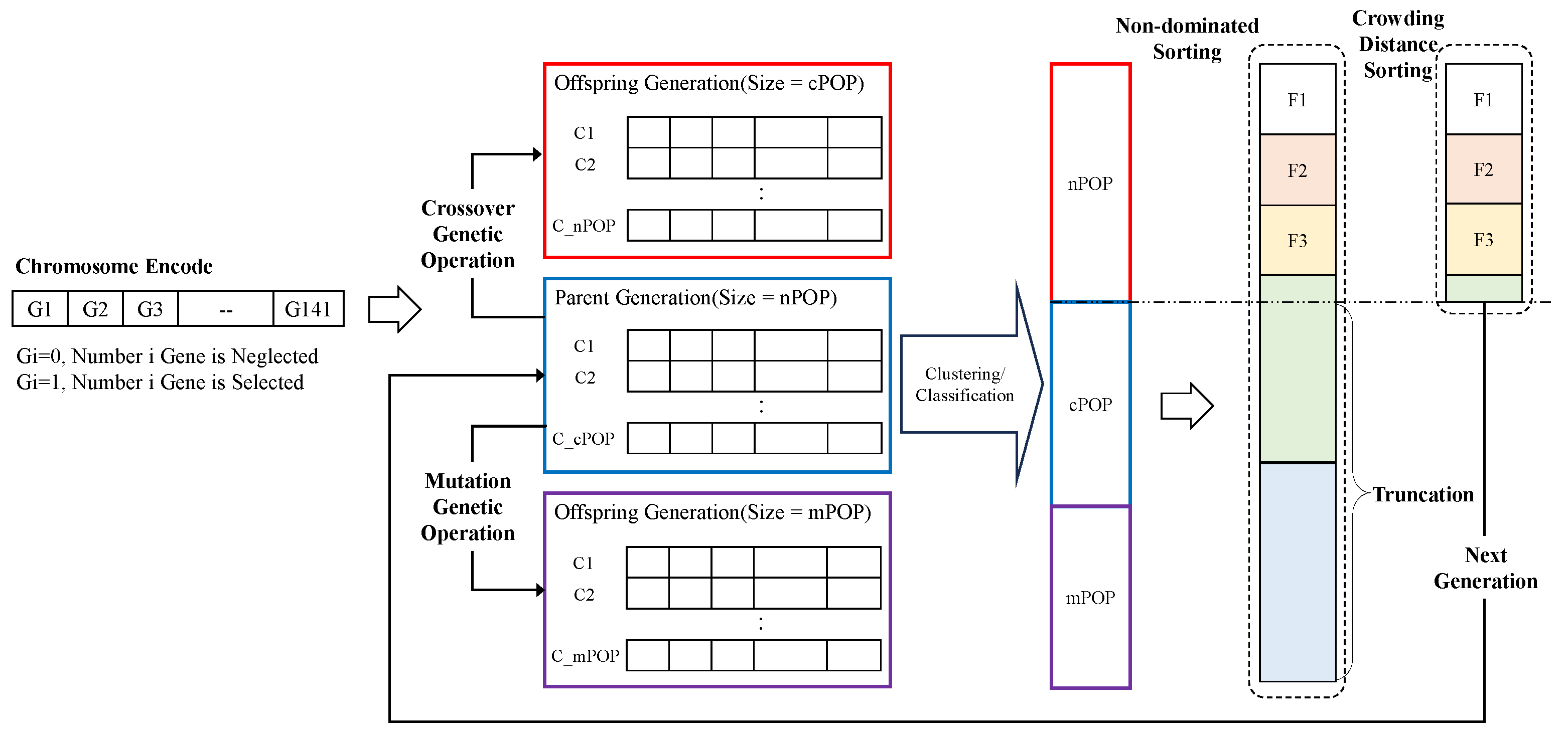
A genetic algorithm is a heuristics search method for solving MO problems. The non-dominated sorting-based multi-objective evolutionary algorithm (NSGA-II) [
54,
55] is utilized in this study. NSGA-II adapts a suitable automatic mechanism based on the crowding distance (CD) to guarantee the diversity and spread of its solutions. The NSGA-II chromosome is encoded in a 141-bit binary sequence. Each bit represents a corresponding feature, and the whole string represents some combination of the candidate feature set. For population initialization, parents with nPOP chromosome sizes are randomly generated. In each subsequent cycle, through genetic operators of crossover and mutation, two offspring populations are generated from the corresponding parent. The sizes of the two offspring populations are cPOP and mPOP, respectively. For each individual in the simulated population, all “1” bit fields in the chromosome will be retrieved from the original feature set and connected to the clustering or classification input. Then based on the output of two objective functions, better qualified chromosomes are chosen through the NSGA-II algorithm. At the end of the simulation of the iterations, the algorithm converges to the best chromosomes that represent the optimal or sub-optimal solutions. The general process of NSGA-II implementation is shown in
Figure 5, Algorithm 2.
| Algorithm 2 Non-dominated Sorting Genetic Algorithm (NSGA-II) |
1: Input complete feature set Y, maximum number of iteration limit L
2: Initially, randomly select a subset of features from the original feature set as the first-generation population P.
3: In each iteration, select excellent individuals by sequentially comparing the labels and Crowding Distance (CD) values of two individuals.
4: Apply crossover and mutation operations to generate a new generation population Q.
5: Merge P and Q into a combined population R, and similarly use two levels of preference operators to select the optimal N individuals from R as the next-generation population.
6: Check whether the preset iteration limit L is reached.
7: If yes, stop; otherwise, repeat the previous step until the condition is satisfied
|
3.5. Recognition Methods
Although our proposed framework primarily operates through unsupervised clustering methods for MFR work mode recognition, supervised classification methods are also included in the recognition process to validate the effectiveness of the selected features. There are already many mature yet effective clustering methods including distance-based, density-based, and spectral based ones [
56]. In this study, one distance-based clustering method (K-means) and one density-based clustering algorithm (Density-Based Spatial Clustering of Applications with Noise, DBSCAN) are employed in the clustering step. K-means models are widely used in radar signal sorting [
57] or clustering of different radar emitters [
58]. DBSCAN is a density-based spatial clustering of applications with a noise algorithm [
59] which does not require the priors of the number of clusters. During clustering, various distance metrics such as Euclidean distance and Cityblock distance are experimented with. In the end, Euclidean distance is selected for the experiments. Simultaneously, artificial neural networks are employed as a classification method to validate the effectiveness of the features.
4. Experiment and Analysis
In order to verify the effectiveness and superiority of the proposed framework and selected features, experiments with simulated MFR work mode pulse sequences were conducted. The experimental design, the datasets, and the evaluation metrics are described in
Section 4.1. Then, the experimental results and the discussions are presented in
Section 4.2,
Section 4.3 and
Section 4.4.
4.1. Experimental Design
4.1.1. Dataset Description
According to
Section 2.1, 20 classes of MFR work modes are considered (i.e.,
) based on different combinations of inter-pulse modulations on Pulse Repetition Interval (PRI), Radio Frequency (RF), and Pulse Width (PW), as depicted in
Table 1.
Table 2 shows the corresponding value ranges of modulation parameters for PRI, RF, and PW, respectively. Three kinds of non-ideal conditions including measuring noise, lost pulse, and spurious pulse are considered in the experiments. The three basic non-ideal settings are Measuring Noise Only (MNO), Lost Pulse Only (LPO), and Spurious Pulse Only (SPO). The MNO adds Gaussian distributed measuring noises to PRI, RF, and PW, respectively. The Gaussian noises have zero means and standard deviations in common units as
. There are seven levels of measuring noises according to variations of
as
,
. For instance, the first level is
, and the second level is
. Both LPO and SPO separately consider the pulse sequences with a proportion of lost or spurious pulses. There are seven levels for both lost pulse and spurious pulse proportions with a range of [0:5:30]%. In addition, seven hybrid scenes are defined to evaluate the joint influence of combined non-ideal situations as depicted in
Table 3. Thus, there are seven datasets for MNO, LPO, SPL, and hybrid scenarios, respectively. For each work mode class in each dataset, 500 samples are simulated, and there are a total of 10,000 sequence samples for each dataset. The number of pulses in a work mode sample is set to 200. In addition to simulated data, we also collected some actual measured signals to form the measured scenarios.
4.1.2. Evaluation Metrics
Clustering purity and Normalized mutual information (NMI) are two fundamental evaluation metrics for assessing clustering performance, while cross-entropy loss serves as a fundamental metric for evaluating multi-class classification performance. This study employs these three metrics for performance evaluation. The descriptions of these three metrics are as follows:
The clustering purity is defined as
where
N is the total number of samples.
denotes the clustering results.
denotes the real assignments.
- (2)
Normalized mutual information
Normalized mutual information can be described as
where
is mutual information and
is entropy. They are defined as [
60]
where
and
denote the possibility of a sample belonging to cluster
, category
, and both of them, respectively.
represents the increase in cluster information
for given class information
C. That is,
- (3)
Cross-entropy loss
Cross-entropy loss is a commonly used loss function in machine learning and particularly in the context of classification problems. It measures the performance of a classification model whose output is a probability value between 0 and 1. The goal of the model is to assign the correct label to each input. For a multi-class classification problem with
K classes, the formula is a generalization:
where
is the indicator function that equals 1 if the true class is
i and 0 otherwise,
is the predicted probability that the instance belongs to class
i.
4.1.3. Experimental Design
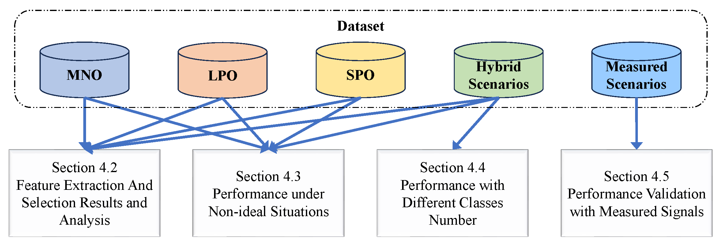
Combining two different feature selection methods with three different recognition methods results in a total of six implementations. Therefore, experiments were conducted using each of these implementations individually as follows (
Figure 6):
- (1)
Feature selection results analysis for different optimization methods (
Section 4.2).
- (2)
Robustness against typical non-ideal situations (
Section 4.3).
- (3)
Performance against different numbers of MFR work mode classes (
Section 4.4).
- (4)
Performance validation with measured signals (
Section 4.5).
4.2. Feature Extraction and Selection Results and Analysis
In order to make the selected features more universally applicable, during the feature selection process, the dataset is formed using data from all 20 classes of working modes in all non-ideal condition scenario datasets. For each class of data in each scenario dataset, 50 random samples are selected and added to the complete dataset
. Feature extraction is then performed on the dataset using the three feature extraction methods described in
Section 3.3, resulting in a complete feature set
Y.
Figure 7 presents the t-Distributed Stochastic Neighbor Embedding (t-SNE) visualization results of all feature sets. From this, it can be observed that, before feature selection, different work mode classes are challenging to distinguish, indicating the presence of redundant features within the feature set.
Based on six implementations composed of different feature selection and clustering methods, features of the MFR work mode are selected, and the results are depicted in the figure. The optimization objectives and maximum iteration count for each implementation are shown in the table below (
Table 4).
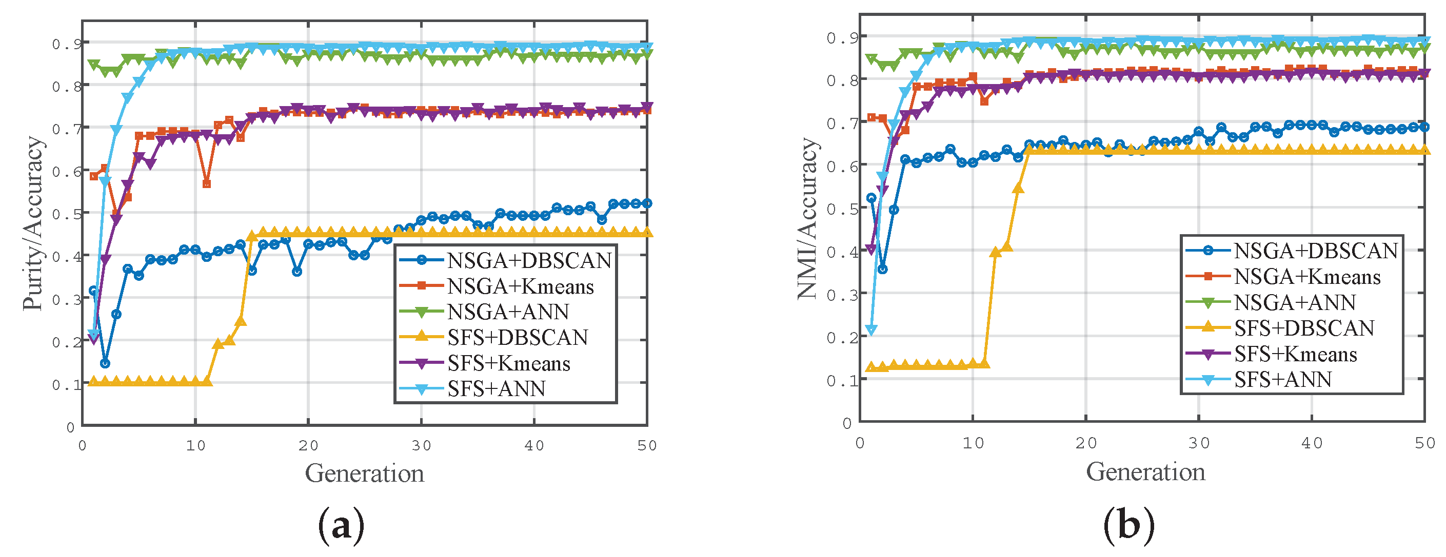
Figure 8 illustrates the performance changes during the iterative process of feature selection for different implementations. It can be observed that the iteration performance of the NSGA-II algorithm is superior to that of the SFS algorithm. This is because NSGA-II possesses strong global search capabilities, allowing for it to find widely distributed solutions in the search space. In contrast, SFS is prone to becoming stuck in local optima, especially when the clustering method is DBSCAN, quickly converging to a local optimum without further optimization. Additionally, since the K-means clustering method has a known number of clusters and strong prior information, its performance is better than that of the DBSCAN clustering method. As a supervised classification method, ANN exhibits the best performance and quickly reaches convergence. This demonstrates that the selected features have clear discriminability in a high-dimensional space.
Table 5 presents the distribution of the selected number of features for each implementation. It can be observed that the proportion of PRI modulation features is relatively high, indicating that features designed specifically for radar parameter inter-pulse modulation types are more effective. The relatively small proportion of MTS features is due to the fact that some features in this MTS feature extraction toolkit are only suitable for continuous time series, while PDW sequences are discrete and not suitable for these features. Finally, there is considerable room for improvement in features based on deep learning. In the future, network structures can be improved and regularization terms can be added to extract more effective features.
4.3. Performance under Non-Ideal Situations
The pulse stream is often contaminated by highly non-ideal electromagnetic environments. A good method should be robust enough to correctly identify corrupted pulse sequences. This section evaluates the performance of different methods under non-ideal conditions, including three distinct non-ideal scenarios: MNO, LPO, SPL, and hybrid scenarios.
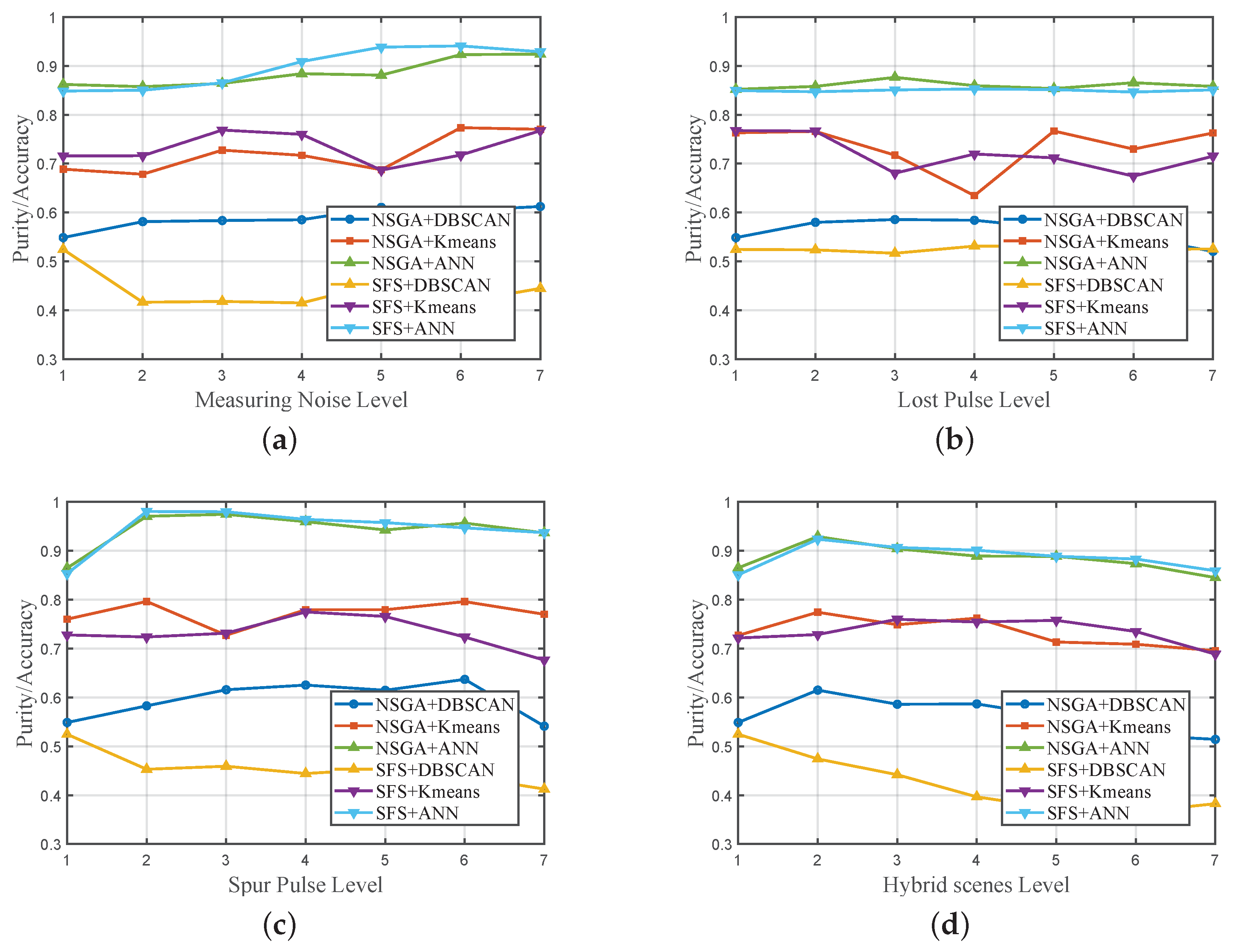
The clustering purity/classification accuracy for each implementation in different scenarios is displayed in
Figure 9, separately. Due to the supervised nature of the ANN method, which involves utilizing more prior information, the classification accuracy is significantly higher than the clustering purity of other clustering methods. Different feature selection methods have little influence on the ANN method, and the classification accuracy remains above 84% in all scenarios.
In the MNO scenario, noise does not cause substantial negative effects on all implementations. In fact, there is even some performance improvement in measuring more severe noise conditions. The reason may be that when the noise is relatively low, the impact of different parameters of the same working mode is too significant, leading to a relatively large intra-class distance. As the noise increases, the intra-class distance becomes relatively smaller, making it easier to distinguish between different classes.
In the LPO scenario, each implementation can maintain stable performance, with relatively minor effects from changes in the proportion of missing pulses. The K-means clustering method, due to its sensitivity to the initialization of clustering, exhibits slightly larger performance fluctuations. The selected features and clustering implementations demonstrate good robustness to the situation of missing pulses.
For the SPL scenario and the hybrid scenario, the diversity introduced by spurious pulses increases the variability of sample features. Therefore, under non-ideal conditions, there are instances where performance may show some improvement. However, the overall performance in the mixed scenario tends to decrease as non-ideal conditions worsen.
In summary, the proposed implementations and the selected features exhibit good robustness in non-ideal scenarios, providing satisfactory distinctiveness in both unsupervised clustering and supervised classification. Among clustering implementations, NSGA+Kmeans performs better than others.
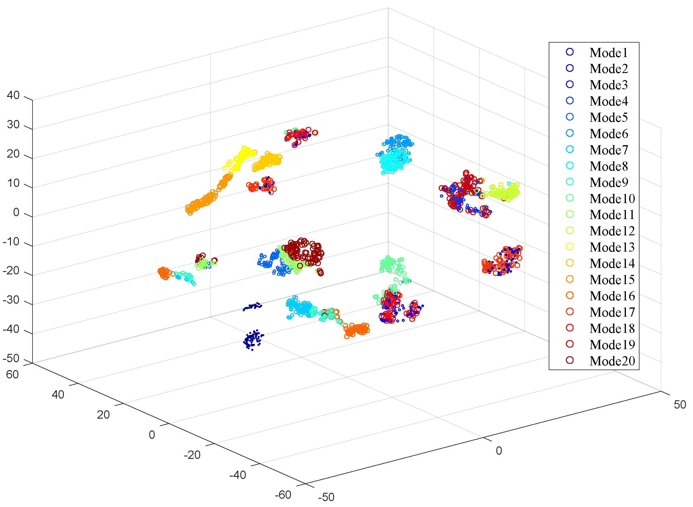
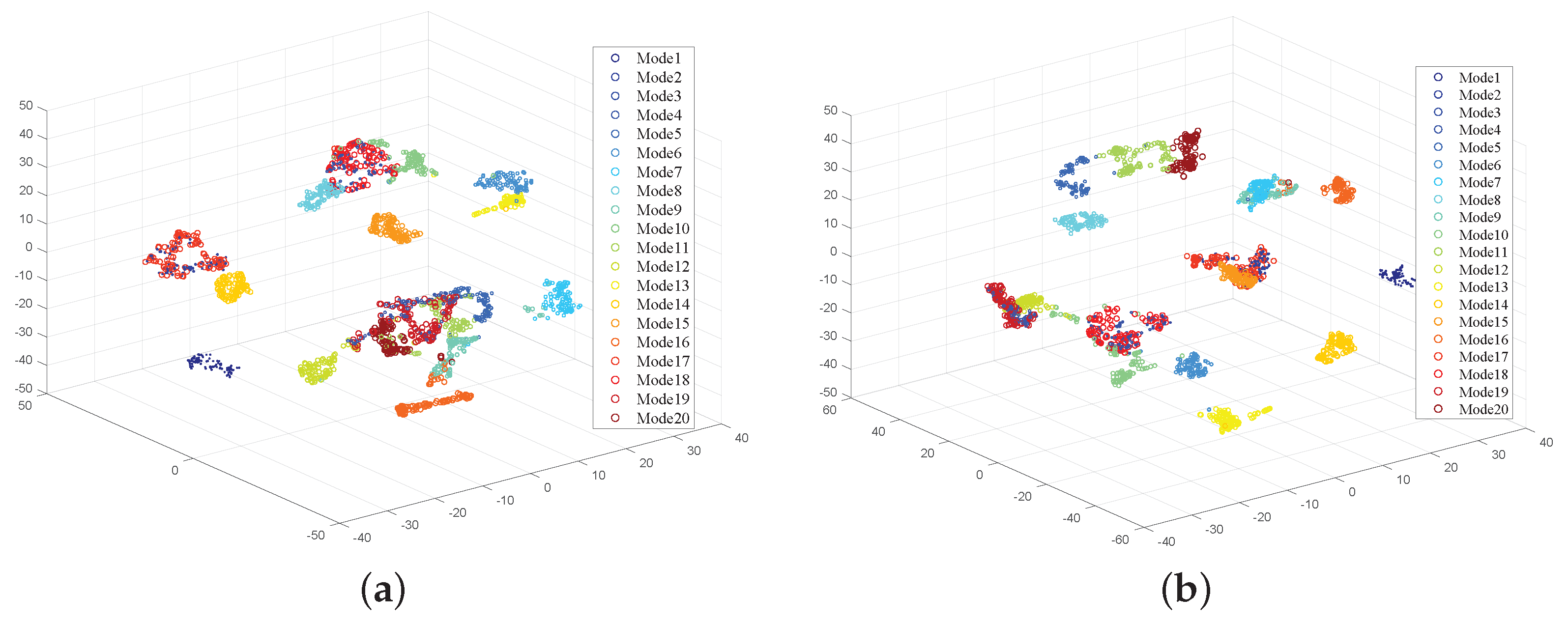
Figure 10 shows the t-SNE visualization results of features extracted by implementations of NSGA+Kmeans and NSGA+ANN. It can be observed from the figure that features from the majority of work modes exhibit clear distinguishability, while there is some overlap in features from a few minority modes.
4.4. Performance with Different Class Numbers
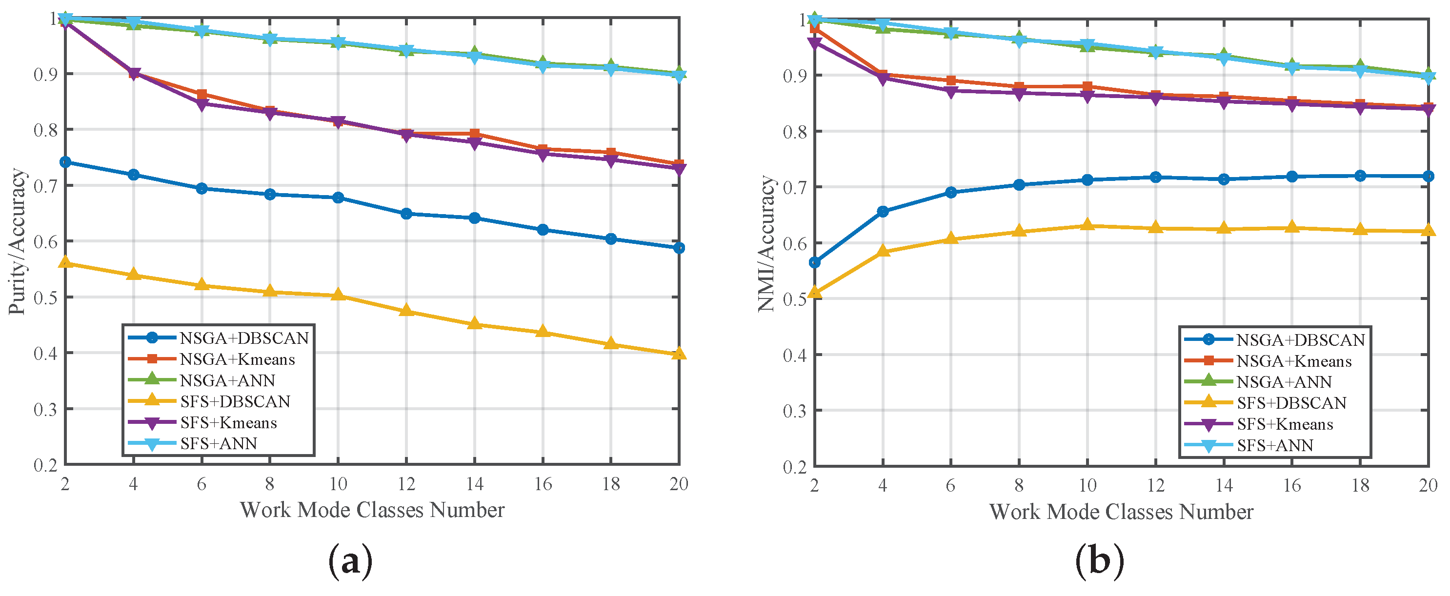
When comparing the effects of different implementations under various MFR work mode classes, Hybrid Scenario 4 was selected as the dataset. Two to twenty work mode classes were randomly selected from the dataset for each experiment.
Due to the different adaptability of different features to various classes, there is some fluctuation in the decreasing trend.
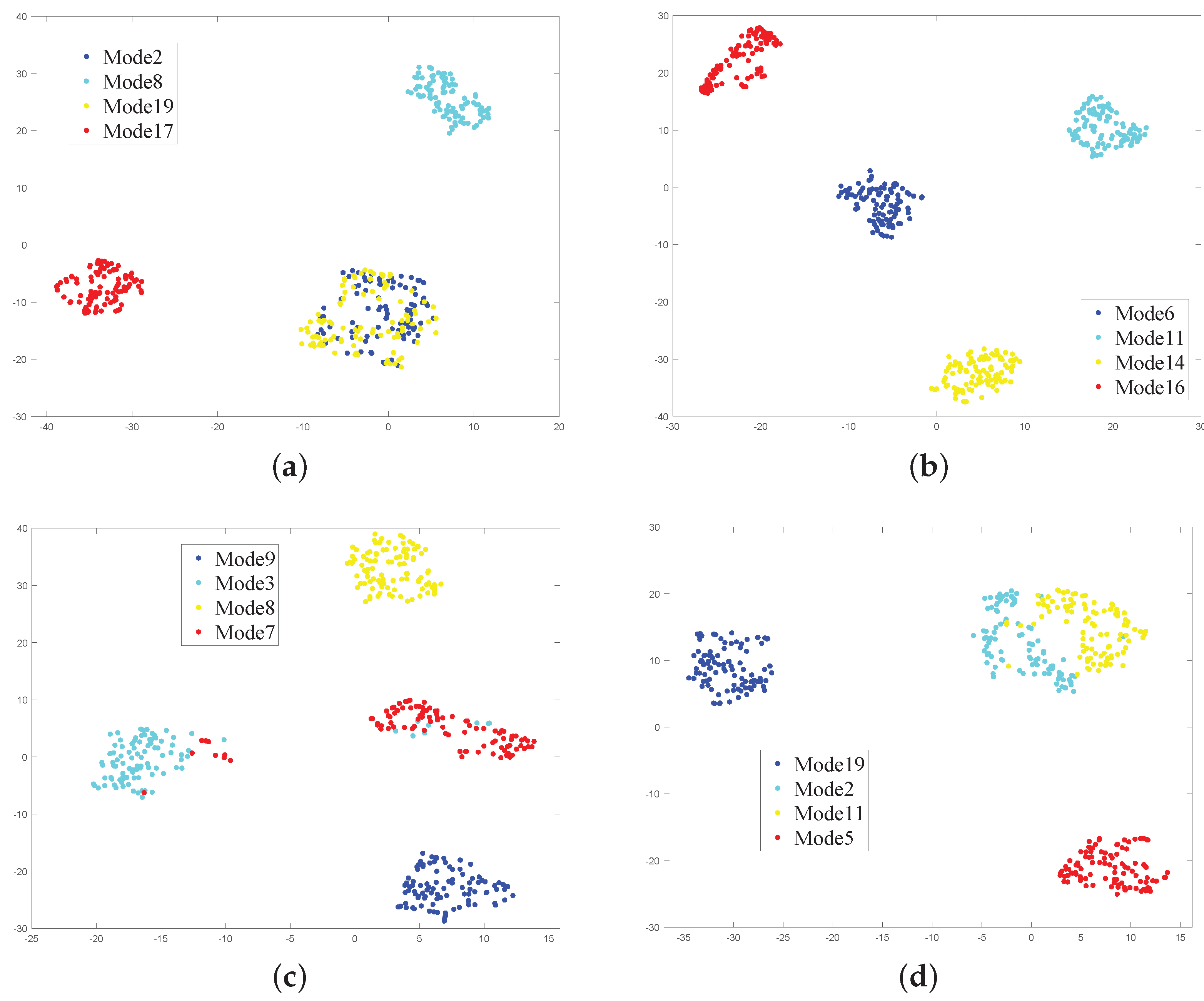
Figure 11 illustrates the feature visualization when randomly selecting 4 working mode classes multiple times. It can be observed from the figure that the distinctiveness of features varies when different classes are randomly sampled. The selected features showed poor adaptability to mode2, mode8, mode19 and mode17. Therefore, 100 tests were conducted randomly for each work mode class number, and the averages were taken as the final results. The experimental results are shown in
Figure 12. It can be observed from the figure that as the number of work mode classes increases, the overall performance of each implementation shows a decreasing trend.
Similarly, the NSGA+Kmeans implementation exhibits the best performance among clustering implementations, achieving purity of over 73.46% and NMI of over 84.28%. On the other hand, the SFS and DBSCAN implementation performs the worst, with a minimum purity of 39.65% and an NMI of 50.93%.
4.5. Performance Validation with Measured Signals
In fact, it is not convincing to evaluate the work mode recognition capability of these implementations only by testing them on simulated datasets. We used a radar simulator to generate signals and transmit them into space through a horn antenna, measuring 7 classes of the radar work mode to form the measured dataset. The PRI ranged from 378 to 1728
, the PW ranged from 16 to 93
, and the RF ranged from 2750 to 9780
. The elevation angle of the receiving antenna was approximately 10 degrees. The feature set selected in
Section 4.2 was used for the work mode recognition of the measured signals.
Figure 13 presents the recognition performance of different implementations. Both NSGA + ANN and SFS + ANN demonstrated satisfactory supervised recognition performance, achieving an almost 100% accuracy. As for the clustering methods, NSGA + Kmeans remained the best-performing approach, with clustering purity and NMI of 86.96% and 90.10%, respectively. The relatively poorest-performing approach, SFS + DBSCAN, had clustering purity and NMI of 73.19% and 82.69%, respectively. The proposed feature extraction and clustering framework and the selected feature set exhibited good work mode recognition capability.
5. Conclusions
With development in optimization theory, computation ability, and software-defined system architecture, MFR work modes with unseen modulations and modulation parameters emerge persistently. Unsupervised clustering of an MFR pulse sequence become urgent and important for electronic reconnaissance systems.
In this paper, a unified clustering framework is established for multivariate MFR time series and feature selection is conducted on a large number of time series features. Based on the existing advancements in time series research and the machine learning community, in this paper, features extracted through autoencoder-based deep learning, multidimensional time series features, and manually crafted PRI-type recognition features are considered and utilized in the traditional domain to form a feature set. Following that, NSGA-II and SFS feature selection algorithms are applied in conjunction with various clustering and classification methods to optimize features. Ultimately, the proposed framework and the chosen features are validated for effectiveness and superiority through extensive simulations on pulse sequence datasets.
Unsupervised recognition of MFR work modes plays a significant role in modern electromagnetic environments due to the increased degree of freedom of modern MFRs. There are many future works that can be investigated. First, more adaptive and accurate clustering methods are required to conclude the irregular scattering of different work modes in a high-dimensional feature space. Second sub-sequence clustering methods should be investigated with the findings in this study for clustering of pulse sequences with multiple consecutive radar work modes. Finally, probabilistic graphical models need to be investigated for the possible dependence between different variables in MFR applications.


