Abstract
With the development of artificial intelligence and deep learning, deep neural networks have become an important method for predicting the remaining useful life (RUL) of lithium-ion batteries. In this paper, drawing inspiration from the transformer sequence-to-sequence task’s transformation capability, we propose a fusion model that integrates the functions of the stacked denoising autoencoder (SDAE) and the Transformer model in order to improve the performance of RUL prediction. Firstly, the health factors under three different conditions are extracted from the measurement data as model inputs. These conditions include constant current and voltage, random discharge, and the application of principal component analysis (PCA) for dimensionality reduction. Then, SDAE is responsible for denoising and feature extraction, and the Transformer model is utilized for sequence modeling and RUL prediction of the processed data. Finally, accurate prediction of the RUL of the four battery cells is achieved through cross-validation and four sets of comparison experiments. Three evaluation metrics, MAE, RMSE, and MAPE, are selected, and the values of these metrics are 0.170, 0.202, and 19.611%, respectively. The results demonstrate that the proposed method outperforms other prediction models in terms of prediction accuracy, robustness, and generalizability. This provides a new solution direction for the daily life prediction research of lithium-ion batteries.
1. Introduction
Lithium-ion batteries are widely used in cell phones, electric vehicles, and other industries [1]. Due to their high energy density, long cycle life, fast charging and discharging, and low cost, lithium-ion batteries are the preferred choice for electric vehicles [2]. However, lithium-ion batteries contain flammable organic solvents and corrosive electrolyte salts in their electrolyte, and overcharging can lead to damage to the device, so it is important to predict their health to prevent overcharging and discharging [3]. The life of a lithium-ion battery is affected by the number of charge cycles, temperature, and other factors [4]. Accurately predicting RUL is critical to ensuring equipment reliability, extending battery life, and reducing replacement costs for electric vehicles and energy storage systems [5].
Currently, there are two main RUL prediction methods for lithium-ion batteries: statistical modeling methods and machine learning methods [6]. Statistical modeling methods use sample data to build regression models that make predictions based on physical quantities such as capacity degradation, temperature, and voltage. For example, Xu et al. [7] used a state-space model to predict RUL by integrating Expectation–Maximization (EM) and Extended Kalman Filter (EKF) algorithms to enable parameter and state updating. In addition, Hu et al. [8] used a simplified electrochemical model and the Moving Horizon Estimation (MHE) framework for the condition monitoring of batteries. However, statistical modeling approaches have limitations due to complexity, low dynamic accuracy, and imperfect electrochemical simulations; therefore, applying machine learning methods on large historical datasets is more suitable for predicting the RUL of lithium-ion batteries.
Machine learning ranges from time series methods, artificial neural network methods (ANN), and deep learning (DL) methods, among others. Zhou et al. [9] decoupled degradation trends and capacity regeneration from state of health (SOH) time series through empirical mode decomposition (EMD), which was combined with the autoregressive integrated moving average (ARIMA) method and integrated to obtain the final prediction results. Time series forecasting methods have some problems in predicting RUL values and dependence on the training set. In contrast, DL, as a newer machine learning method, solves the above problems well [10]. DL algorithms such as recurrent neural networks (RNNs), deep neural networks (DNNs), and autoencoders can approximate complex nonlinear models and achieve accurate predictions. Jia et al. proposed a multi-scale RUL and SOH prediction method combining wavelet neural network (WNN) and untraceable particle filter (UPF) models. The battery capacity degradation data were decomposed into low-frequency trends and high-frequency fluctuations by discrete wavelet transform (DWT), and the WNN-UPF model was utilized to predict the long-term RUL and integrate the high-frequency fluctuation data to estimate the short-term SOH [11]. Ren et al. [12] proposed an integrated approach combining autoencoder and DNN to improve the prediction accuracy of RUL for lithium-ion batteries. All these studies have significant advantages in terms of computational cost and performance metrics.
Although neural networks based on RNN frameworks have proven to be effective in modeling continuous data, they still face some challenges such as long training times, high computational burden, and long-term dependencies. However, in the practical application of RUL prediction for lithium-ion batteries, networks that can perform in parallel and retain spatial location information of the input data are crucial [13]. In contrast, CNNs are insensitive to the length of the input sequence and can easily achieve parallel computation [14].
The Transformer architecture provides a potential solution to the above problem by using fully connected networks and a well-designed attention mechanism [15]. Zhou et al. [16] proposed a location-encoded attention mechanism, CNN, to solve this problem, while taking advantage of the parallelization of CNNs to improve the accuracy of battery RUL prediction. Chen et al. [17] developed a new Transformer structure for processing battery capacity data by learning useful features through input reconstruction sequences. However, the pure Transformer model is relatively complex and requires a lot of computational resources and time for training. Therefore, it may lead to high computational costs during the prediction process and is not suitable for real-time RUL prediction. According to further research, it has been shown that the Transformer model is very dependent on the quality of the original dataset. This sensitivity to outliers and noise can cause the model to overreact to data fluctuations in real-world applications, thus affecting the stability of the predictions. A stacked denoising autoencoder (SDAE) is a deep learning model suitable for neural networks and specialized for dealing with data quality problems [18]. It has advantages in dealing with outliers and noise and is capable of efficiently processing large-scale data in parallel. Liu et al. [19] proposed an intelligent fault diagnosis method that combines Local Mean Decomposition (LMD) and the SDAE model. It is able to adaptively learn fault features, which improves the effectiveness and robustness of the method.
In order to solve the fundamental problem that traditional Transformer models are too dependent on raw data, this paper proposes a method for accurately predicting the RUL of lithium-ion batteries in the presence of random discharges. By combining the SDAE with the Transformer architecture, it can improve the prediction accuracy of the RUL of lithium-ion batteries and shorten the training time of the prediction model. The contributions and innovations of this research are as follows:
- (1)
- In this study, a novel architecture integrating noise reduction and prediction is constructed by integrating an SDAE into the Transformer model structure. By reducing noise and extracting important features, the new structure improves the reliability and availability of raw data. In addition, for longer time series, it reduces the computational complexity of the Transformer model and improves the model prediction accuracy.
- (2)
- This study focuses on the data from the downscaled fusion of random discharge conditions and PCA methods. It focuses more on the performance degradation of lithium-ion batteries during real-world use than existing lithium-ion battery research. The experimental data come from the NASA lithium-ion battery random-use dataset, which contains a wide range of battery operating states and real-world conditions, which makes the experiment more credible and reliable.
- (3)
- In order to verify the applicability and robustness of the model, this study uses several different health factors for experimental validation. By training the prediction of these different health factors, the results marked that the reliability and utility of the model are further enhanced. It provides sufficient support and assurance for the practical application of the model in various scenarios.
2. Materials and Methods
To address the problems of existing RNN-based methods, we design a deep learning neural network architecture. The architecture mainly consists of three parts: health factor extraction, SDAE–Transformer model, and RUL prediction.
2.1. Stacked Denoised Autoencoder
Data denoising is necessary to improve the accuracy and effectiveness of training models. Lithium-ion battery random use datasets contain a lot of noise. They need to be denoised before they are provided to the prediction model to ensure the stability and robustness of the model. Therefore, appropriate methods are needed to remove noise from the data and ensure that the model can be trained using high-quality input data.
In this section, we propose an approach based on SDAE, which extends from the denoising autoencoder (DAE). DAE [20] is an extended version of the autoencoder (AE). It introduces noise into the input data and trains the network to reconstruct the original data without noise, thereby learning a more robust and resilient feature representation. To solve this problem, multiple DAEs can be used to reconstruct inputs containing noisy data [21]. The SDAE is engineered to acquire multi-level abstract features of the data [22]. This is achieved by progressively assembling multiple denoising autoencoders to build a depth representation. The basic concepts are trained layer by layer to extract more abstract and advanced features in the data, enhancing the ability of the model to represent and abstract the data.
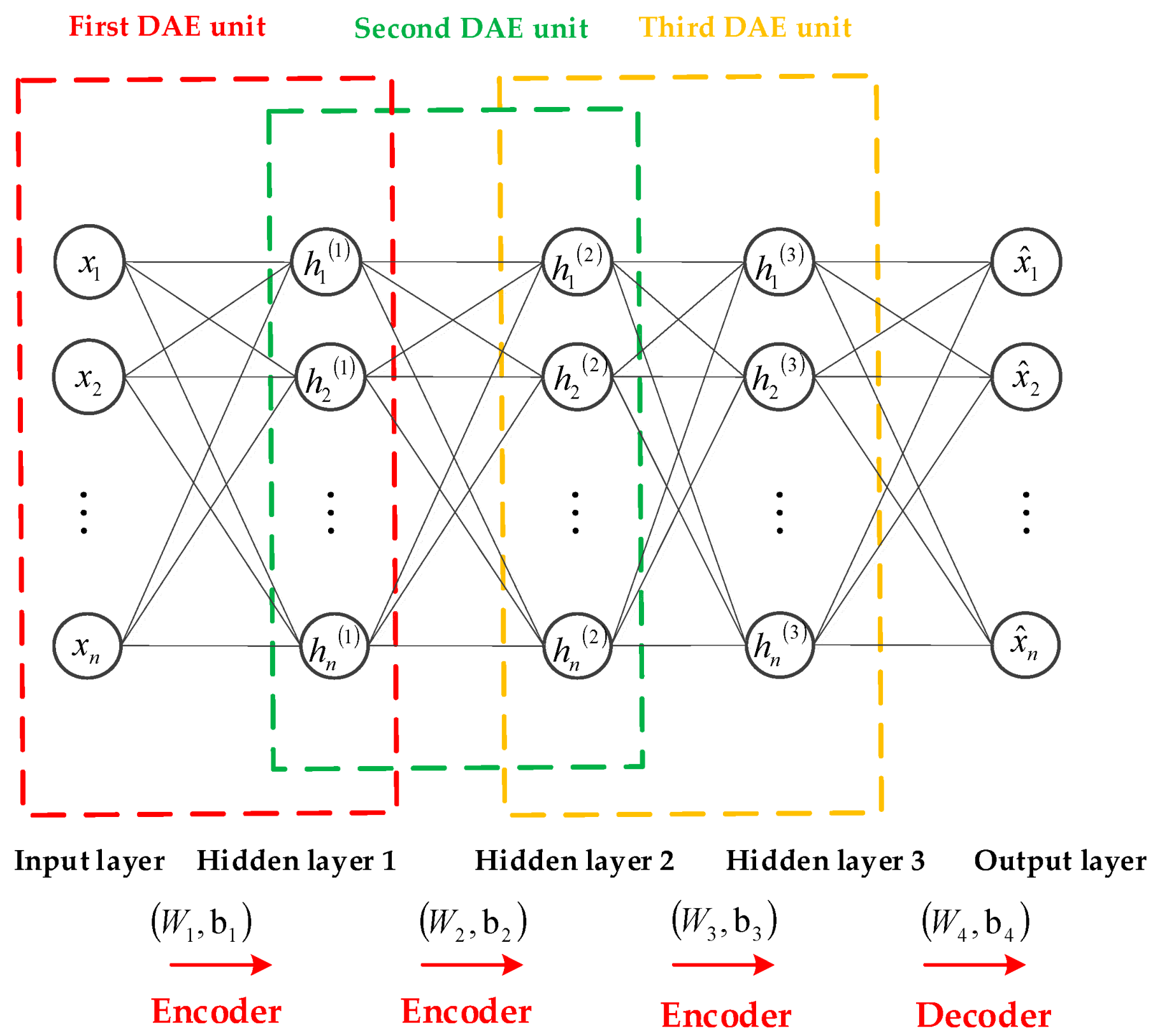
The following describes in detail the specific steps to build an SDAE with a three-layer hidden layer structure:
We pre-train the first DAE unit. The input vector is , where is the total number of samples. The loss vector y is obtained by adding Gaussian noise to . Then, the encoder performs a mapping conversion from the vector to the output representation by using an active function. The calculation expression is as follows:
where is the weight from the input layer to the hidden layer, and is the bias of the hidden layer. is the Sigmoid function.
Decoding is the procedure of mapping from a high-dimensional space into a high low-dimensional space and reconstructing the input sample into , as in the following Equation (2):
The minimum mean squared error is used as the lost function and the gradient descent method is utilized for updating the weight vector and bias item . The calculation is as follows:
After pre-training, the output layer and its corresponding weights and biases are removed, and only and of the input and hidden layers are retained. Then, the hidden layer of the first DAE unit is used as the input of the second DAE unit. The second DAE unit is trained in the same way, and so on to the third. After the pre-training of the three DAE units, the last thing to be performed is the overall inverse tuning training. The structure is shown in Figure 1.
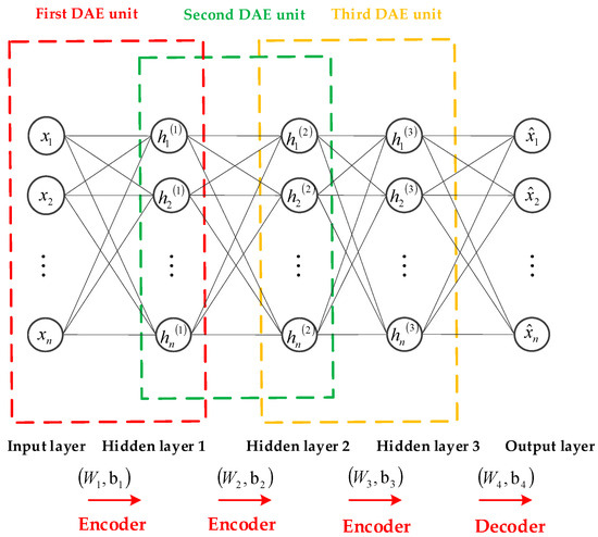
Figure 1.
Stacked denoising autoencoder structure diagram.
2.2. Transformer Model
In 2017, Google proposed the Transformer model, employing an encoder–decoder architecture and replacing the traditional RNN structure. The model replaced the traditional RNN structure with a self-attention mechanism, achieving superior performance [23]. This marked the first model to rely entirely on self-attention mechanisms for computing input and output representations. The encoder is employed to process the source language, while the decoder is used for the target language. In this study, the encoder of the Transformer model was utilized to analyze the operational records of lithium-ion batteries and predict the declining trend in battery capacity during random discharges.
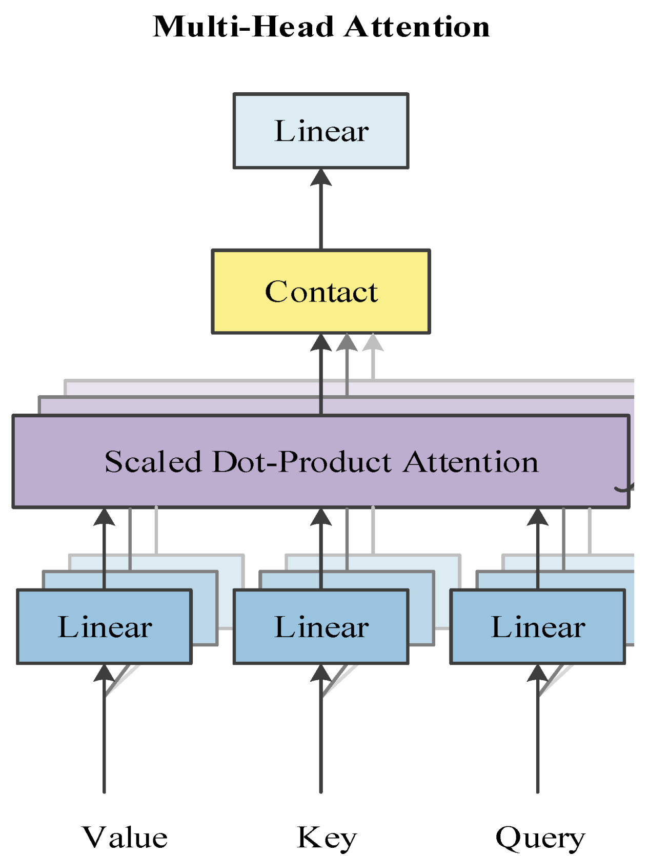
The concept of multi-head attention involves mapping the same Query, Key, and Value to different subspaces for attention computation. This process ultimately merges the information from these different subspaces. This helps reduce the dimensionality of each head and prevents overfitting. The structure is illustrated in Figure 2.
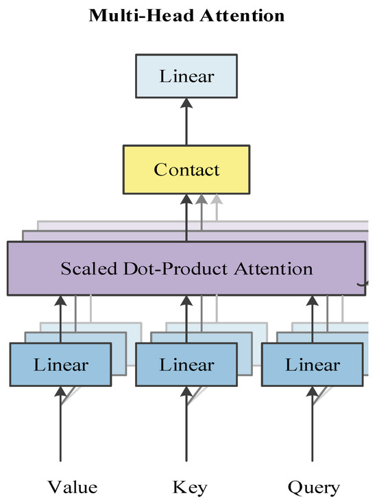
Figure 2.
Multi-headed attention mechanism structure diagram.
Each set of attention is used to map the input to a different subrepresentation space, which allows the model to focus on different locations in different subrepresentation spaces. The whole computational process can be represented as the following:
where . , , and are three vectors obtained by mapping the input sequence by three linear mapping layers. is the number of attention heads, is denoted as the model dimension, is the dimension of the Key, and is the dimension of the Value. The is the final output weight matrix obtained by dimensionality reduction, respectively. The Contact function represents the concatenation function, which combines the output results of all heads.
With multiple attention, we maintain separate Query, Key, and Value weight matrices for each group of attention, resulting in different Query, Key, and Value matrices. As shown in Equation (5), , , , denote the weight matrices corresponding to the , , and vectors of the i-th head.
A positional feedforward network is a fully connected feedforward network (FNN), where each positional feature individually passes through this identical feedforward neural network. It consists of two linear transformation layers with a ReLU activation function in the middle, which can be expressed as:
where , , , are the weights and biases of the two linear transformations.
Each sublayer of each encoder in the encoder structure has a residual connection and then performs a layer normalization operation. The whole computation can be represented as follows:
Since the Transformer model does not have a built-in mechanism for processing positional information like recurrent neural networks (RNNs) or convolutional neural networks (CNNs). Therefore, positional encoding is used to add additional information for each word or position in the input sequence so that the model can capture information about the position of the word in the input sequence. The mathematical formulas are as follows:
where denotes the position of the word in the input sequence, and i denotes the index of the position encoding matrix. The position encoding matrix thus computed is summed with the word embedding matrix to obtain an input vector containing positional information.
Typically, this position encoding method is standard practice in the Transformer model. However, other positional encoding methods, such as absolute positional encoding, can be tried to adapt to different tasks and data characteristics. In some specific scenarios, position encoding may need to be adapted to meet the needs of a particular task.
2.3. SDAE–Transformer Model Prediction
In our model, there are two tasks: denoising and prediction. We propose an objective function to solve these two tasks. The learning process optimizes both tasks in a unified framework that predicts the unknown capacity. A complete connectivity layer is used to map the representation of the final Transformer unit to obtain the final prediction , as shown in Equation (10):
where , , , and denote the mapping functions of weights, biases, inputs, and map function of the prediction layers, respectively.
The experimental procedure consisted of several key steps. First, historical battery data were collected, which contained valuable information reflecting trends in battery degradation. From these data, health factors are extracted as indicators of battery degradation. Second, the extracted health factors are normalized to ensure comparability and consistency. The third step is to integrate the SDAE module into the encoder and decoder components of the Transformer architecture. This integration produces the SDAE–Transformer model, which combines the noise reduction and feature extraction capabilities of the SDAE. Finally, the trained model is used to predict the RUL of the battery and optimize the model parameters in the process. Figure 3 visually depicts the algorithmic framework and overall flow.
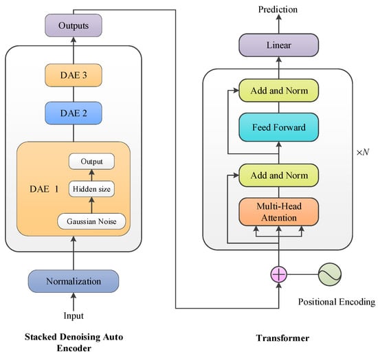
Figure 3.
The graphical representation of the SDAE-Transformer model architecture.
3. Experimental Design
3.1. Data Description
The internal structure of lithium-ion batteries is highly intricate, necessitating corresponding parameter acquisition during the research process. The random battery datasets from the Ames Excellence Prediction Center of the National Aeronautics and Space Administration in the United States were employed in this study due to their abundant and diverse battery test data [24]. There are seven datasets in the dataset, and the data contain some spurious data, including incorrect temperature measurements (RW2, RW3, and RW18), outliers due to experimental noise (RW9), non-normal step durations (RW16 and RW17), and incorrect current measurements (RW19) [25]. These anomalies may negatively affect data analysis and interpretation. One of the groups of 18,650 lithium-ion batteries (RW3, RW4, RW5, and RW6) was selected for the experiments since the study in this paper is not temperature-dependent. The data were run continuously by repeatedly charging to 4.2 V and then discharging to 3.2 V. Discharge currents ranged between 0.5 A and 4 A and the order of discharge was randomized. This type of discharge profile is referred to here as a random walk (RW) discharge. After every 50 RW cycles, a series of reference charging and discharging cycles were performed to provide a reference baseline for battery state health. The experimental data use random discharge currents to vividly simulate the uncertainty of daily battery use. This better represents typical battery usage scenarios and is close to real-world usage conditions.
3.2. Extraction of Health Factors
The lithium-ion battery constitutes a sophisticated electrochemical system, wherein irreversible lithium-ion deposition and subsequent decay in battery capacity take place during charge–discharge cycling. Direct quantification of battery capacity to elucidate its operational health is unfeasible. However, the aging status of the battery can be indirectly inferred through other factors such as charge–discharge voltages, currents, temperature, and time. These factors impact the electrochemical processes within the battery, leading to changes in its internal structure and performance over time. By monitoring and analyzing these factors, it is possible to gain insight into the health and remaining lifespan of the battery, allowing for the development of predictive models and strategies to optimize battery usage and longevity.
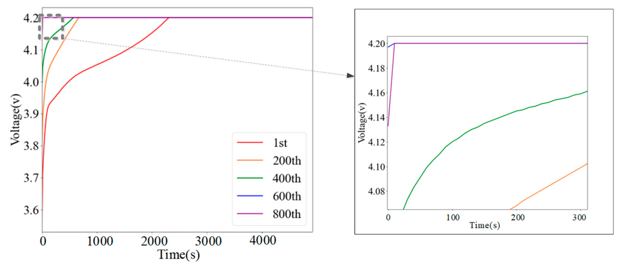
In the random walk (RW) mode of battery cycling under the NASA datasets, there are two phases. One of these is the “charging (after random walk discharge)” phase, where the current is adjusted to maintain the battery output at 4.2 V during the charging process, until the battery current drops below a lower threshold. Depicted in the two figures shown in Figure 4 are the voltage profiles corresponding to different cycles of the battery during constant current and constant voltage charging. We have given a zoomed out view of the details. It can be seen that as the number of cycles of the battery increases, the aging speed of the battery accelerates and the time to reach the maximum threshold voltage of constant voltage charging is gradually shortened. The time for the battery to reach the cutoff voltage (4.2 V) in the first cycle is about 2310s, while the cutoff voltage can be reached instantaneously after the 600th and 800th cycles. Therefore, the battery capacity calculated from the charge saturation time is called the health factor H1. Its mathematical formula is expressed as follows:
where is the saturation voltage with a value of 4.2 V, is the charging time of the -th cycle in hours, and is the current measured at the i-th RW’s cycle τ moment.
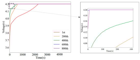
Figure 4.
Voltage curve of the battery during partial cycles of charging.
Figure 5 shows the decay curves of battery capacity during constant-current and constant-voltage charging. Looking at the whole cycle, the capacities of different battery monomers all decrease over time, which is consistent with the capacity decay trend of conventional lithium-ion batteries during actual use. It is worth noting that, due to the complex physical and chemical processes of batteries, the capacity curves of batteries may show different fluctuation amplitudes under the same conditions, a phenomenon that is also consistent with the daily use of batteries. Therefore, H1 can be used as a characteristic input for predicting the RUL of lithium-ion batteries.
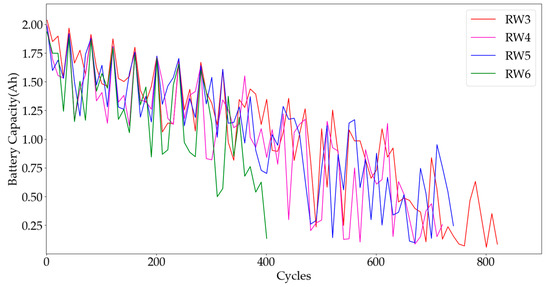
Figure 5.
Degradation curves of battery capacity in the charging phase after random discharge.
The discharge capacity in “discharge (random walk)” refers to the amount of power released by the battery during the random walk phase using a random sequence of discharged loads, which can be found by integrating the current and time of the battery during discharge. The aging of the battery leads to a gradual reduction in both the actual available capacity and the discharge time, as well as the loss of lithium. Figure 6 shows the discharge capacity of one RW cycle. The discharge capacity of a complete randomized discharge cycle can be obtained by summing the integrals of the current and time of 50 RW cycles with the following equation:
where is the discharge capacity obtained in the random discharge cycle, is the time of the -th RW cycle, and is the current measured at moment τ of the cycle of the -th RW.
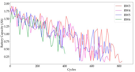
Figure 6.
Battery degradation capacity during the discharge (random walk) phase.
Meanwhile, we obtained the complete random discharge cycle discharge capacitance of all four batteries involved, and it can be seen from Figure 6 that the discharge current is different at different times in the same RW cycle, which corresponds to the actual battery usage. Therefore, H2 can be used as a characteristic input for predicting the RUL of lithium-ion batteries.
3.3. PCA Fusion Health Factor
3.3.1. Assessment of Health Factor Correlation
The Pearson correlation coefficient (PCC) is a widely utilized linear correlation measure in statistical analysis [26]. It is employed to quantify the influence of a health factor, denoted as γ, on the capacity of the battery. The range of the γ value extends from −1 to 1. Within this interval, a larger absolute value signifies a higher degree of correlation. In other words, a higher absolute value implies a stronger correlation. The formula is as follows:
where is the sequence length, is the extracted health factor, and is the battery capacity.
and
denote the average values of the health factor and the battery capacity.
Table 1 displays the magnitude of the PCC between the battery capacity at the saturation time of the charging voltage and the battery capacity at random discharge for four lithium-ion batteries. It is evident from the table that the Pearson correlation coefficient values for this set of batteries are greater than or equal to 0.995, indicating a very strong correlation between the two variables. This strong correlation suggests a linear relationship between the two sets of health factors.

Table 1.
Battery health factor correlation assessment form.
3.3.2. PCA Fusion Health Factor
These two extracted health factors are highly correlated, resulting in redundant information. Therefore, we used principal component analysis (PCA) to transform these correlated health factors into a set of uncorrelated principal component health factor H3, thus reducing the dimensionality of the data and optimizing the extracted health factors [27]. The Kaiser–Meyer–Olkin Measure of Sampling Adequacy (KMO) and Bartlett’s test were first performed to determine whether principal component analysis could be conducted. For the KMO value, 0.8 is considered very suitable for principal component analysis, between 0.7 and 0.8 is generally suitable, between 0.6 and 0.7 is not very suitable, between 0.5 and 0.6 indicates being poorly suitable, and under 0.5 indicates being extremely unsuitable. If the p value in Bartlett’s test is less than 0.05, the original hypothesis is rejected, indicating that principal component analysis can be conducted. If the original hypothesis is not rejected, the variables may provide independent information and are not suitable for principal component analysis.
From Table 2, the results of the KMO test show that the value of KMO is 0.821, which is very suitable for principal component analysis. Meanwhile, the results of Bartlett’s spherical test show that the significance p is 0, which presents significance at that level, rejects the original hypothesis that there is a correlation between the variables, and the principal component analysis is valid.
Table 2.
KMO and Bartlett sphericity tests.
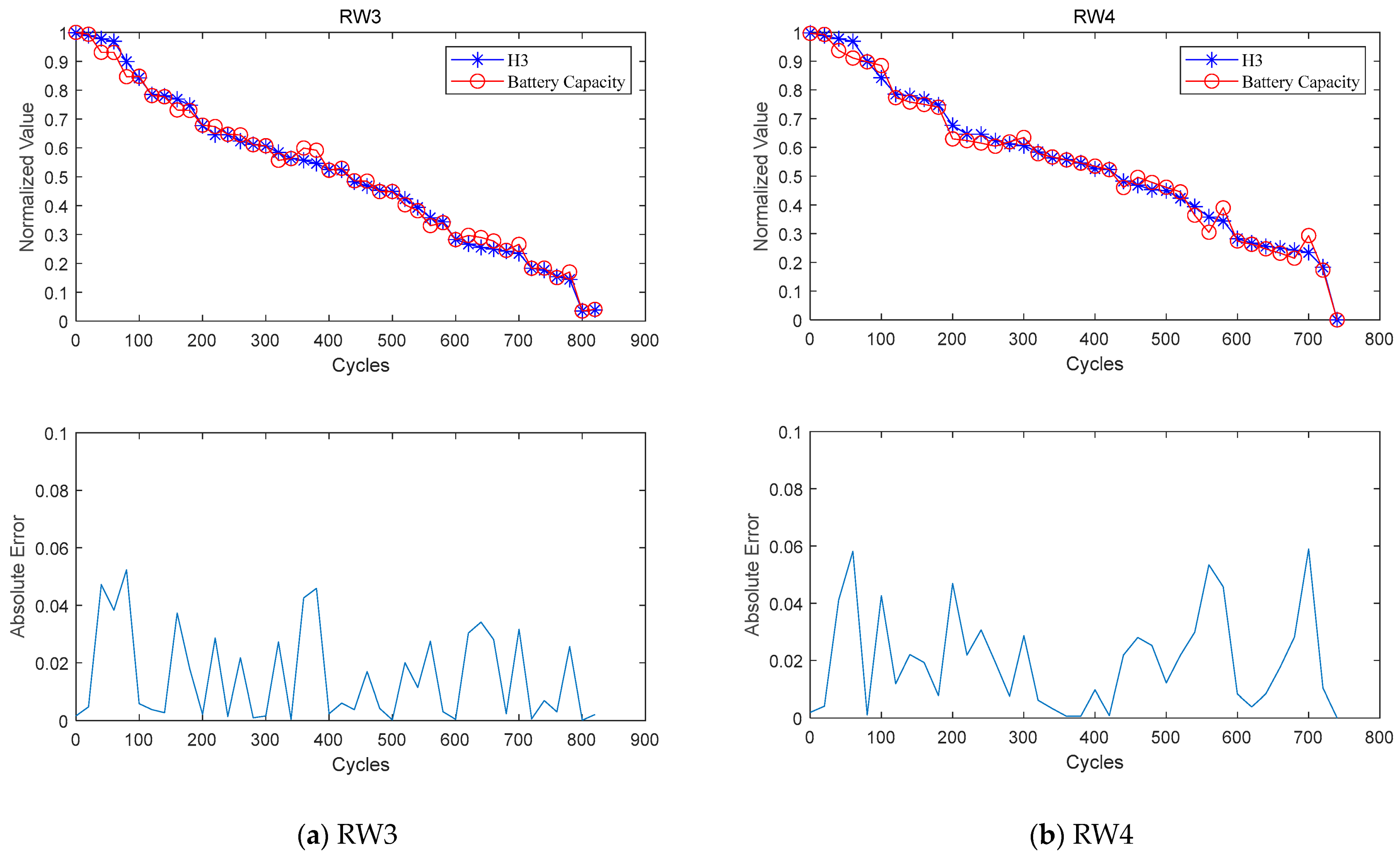
In order to make the curve trend clearer, the H3 and battery capacity are normalized and using Equation (14):
where X denotes normalized data, x denotes raw data., and and are the minimum and maximum values of the x, respectively.
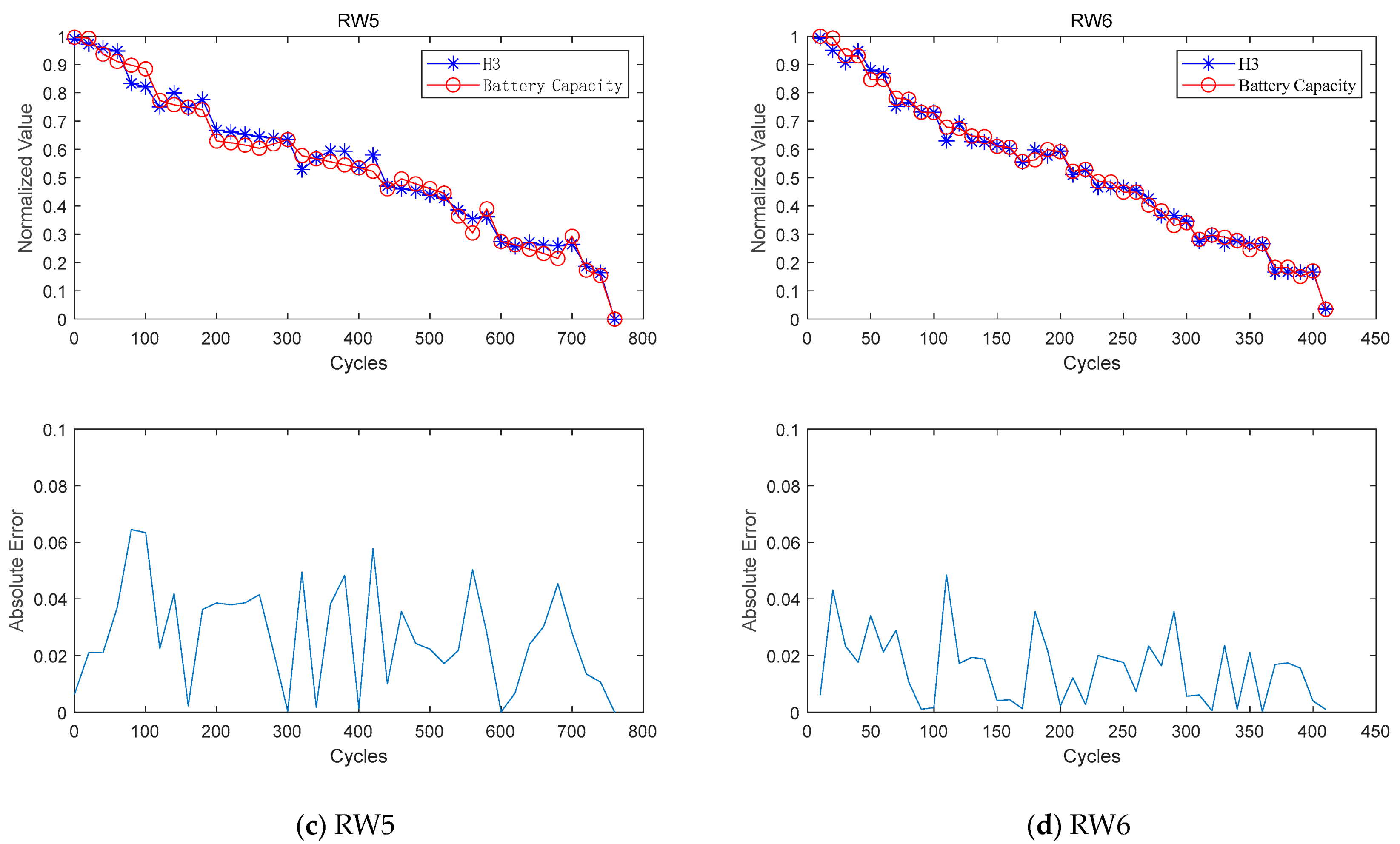
Figure 7 shows the normalized value curve between H3 and battery capacity. As shown in Figure 7, the error range between the fused health factor H3 and the reference capacity of the four lithium-ion batteries is within 0.05. This indicates a strong correlation between the health factor and battery capacity for the four batteries. Especially for RW5 batteries, the H3 curve matches well with the capacity decay curve. Therefore, the health factor H3 after PCA fusion can also be used as an input to the lithium-ion battery RUL prediction model.
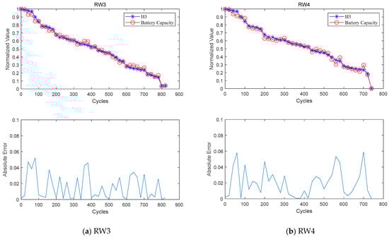
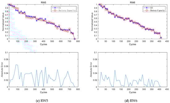
Figure 7.
Battery capacity versus fusion health factor H3 normalized and absolute error relationship curves for four batteries.
3.4. Experimental Setting
3.4.1. Problem Statement
The primary objective of this research methodology is to predict the RUL of lithium-ion batteries based on historical data. The prediction of remaining useful life involves the application of certain mathematical techniques to the battery’s historical data to calculate the remaining life of the battery. The storage life of a lithium-ion battery represents the time required for the battery to degrade to a certain extent under static or non-operating conditions [28,29]. On the other hand, the usable lifetime of a battery refers to the number of cycles experienced under specific charging and discharging conditions [30]. This degradation leads to the battery’s current available capacity to a predetermined failure threshold, as described with Equation (15).
where is the number of lithium battery reference discharge cycles and is the number of lithium battery actual discharge cycles.
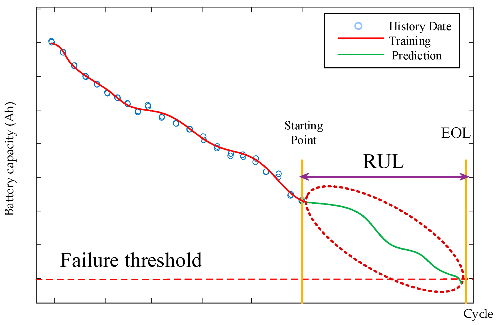
For batteries, the definition of End of Life (EOL) is closely related to the battery capacity. When the remaining capacity of the battery reaches 70–80% of its initial capacity, it is considered to have reached the end of its life, and a measurement can only be obtained from discharge cycle data [31]. Figure 8 provides an example of predicting RUL based on the datasets.
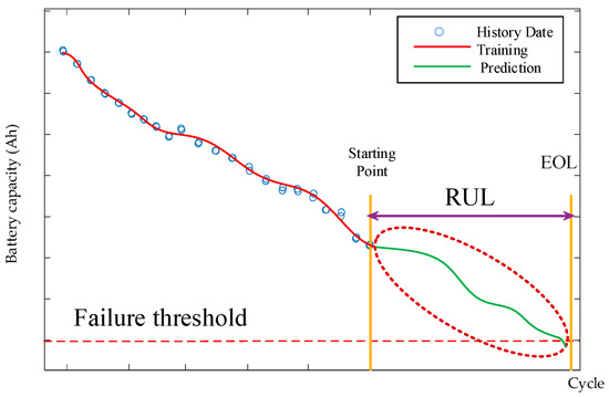
Figure 8.
Schematic of battery capacity degradation of lithium-ion batteries.
3.4.2. Evaluation Indicators
We chose four evaluation metrics to assess model performance, i.e., Relative Error (RE), Mean Absolute Error (), Root Mean Square Error (), and Mean Absolute Percentage Error (). Four evaluation metrics are defined as follows:
where n is the sequence length, is the true value in the RUL prediction, and is the predicted value in the RUL prediction.
Then, one battery was randomly selected as a test set and the other three batteries were used for training sets.
3.4.3. Parameter Setting
There are six key parameters in the model used in this experiment: sampler size (), learning rate (), depth () and hidden layer size () of the Transformer, learning regularization (), and the proportion of each task (). The value of “m” can be set to approximately 5% of the length of the sequence, and it is fixed at 16 for the NASA datasets. The rest of the parameters were determined by a grid search on the validation error: is chosen from [10−4, 5 × 10⁻⁴, 10−3, 5 × 10⁻³, 10−2]; is chosen from [2, 4, 8, 16]; is chosen from [1, 2, 3, 4]; is chosen from [10−6, 10−5, 10−4, 10−3]; is set from (0, 1]. The optimal set of parameters for the four models is presented in Table 3.
Table 3.
Optimal parameters of the four models.
Battery capacity was estimated using a GeForce RTX 3050 laptop graphics processor with NVIDIA. All code runs on Pytorch 1.13.1, Python 3.8, and the win11 operation system.
4. Results and Discussion
In this section, evaluation indicator results for battery RUL estimation based on the Transformer model with a stacked noise-reducing self-encoder are given and its performance is compared with other state-of-the-art neural network methods such as MLP, LSTM, and Transformers.
4.1. Model Online Validation
We first validate the overall prediction performance of different batteries with different health factors. We selected a subset of batteries from the datasets and used a cross-validation method to randomly select one battery for testing, while the rest were used for training, and finally predicted the RUL of the batteries. For example, in the first experiment, we used batteries RW4, RW5, and RW6 as training batteries and RW3 as the test battery. The results of the final evaluation metrics (, and ) for these four sets of experiments are shown in Table 4.
Table 4.
Evaluation index values of batteries.
According to Table 4, we can calculate the mean values of the three evaluation indicators of the three health factors: is 0.170, is 0.202, and is 19.611%. The results show that the SDAE-Transformer model has high prediction accuracy and can accurately reflect the actual value. The values of , and are close to each other, indicating that the prediction error of the model is relatively stable with no obvious deviation. As shown in Table 4, we observed that our model exhibited substantial accuracy and stability across different individual batteries. Our model consistently and accurately predicted their performance. This indicates the strong generalization capability of our model, enabling it to adapt to diverse individual batteries. Furthermore, we observed minimal discrepancies between the model’s predictions and the actual data. This implies the model’s adeptness at capturing the performance characteristics and variation trends of the batteries, thus facilitating accurate predictions.
In battery prediction experiments based on different health factors, our optimization model similarly made equally accurate predictions for each battery. The results show that the SDAE-Transformer model is proficient in extracting key features from different health factors and effectively integrating these features to comprehensively analyze the RUL status of the battery. The SDAE-Transformer model effectively captures the nonlinear relationship between battery capacity and various health factors. In addition, it extracts valuable temporal information from the capacity sequences for accurate prediction.
By comparing and analyzing the predictive evaluation metrics of the three health factors in Table 4, we can draw the following conclusions: (1) The values of all evaluation metrics for H2 are higher than those for H1, possibly due to H2 being extracted based on random discharge, which more accurately reflects the battery’s health status under random discharge conditions. This also demonstrates that our model is more suitable for predicting battery remaining life in random states and can provide higher prediction accuracy. (2) Among the three health factors, H3 has the best predictive performance with the smallest values of , , and . This indicates that H3 possesses the superior capability to accurately predict the battery’s health status. When a singular set of feature sequences is presented to the network, the model may encounter challenges in accommodating the diverse fluctuations within these sequences, consequently constraining its predictive capability. In order to enhance precision, we integrate supplementary feature sequences to capture the battery’s dynamic changes. This allows us to establish global dependencies between different positions, successfully achieving the interaction of global information.
4.2. Effects of SDAE-Transformer Hidden Layer
In this section, we discuss the effects of hidden layers on the SDAE-Transformer model under different health factor input conditions. In the experiment, three evaluation indicators were used to evaluate it, and the results were shown in Table 5.
Table 5.
Effects of SDAE-Transformer hidden layer with different health factors.
The overall trend observed in Table 5 is that all evaluation metrics tend to increase and then decrease with an increase in hidden layers. The most probable explanation is that the Transformer’s restricted weight capacity hinders the assimilation of sufficient temporal information. Consequently, inadequate fitting occurs when the hidden size is too small. Conversely, when the hidden size is too large, the Transformer becomes burdened with an excess of weights for learning temporal information. According to the results in Table 5, when the number of hidden layer is 8, the value of each evaluation index is optimal.
4.3. Comparison with Other Advanced Methods
In order to validate the efficacy of the proposed SDAE–Transformer model, it was extensively compared with other data-driven approaches such as LSTM, MLP, and the Transformer.
MLP [32]: It is a feedforward neural network with simpler connectivity. With multiple fully connected layers, it is used to learn the dynamic and nonlinear degradation trends of the battery.
LSTM [33]: It is a temporal recurrent neural network that solves the long-term dependency problem present in general RNNs for learning degradation trends from input sequences.
Transformer [17]: It is a deep learning model based on the attention mechanism, which utilizes the self-attention mechanism to capture the dependencies between the positions in the input sequence, thus enabling the modeling and processing of sequence data.
Figure 9 illustrates the predicted values versus H3 health factor curves for the four models.
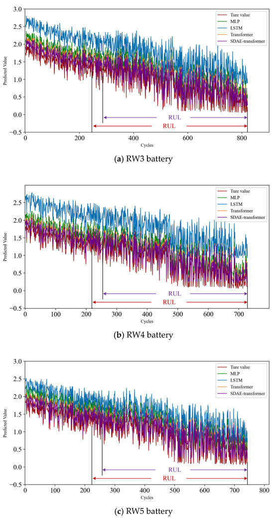
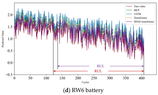
Figure 9.
Predicted and H3 value curves for the four prediction models.
Figure 9 shows that comparing the predicted and H3 curves, the SDAE-transformer model has the best performance and is closest to the actual values. This is attributed to its combination of SDAE and Transformer characteristics, enabling better learning and feature extraction of the battery RUL, thereby improving predictive accuracy. On the other hand, LSTM had the largest error. This may be due to the large datasets and high noise, making it difficult for LSTM to effectively capture complex long-term dependencies, resulting in significant prediction errors. The Transformer-based models exhibited reduced prediction errors as a result of the self-attention mechanism’s capacity to capture long-range dependencies within the sequence data. This enhancement contributed to improved predictive accuracy for RUL. In general, the models we proposed have shown superior predictive capabilities and greater precision in handling battery datasets that contain a substantial amount of noise and outliers. These findings highlight the effectiveness of our models in dealing with challenging data scenarios.
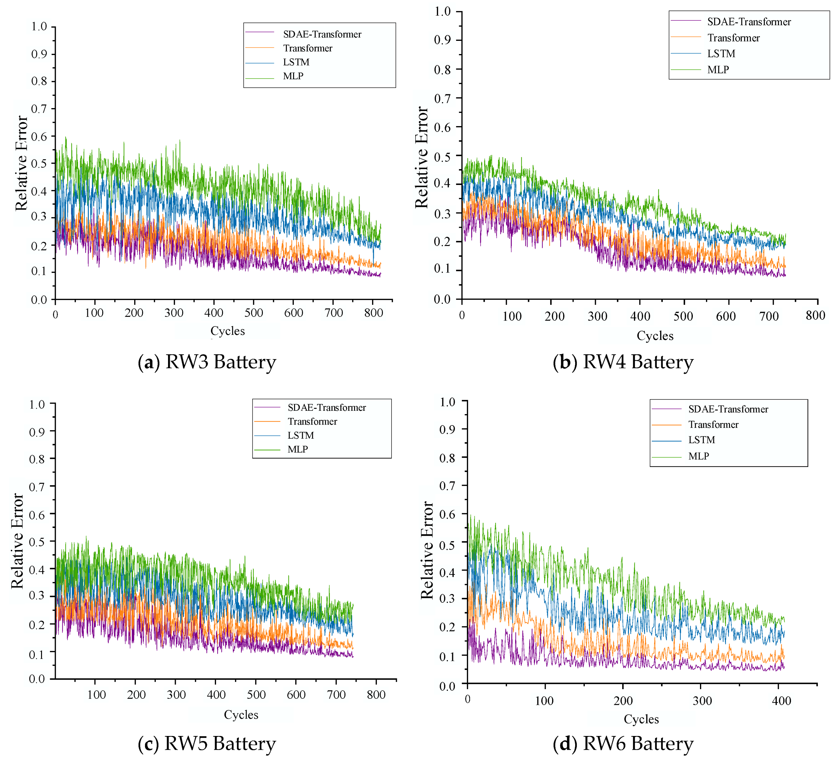
Figure 10 shows the RE results for the four batteries with the four different methods. The curves shows that the improved model achieves the lowest RE value in the predictive experiments for all four batteries, while the MLP model exhibits the highest RE value. Notably, the RE prediction curves during the early stages of the experiments exhibit varying degrees of fluctuation. This observation can be attributed to the limited historical data available and the insufficient understanding of the intricate and nonlinear degradation patterns exhibited by lithium-ion batteries in the initial phases of their lifespan. These factors can introduce inaccuracies in the predictions and result in noticeable fluctuations in the curves. Additionally, the collection of data under random discharge conditions can introduce noise and uncertainty, influencing capacitance measurements and data recording. As the model accumulates more data and gains experience, its understanding deepens, leading to improved prediction accuracy and stability. Consequently, the fluctuation in the prediction curves diminishes over time, and the model approaches a more stable performance.
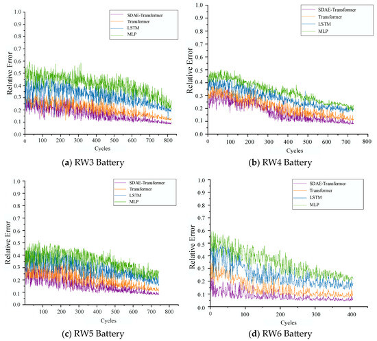
Figure 10.
Comparison curves of RE predictions for the four machine learning methods for each battery.
Figure 10 illustrates that the Transformer model demonstrates a lower degree of fluctuation in contrast to the MLP and LSTM models. This can be attributed to the inclusion of the self-attention mechanism. It enables comprehensive interactivity to model the interconnections between each position and other positions. As a result, this diminishes fluctuations in the curve. Furthermore, the Transformer model utilizes positional encoding to encapsulate positional information within the sequence. This facilitates a nuanced understanding of sequential relationships.
Furthermore, it is noteworthy that Figure 10 shows significant differences in the curves of the SDAE–Transformer model and the Transformer model, whereas the evaluation metrics in Table 6 may not exhibit such pronounced distinctions. Several factors contribute to this observation: (1) The sensitivity of evaluation metrics: RE is highly influenced by extreme values or outliers, while and are relatively less sensitive. Consequently, even if there exists a disparity in the performance of the models, the differences in the metric values may not be readily apparent. (2) Variances in data preprocessing: The SDAE–Transformer may employ an autoencoder for data dimensionality reduction or feature extraction, whereas a Transformer may utilize raw data directly. The characteristics and parameter settings of the autoencoder impact feature extraction and representation. This discrepancy may result in divergent understandings and processing of the data by the two models, ultimately affecting the performance of the results. (3) Disparities in model training: The SDAE–Transformer and Transformer may be subjected to distinct parameter settings and optimization strategies, such as the learning rate, regularization parameter, and optimizer selection. These dissimilarities can give rise to performance disparities in the obtained results. To further evaluate the models, was also considered.
Table 6.
Overall performance of four models under different health factors.
Table 6 presents the values of all evaluation metrics for the four models approaches across different health factors and every battery. From Table 6, the following conclusions can be drawn: (1) Our model excels across all evaluation metrics among the four models. This achievement demonstrates its ability to effectively extract valuable information from the modeled capacity sequences. (2) Both our model and the RNN-based model exhibit better predictive accuracy than the MLP, indicating the importance of incorporating sequence information for accurate RUL prediction. The attention network of the Transformer captures global trends by simulating the correlations between historical capacity features. Consequently, our model can effectively simulate the influence of historical capacities on the sequential state. (3) The optimized SDAE–Transformer demonstrates superior accuracy in various scenarios compared to the traditional Transformer model. SDAE can assist the Transformer model in learning feature representations from the data more effectively and capturing critical information. Introducing a certain degree of noise during the training process helps the model to better resist overfitting, thereby enhancing its generalization ability. SDAE also provides greater nonlinear expressive power, enabling the Transformer model to better adapt to complex data distributions and improve its robustness.
Meanwhile, we delve into the computational cost of various prediction models in the experiments, as shown in Table 6. The experimental results show that the computational time of MLP and LSTM models is shorter compared to the other models. The LSTM model is a variant of RNN that solves the problem of vanishing and exploding RNN gradients. However, it requires training the weight matrix and bias vector at each time step. This increases the number of parameters and lengthens the runtime. Considering the large number of data sequences and intricate data dependencies in the dataset, the LSTM model may require a longer run time. However, experimental predictions for sequential data are not as good, resulting in poor accuracy. The most notable feature of Transformers is the self-attention mechanism, which speeds up computation by allowing parallel computation for each position without sequential computation. Compared with traditional RNN-based models, Transformers directly utilize the self-attention mechanism to compute all positions, which reduces the number of parameters, decreases computational complexity, and shortens runtime.
A comparison of the runtimes for SDAE–Transformer and Transformer shows that they exhibit different efficiencies under different health factor input conditions. Under the H1 input condition, the runtime of the Transformer model is relatively short due to fewer outliers and noise in the dataset. In contrast, SDAE–Transformer learns a more compact data representation through the self-encoder, which reduces the input dimensions of the Transformer model and produces a more optimized combination of parameters, and thus it is more efficient and has a shorter runtime than the traditional Transformer model under the H2 health factor input condition. In the H3 condition, the difference in running time between the two is not significant, but it is clear that the SDAE-Transformer has a shorter running time.
The improved SDAE–Transformer shows significant advantages in extracting health factors, especially in terms of shorter run times for H2 and H3 health factors. This is valuable for practical applications, especially in random application scenarios such as the daily use of lithium-ion batteries. The improved model can quickly and accurately predict battery life, providing timely failure warnings and maintenance guidance to avoid depletion and potential safety risks. In addition, the model can better adapt to the complex dependencies of the data and learn a more compact data representation through SDAE, reducing the number of input dimensions and parameters to further improve computational efficiency.
5. Conclusions
We propose a Transformer model with SDAE optimization for efficiently predicting the RUL of a battery. To achieve this goal, we consider three health factors: the battery capacity under constant current and voltage charging, the battery capacity under stochastic discharging, and the fused sequences after PCA analysis. The fused model structure allows for denoising and reconstruction of the random battery capacity data. To assess validity, we performed a cross-validation cycle test on four batteries and calculated four evaluation metrics. We found that each health factor of the model achieved good prediction results for each battery, with MAE, RMSE, and MAPE achieving high accuracy. In addition, we compared the improved model with the MLP, LSTM, and conventional Transformer models. It is found that the proposed model outperforms the other models in terms of prediction accuracy and has a shorter runtime. The significance of this work is to provide a new and effective modeling method for the field of battery life prediction, and the effectiveness and superiority of the method are verified by experimental results. This has significant implications for battery management systems and predictive maintenance strategies. The results of this research enable the accurate prediction of battery health and life, more precise maintenance schedules, improved resource utilization efficiency, and cost reduction. This results in optimized battery use and management, extended battery life, and improved system reliability and efficiency. Therefore, the research results have important practical significance and potential application prospects in the field of battery RUL and provide strong support for promoting the development of battery management and predictive maintenance strategies.
In future research, we can explore methods to optimize the SDAE–Transformer model for a wider range of battery types and complex operating conditions. Gathering additional characterization information and integrating it into the model can improve the accuracy of predicting the RUL and SOH of the battery. Additionally, exploring the combination of other deep learning models or integrated learning methods can further enhance prediction accuracy and stability. Challenges such as data availability and quality need to be addressed in order to advance battery prognostics and enable reliable predictions for practical applications.
Author Contributions
Conceptualization, W.Z. and J.J.; methodology, W.Z. and J.J.; software, W.Z.; validation, W.Z.; formal analysis, W.Z.; investigation, W.Z. and J.J.; resources, J.J.; data curation, W.Z.; writing—original draft preparation, W.Z.; writing—review and editing, J.J.; visualization, W.Z.; supervision, J.J., X.P., J.Z., Y.S. and J.W.; project administration, J.J., X.P., J.Z., Y.S. and J.W.; funding acquisition, J.J., X.P., J.Z., Y.S. and J.W. All authors have read and agreed to the published version of the manuscript.
Funding
This research was funded by the National Natural Science Foundation of China, grant number 72071183, and the Key Project of Science and Technology of Shanxi province, grant number 98008304.
Data Availability Statement
Data will be made available on request.
Conflicts of Interest
The authors declare that they have no known competing financial interests or personal relationships that could have appeared to influence the work reported in this paper.
References
- Du, J.; Liu, Y.; Mo, X.; Li, Y.; Li, J.; Wu, X.; Ouyang, M. Impact of high-power charging on the durability and safety of lithium batteries used in long-range battery electric vehicles. Appl. Energy 2019, 255, 113793. [Google Scholar] [CrossRef]
- Bai, X.; Yu, T.; Ren, Z.; Gong, S.; Yang, R.; Zhao, C. Key issues and emerging trends in sulfide all solid state lithium battery. Energy Storage Mater. 2022, 51, 527–549. [Google Scholar] [CrossRef]
- Ma, J.; Chen, B.; Wang, L.; Cui, G. Progress and prospect on failure mechanisms of solid-state lithium batteries. J. Power Sources 2018, 392, 94–115. [Google Scholar] [CrossRef]
- Guo, J.-X.; Gao, C.; Liu, H.; Jiang, F.; Liu, Z.; Wang, T.; Ma, Y.; Zhong, Y.; He, J.; Zhu, Z.; et al. Inherent thermal-responsive strategies for safe lithium batteries. J. Energy Chem. 2023, 89, 519–534. [Google Scholar] [CrossRef]
- Jia, J.; Liang, J.; Shi, Y.; Wen, J.; Pang, X.; Zeng, J. SOH and RUL prediction of lithium-ion batteries based on Gaussian process regression with indirect health indicators. Energies 2020, 13, 375. [Google Scholar] [CrossRef]
- Li, C.; Zhang, H.; Ding, P.; Yang, S.; Bai, Y. Deep feature extraction in lifetime prognostics of lithium-ion batteries: Advances, challenges and perspectives. Renew. Sustain. Energy Rev. 2023, 184, 113576. [Google Scholar] [CrossRef]
- Xu, X.; Chen, N. A state-space-based prognostics model for lithium-ion battery degradation. Reliab. Eng. Syst. Saf. 2017, 159, 47–57. [Google Scholar] [CrossRef]
- Hu, X.; Cao, D.; Egardt, B. Condition monitoring in advanced battery management systems: Moving horizon estimation using a reduced electrochemical model. IEEE/ASME Trans. Mechatron. 2018, 23, 167–178. [Google Scholar] [CrossRef]
- Zhou, Y.; Huang, M. Lithium-ion batteries remaining useful life prediction based on a mixture of empirical mode decomposition and ARIMA model. Microelectron. Reliab. 2016, 65, 265–273. [Google Scholar] [CrossRef]
- Zhang, X.; Miao, Q.; Liu, Z. Remaining useful life prediction of lithium-ion battery using an improved UPF method based on MCMC. Microelectron. Reliab. 2017, 75, 288–295. [Google Scholar] [CrossRef]
- Jia, J.; Wang, K.; Pang, X.; Shi, Y.; Wen, J.; Zeng, J. Multi-Scale prediction of RUL and SOH for lithium-ion batteries based on WNN-UPF combined model. Chin. J. Electron. 2021, 30, 26–35. [Google Scholar] [CrossRef]
- Ren, L.; Zhao, L.; Hong, S.; Zhao, S.; Wang, H.; Zhang, L. Remaining useful life prediction for lithium-ion battery: A deep learning approach. IEEE Access 2018, 6, 50587–50598. [Google Scholar] [CrossRef]
- Haris, M.; Hasan, M.N.; Qin, S. Degradation curve prediction of lithium-ion batteries based on knee point detection algorithm and convolutional neural network. IEEE Trans. Instrum. Meas. 2022, 71, 3514810. [Google Scholar] [CrossRef]
- Yao, F.; Meng, D.; Wu, Y.; Wan, Y.; Ding, F. Online health estimation strategy with transfer learning for operating lithium-ion batteries. J. Power Electron. 2023, 23, 993–1003. [Google Scholar] [CrossRef]
- Vaswani, A.; Shazeer, N.; Parmar, N.; Uszkoreit, J.; Jones, L.; Gomez, A.N.; Kaiser, Ł.; Polosukhin, I. Attention is all you need. J. Adv. Neural Inf. Process. Syst. 2017, 30, 5998–6008. [Google Scholar] [CrossRef]
- Zhou, B.; Cheng, C.; Ma, G.; Zhang, Y. Remaining useful life prediction of lithium-ion battery based on attention mechanism with positional encoding. IOP Conf. Ser. Mater. Sci. Eng. 2020, 895, 012006. [Google Scholar] [CrossRef]
- Chen, D.; Hong, W.; Zhou, X. Transformer network for remaining useful life prediction of lithium-ion batteries. IEEE Access 2022, 10, 19621–19628. [Google Scholar] [CrossRef]
- Smith, B.; Cant, K.; Wang, G. Anomaly detection with SDAE. arXiv 2020, arXiv:2004.04391. [Google Scholar] [CrossRef]
- Liu, Y.; Duan, L.; Yuan, Z.; Wang, N.; Zhao, J. An intelligent fault diagnosis method for reciprocating compressors based on LMD and SDAE. Sensors 2019, 19, 1041. [Google Scholar] [CrossRef] [PubMed]
- Majumdar, A. Blind denoising autoencoder. IEEE Trans. Neural Netw. Learn. Syst. 2019, 30, 312–317. [Google Scholar] [CrossRef] [PubMed]
- Madabattula, G.; Wu, B.; Marinescu, M.; Offer, G. Degradation diagnostics for Li4Ti5O12-Based lithium ion capacitors: Insights from a physics-based model. J. Electrochem. Soc. 2020, 167, 043503. [Google Scholar] [CrossRef]
- Xu, F.; Yang, F.; Fei, Z.; Huang, Z.; Tsui, K.-L. Life prediction of lithium-ion batteries based on stacked denoising autoencoders. Reliab. Eng. Syst. Saf. 2021, 208, 107396. [Google Scholar] [CrossRef]
- Shen, H.; Zhou, X.; Wang, Z.; Wang, J. State of charge estimation for lithium-ion battery using Transformer with immersion and invariance adaptive observer. J. Energy Storage 2022, 45, 103768. [Google Scholar] [CrossRef]
- Bole, B.; Kulkarni, C.S.; Daigle, M. Adaptation of an electrochemistry-based Li-Ion battery model to account for deterioration observed under randomized use. In Proceedings of the Annual Conference of the Prognostics & Health Management Society, Fort Worth, TX, USA, 29 September–2 October 2014; Volume 6. [Google Scholar] [CrossRef]
- Jia, J.; Yuan, S.; Shi, Y.; Wen, J.; Pang, X.; Zeng, J. Improved sparrow search algorithm optimization deep extreme learning machine for lithium-ion battery state-of-health prediction. Iscience 2022, 25, 103988. [Google Scholar] [CrossRef] [PubMed]
- Lyu, G.; Zhang, H.; Miao, Q. RUL prediction of lithium-ion battery in early-cycle stage based on similar sample fusion under lebesgue sampling framework. IEEE Trans. Instrum. Meas. 2023, 72, 3511511. [Google Scholar] [CrossRef]
- Luo, T.; Liu, M.; Shi, P.; Duan, G.; Cao, X. A hybrid data preprocessing-based hierarchical attention BiLSTM network for remaining useful life prediction of spacecraft lithium-ion batteries. IEEE Trans. Neural Netw. Learn. Syst. 2023, 37725745. [Google Scholar] [CrossRef]
- Park, K.; Choi, Y.; Choi, W.J.; Ryu, H.Y.; Kim, H. LSTM-Based battery remaining useful life prediction with multi-channel charging profiles. IEEE Access 2020, 8, 20786–20798. [Google Scholar] [CrossRef]
- Jia, J.; Wang, K.; Shi, Y.; Wen, J.; Pang, X.; Zeng, J. A multi-scale state of health prediction framework of lithium-ion batteries considering the temperature variation during battery discharge. J. Energy Storage 2021, 42, 103076. [Google Scholar] [CrossRef]
- Wang, C.; Lu, N.; Wang, S.; Cheng, Y.; Jiang, B. Dynamic long short-term memory neural-network- based indirect remaining-useful-life prognosis for satellite lithium-ion battery. Appl. Sci. 2018, 8, 2078. [Google Scholar] [CrossRef]
- Lu, L.; Han, X.; Li, J.; Hua, J.; Ouyang, M. A review on the key issues for lithium-ion battery management in electric vehicles. J. Power Sources 2013, 226, 272–288. [Google Scholar] [CrossRef]
- Tan, S.-W.; Huang, S.-W.; Hsieh, Y.-Z.; Lin, S.-S. The estimation life cycle of lithium-ion battery based on deep learning network and genetic algorithm. Energies 2021, 14, 4423. [Google Scholar] [CrossRef]
- Zhang, Y.; Xiong, R.; He, H.; Pecht, M.G. Long short-term memory recurrent neural network for remaining useful life prediction of lithium-ion batteries. IEEE Trans. Veh. Technol. 2018, 67, 5695–5705. [Google Scholar] [CrossRef]


Disclaimer/Publisher’s Note: The statements, opinions and data contained in all publications are solely those of the individual author(s) and contributor(s) and not of MDPI and/or the editor(s). MDPI and/or the editor(s) disclaim responsibility for any injury to people or property resulting from any ideas, methods, instructions or products referred to in the content. |
© 2024 by the authors. Licensee MDPI, Basel, Switzerland. This article is an open access article distributed under the terms and conditions of the Creative Commons Attribution (CC BY) license (https://creativecommons.org/licenses/by/4.0/).