Article

A Reinforcement Learning-Based Traffic Engineering Algorithm for Enterprise Network Backbone Links

1
Guangdong Province Key Laboratory of Computer Network, South China University of Technology, Guangzhou 510641, China
2
School of Computer Science & Engineering, South China University of Technology, Guangzhou 510641, China
3
School of Artificial Intelligence, Zhuhai City Polytechnic, Zhuhai 519090, China
*
Author to whom correspondence should be addressed.
Electronics 2024, 13(8), 1441; https://doi.org/10.3390/electronics13081441
Submission received: 10 March 2024 / Revised: 4 April 2024 / Accepted: 9 April 2024 / Published: 11 April 2024

Abstract

:
Large enterprise networks typically rely on expensive, high-speed backbone links to connect multiple campuses across diverse regions. As the volume of traffic traversing these backbone links increases, traffic engineering techniques are employed to filter or redirect traffic flows. Nevertheless, simple rerouting strategies can introduce business disruptions such as packet reordering, which significantly impact the user experience. To address this issue, we introduce an enhanced traffic scheduling algorithm named Critical Flow Rerouting with Weight- Reinforcement Learning(CFRW-RL), which builds upon the critical flow rerouting-reinforcement learning (CFR-RL) algorithm. CFRW-RL incorporates the principles of reinforcement learning, accounting for both the weights and classifications of data flows. This approach enables the algorithm to prioritize flows with lower weights for rerouting. The simulation results demonstrate that CFRW-RL significantly minimizes the rerouting of high-priority business flows and reduces business interference compared with the CFR-RL algorithm and that it maintains a similar computational complexity.

1. Introduction

In the current digital era, data centers, serving as the central hub for cloud computing, big data processing, and various online services, present both challenges and opportunities. As the data center scale expands and service types increase, distributed data centers have become prevalent [1]. The network traffic within these distributed data centers has experienced rapid growth, necessitating efficient traffic scheduling mechanisms to optimize network resource allocation and enhance network performance [2]. In the context of distributed data centers, high bandwidth costs and suboptimal resource utilization are common issues in inter-domain networks [3]. The complexity of inter-domain traffic scheduling in data centers stems from diverse application and service requirements, each with unique and dynamic use of network resources [4]. Therefore, the implementation of more intelligent traffic engineering is crucial for effective scheduling of inter-domain network traffic.
Video distribution networks (VDNs) and content distribution networks (CDNs) are also confronted with the issue of inter-domain traffic scheduling [5]. These networks operate in a distributed environment, highlighting the importance of intelligent scheduling for inter-domain traffic. By employing traffic engineering to schedule inter-domain network traffic for data centers, VDNs, and CDNs, not only can network resource utilization be enhanced, but service quality can be optimized and user experience improved.
In the field of traffic engineering (TE), reinforcement learning (RL) and its evolution into deep reinforcement learning (DRL) are recognized as pivotal technologies for optimizing network performance. As network scales grow and traffic patterns become more intricate, traditional TE methods face challenges in meeting the demands of modern networks. To address this evolving landscape, researchers have started to utilize RL technologies to adaptively adjust network configurations. Guo et al. [6] introduced an innovative TE method based on DRL, focusing on optimizing traffic allocation in shared data center wide area networks. Their approach minimizes link bandwidth utilization and transmission delay to achieve load balancing while maintaining low latency for high-priority traffic. Xu et al. [7] proposed a novel network control strategy using an experience-driven deep reinforcement learning approach, which enhances decision-making accuracy by supervising the learning of network dynamics through Deep Neural Networks (DNNs). Furthermore, Guo et al. [8] implemented RL in hybrid software-defined network environments, dynamically adjusting routing strategies based on learned traffic patterns to improve the quality of service for critical traffic and optimize network resource utilization.
Sun et al. [9] and Sun et al. [10] introduced deep reinforcement learning methods that consider time relevance and scalability, respectively, providing new insights and solutions for TEby addressing the real-time and scalable nature of networks. Rischke et al. [11] proposed QR-SDN, a reinforcement learning approach for direct flow routing in software-defined networks(SDN), defining states, actions, and rewards to optimize routing decisions. Wu et al. [12] utilized a multi-agent deep reinforcement learning strategy for simultaneous traffic control and multichannel reassignment in the core backbone network of SDN- IoT, effectively improving packet throughput at the link layer and reducing packet loss and delay.
The study also highlights the importance of investigating potential configuration overhead and business disturbances (such as packet disorder and service interruptions) during the traffic scheduling process in TE. Zhang et al. [13] initially suggested a cautious routing scheme to address packet disorder issues in TE by evaluating the benefits of path switching for routing decisions. Expanding on this concept, Zhang et al. [14] introduced the CFR-RL algorithm, a TE method based on RL, which optimizes load balancing by routing critical data flows while minimizing network interference and business disruptions.
The inter-domain networks of distributed data centers manage traffic for both data centers and user Internet applications [8]. These two types of traffic have varying network parameters like latency, jitter, and bandwidth, which require different handling and prioritization. Alibaba’s traffic scheduling system NetO [15], as well as studies by W. Ran et al. [16] and Kandula S et al. [17], recognize the presence of these distinct levels of traffic priority. This underscores the importance of implementing differentiated handling strategies for traffic with different priorities in inter-domain networks of distributed data centers to ensure optimal performance.
Previous studies [13,14] have not adequately accounted for traffic prioritization, leading to a uniform treatment of all data streams, which overlooks the varying impacts that different levels of data streams can have on the network. By introducing data stream weight, we propose the introduction of data stream weight to signify the importance of each flow. By prioritizing the rerouting of critical flows with lower weights, we can minimize disruptions to business operations and maintain network performance. This approach ensures the stability and continuity of essential business processes.
The remainder of this paper is organized as follows: Section 2 presents the CFRW-RL algorithm model, Section 3 outlines its implementation, Section 4 discusses the simulation and result analysis, and, finally, Section 5 offers the conclusions.

2. The CFRW-RL Model

This section provides an overview of the architecture and theoretical foundations of the CFRW-RL model.

2.1. Model Overview

The CFRW-RL model is dedicated to accurately identifying critical flows in the network—flows that significantly impact network performance yet have relatively low average weights—and performing intelligent rerouting operations. The model’s aim is to enhance the overall network performance while minimizing disruptions to business processes and reducing the risk of service interruptions and delays. Leveraging the powerful capabilities of reinforcement learning (RL), the CFRW-RL model continually adapts to the dynamic changes in network conditions and formulates more precise and efficient strategies for traffic rerouting issues.
In addressing the task of critical flow selection, the CFRW-RL model employs an Actor–Critic architecture, which ingeniously integrates both policy-based and value-based learning methods. The Actor component is responsible for making real-time traffic rerouting decisions based on the learned policy, aiming to optimize the network’s overall operational efficiency. Meanwhile, the Critic component evaluates the decisions made by the Actor, providing feedback by estimating the value of states, which guides the Actor in adjusting and refining its strategy. This interactive, two-way learning mechanism enables the CFRW-RL model to effectively manage critical flows while minimizing interference with the network’s routine operations. Through this coordinated learning and decision-making process, the CFRW-RL model demonstrates its efficiency and reliability in modern network traffic engineering.

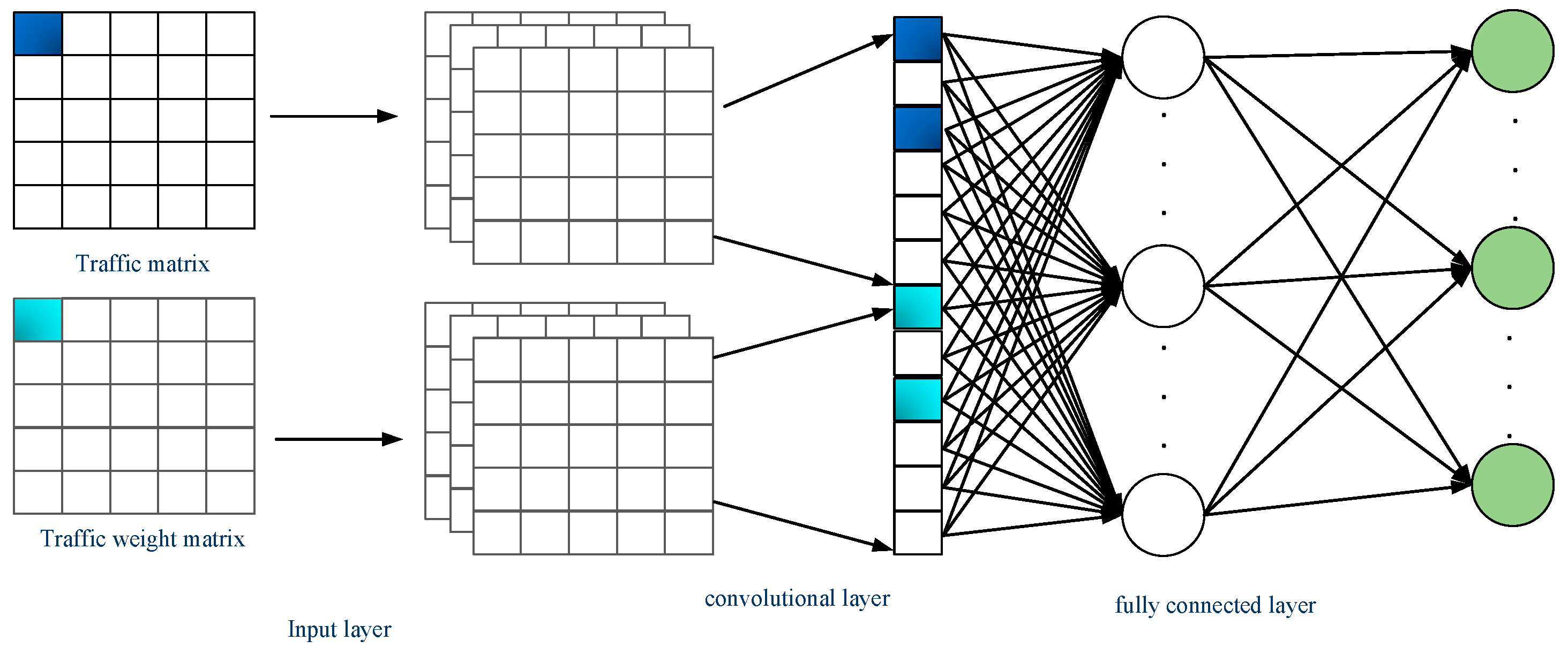
2.2. State and Action Space

1.
Input/State Space
The state space is represented by the following formula:
{ S = { S 1 , S 2 , , S t , , S n } S t = T M t T W t
where S t represents the state at time t , and T M t is the traffic matrix at time t , to express the bandwidth requirements among different data flows, indicating how much bandwidth each data flow needs for transmission. T W t is the data-flow weight matrix at time t , used to represent the weights of different categories of traffic, measuring the negative impact of different categories of data flows on the network during rerouting. T M t and T W t are isomorphic, with the only difference being the meanings of their elements, as indicated in Equation (2).
T = [ T 11 T 12 T 1 j T 1 n 2 T 21 T 22 T 2 j T 2 n 2     T i 1 T i 2 T i j T i n 2   T m 1 T m 2 T m j T m n 2 ]
In this context, n signifies the total count of nodes, while m corresponds to the number of time steps involved.
Data-flow weight values represent the proportion of network service traffic demanded by users within a data flow. A larger weight value indicates a higher demand for network service traffic by users. This definition is chosen to enhance the speed of network scheduling. The algorithm does not schedule each small network service individually but rather schedules each large data flow as a whole. Each large data flow comprises both user-demand network services and data center-demand network services. Data-flow weight values are used to distinguish their importance.
2.
Action Space
The action space can be represented by Equation (3).
A t = { 0 , 1 , , ( N × ( N 1 ) 1 ) }
For each state S t , CFRW-RL selects K critical flows. In a network system with N switch nodes, considering the source-destination switch perspective, a total of N × ( N 1 ) data flows exist, meaning that any switch acting as the source node can establish data flows with all other switches acting as destination nodes. Therefore, the action space contains all possible combinations of data flows, totaling C N × ( N 1 ) K combinations, where C N × ( N 1 ) K denotes the number of combinations of choosing K data flows from N × ( N 1 ) flows. The action space has a large scale, and directly computing all possible combinations would result in excessively high computational complexity. To reduce time complexity, CFRW-RL employs the method proposed by Zhang et al. [14] and Mao et al. [18], directly selecting K data flows from N × ( N 1 ) flows and associating each possible action with a specific data flow. This definition effectively reduces the scale of the action space, making the algorithm more efficient in addressing data-flow scheduling and rerouting problems.
During the algorithm’s iteration process, at each time step, K different data flows are chosen as the actions the agent will take in the next state:
a t K = { a t 1 , a t 2 , , a t K } .
This action-selection method ensures the algorithm’s rationality while reducing computational complexity, enabling CFRW-RL to better adapt to large-scale network systems and improve the efficiency of data-flow scheduling and rerouting.

2.3. Reward Function

The reward function is
r t = 1 U t ε * w f i K ( f i F K ) .
where U t represents the minimized maximum link bandwidth occupancy rate after optimization of key flow rerouting, F K = { f 1 , f 2 , , f i , , f K } represents the set of K critical flows, w f i represents the weight of the i-th critical f , ε represents the weight factor of critical flows in the reward function, and K is the number of critical flows. The term 1 / U t in the reward function translates the effect of optimizing and reducing the maximum link bandwidth occupancy rate, where a higher value results in a higher reward. The term ε * ( w f i / K ) represents the average weight of the selected K critical flows, where a smaller value leads to a higher reward. This is intended to encourage the algorithm to choose critical flows with a smaller impact on the network, thereby minimizing business interference.

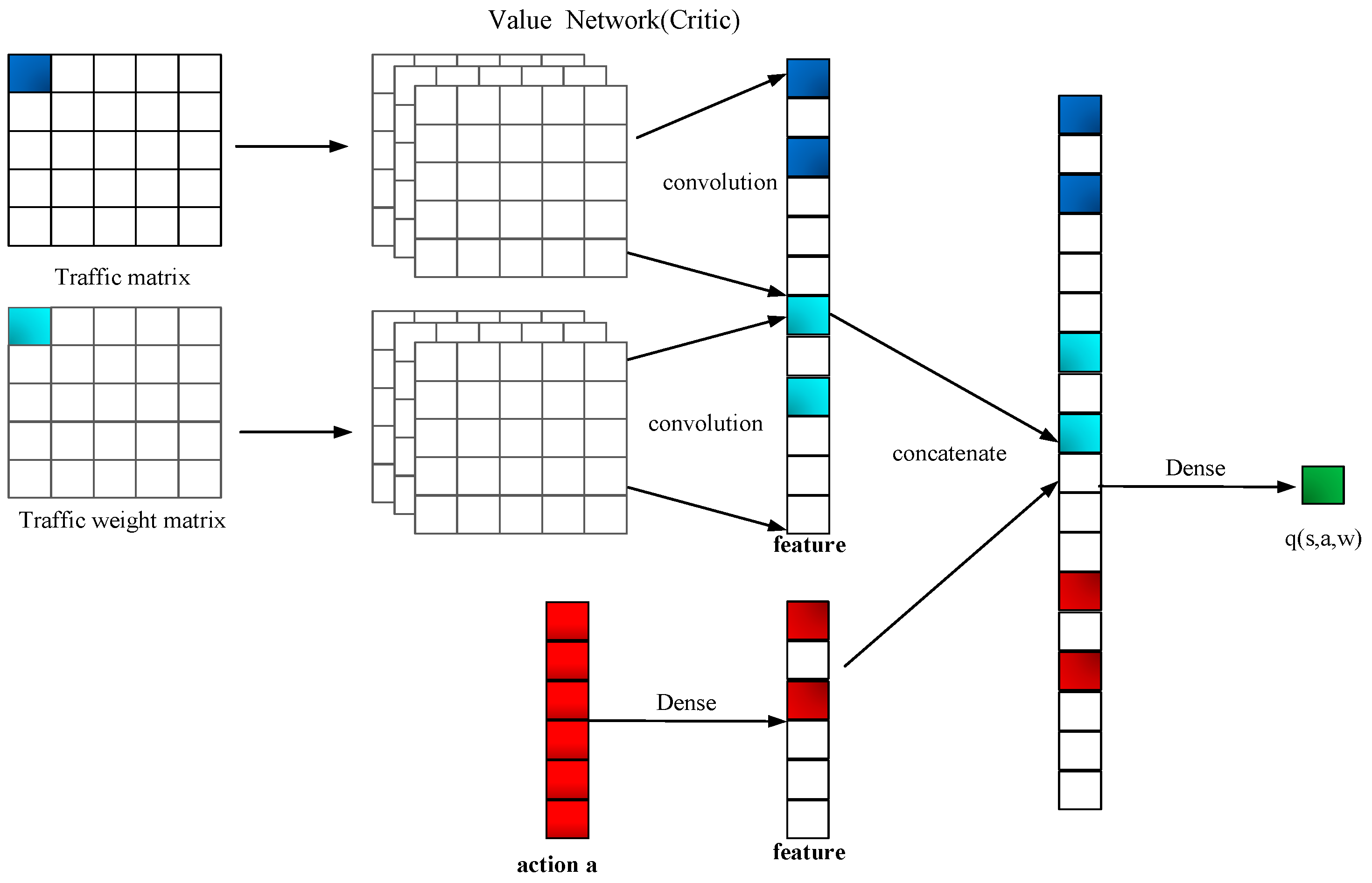
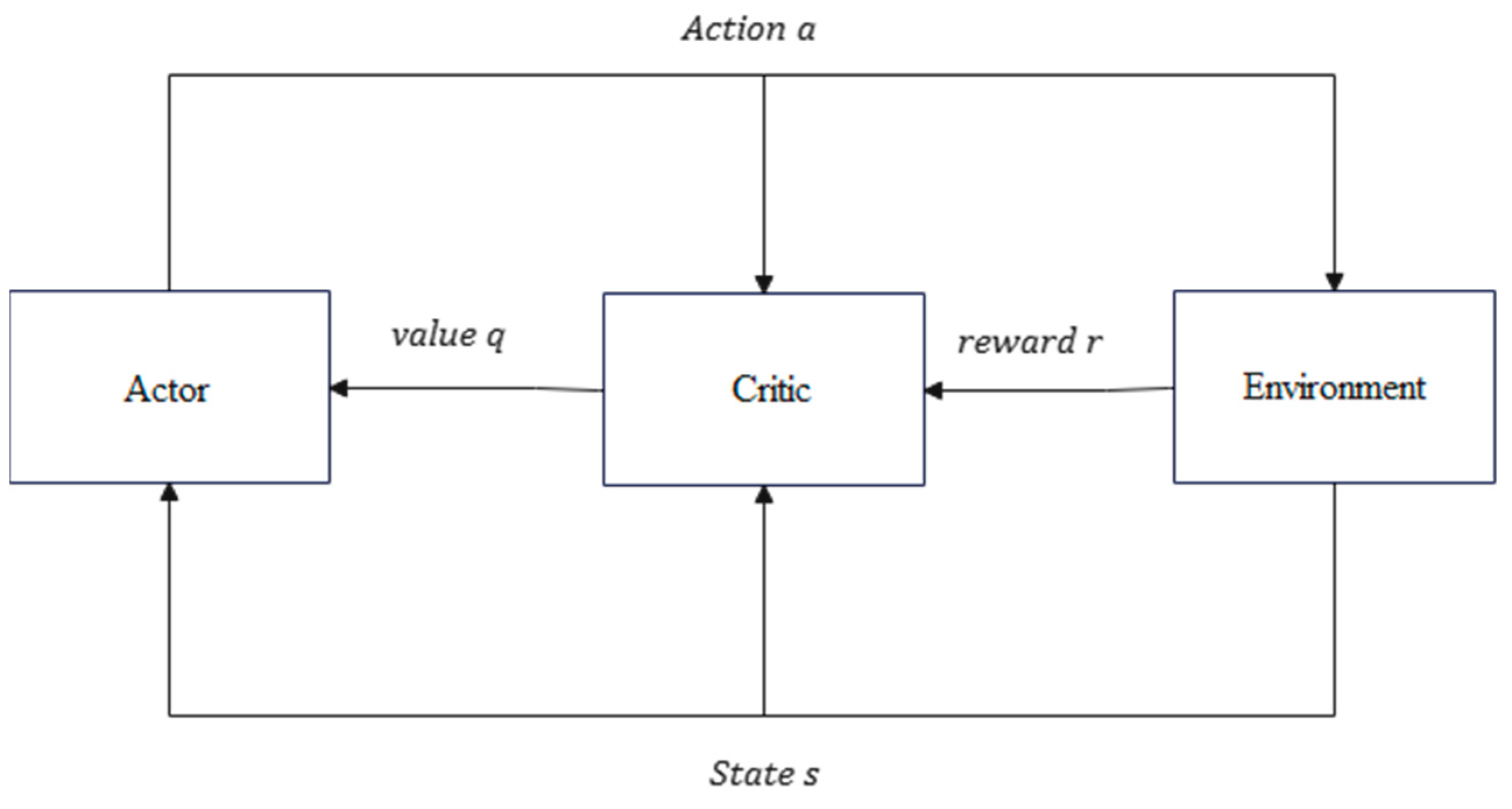
2.4. Actor Network and Critic Network

The CFRW-RL model utilizes a combined Actor–Critic architecture, where the Actor network is responsible for selecting actions based on a learned policy function. This policy function maps states to action probabilities, allowing for both the exploration of new strategies and the exploitation of known effective actions. The Critic network, on the other hand, estimates the value function, which predicts the expected cumulative reward for a given state or state–action pair. The Critic’s valuations provide feedback to the Actor, guiding it toward optimal policies that enhance network performance. The policy network and the value network’s structural diagrams are depicted in Figure 1 and Figure 2, respectively.
As illustrated in Figure 3, the model structure of the Actor–Critic method is presented.
The Actor is the policy network, responsible for generating actions, that is, selecting an action to perform in a given state. The Actor is typically parameterized by a policy function, which can be either deterministic or stochastic. The goal of the Actor is to optimize its policy through learning so as to achieve the maximum cumulative reward in the long term. The Critic, on the other hand, is the value network, responsible for evaluating the effectiveness of the actions taken by the Actor. It learns a value function to estimate the expected return of taking a specific action in a particular state. This value function can be either a state-value function or an action-value function, providing feedback to the Actor about the quality of its actions.
The state-value function of the Actor–Critic is defined as Equation (6):
V ( s ; θ , w ) = a π ( a | s ) q ( s , a ; w ) .
The equation represents the approximation of the state-value function using neural networks:
  • V ( s ; θ , w ) : this is the value function for state s , where θ represents the parameters of the policy network (Actor) and w represents the parameters of the value function network (Critic);
  • Σ a : this denotes the summation over all possible actions a , indicating the summation over the action space;
  • q ( s , a ; w ) : this is the State-action Value Function (Q-value Function) generated by the value function network, representing the expected value of taking action a in state s ;
  • π ( a | s ) : this is the action probability generated by the policy network, representing the probability of taking action. This is the action probability generated by the policy network, representing the probability of taking action a in state s .
In essence, this equation approximates the state-value function V ( s ; θ , w ) as a weighted sum of the state–action-value function q ( s , a ; w ) for all possible actions in state s , weighted by the corresponding action probabilities π ( a | s ) generated by the policy network.

3. The CFRW-RL Algorithm

This section elaborates on the CFRW-RL algorithm, focusing on the critical flow selection and rerouting processes that are central to its tTE approach.

3.1. Critical Flow Identification

The steps for updating the policy and value networks in the Actor–Critic method are as follows:
  • Observe the current state of the environment at time step t, use it as input, and calculate the probability distribution with the policy network. Randomly sample an action a t based on the computed probabilities.
  • The intelligent agent executes the action a t , the environment transitions to a new state s t + 1 , and a reward r t is given.
  • Use the new stat s t + 1 as input and calculate the probability distribution with the policy network. Randomly sample an action a t + 1 (note that this action is for computing the Q-value and is not actually executed).
  • Evaluate the value network using Equations (7) and (8).
    q t = q ( S t , a t , w t )
    q t + 1 = q ( S t + 1 , a ˜ t + 1 , w t )
  • Calculate the Temporal Difference (TD) error using Equation (9).
    δ t = q t ( r t + γ q t + 1 )
  • Derive the value network using Equation (10).
    d w , t = q ( s t , a t ; w ) w | w = w t
  • Update the value network using Equation (11). This involves gradient descent to make the predicted value closer to the TD target.
    w t + 1 = w t α δ t d w , t
  • Derive the policy network using Equation (12).
    d θ , t = log π ( a t | S t , θ ) θ | θ = θ t
  • Update the policy network using Equation (13). This involves gradient ascent to increase the score of the Actor’s action.
    θ t + 1 = θ t + β q t d θ , t
Each iteration of the Actor–Critic method requires the above nine steps, during which only one action is taken, one reward is observed, and the parameters of the neural network are updated once.
The pseudocode for the critical selection algorithm is shown in Algorithm 1.
Algorithm 1: pseudocode for the critical flow selection algorithm
1Initialize actor network parameters θ_actor, critic network parameters θ_critic
2Initialize actor optimizer optimizer_actor and critic optimizer optimizer_critic
3for each training iteration do:
4  Collect a batch of inputs, actions, rewards (and possibly next states) from the environment
5  with tf.GradientTape(tape1) as tape1:
6    Compute critic model’s value predictions values from inputs
7    Calculate value loss and advantages using value_loss_fn with rewards and values
8  Compute gradients for the critic network with tape1
9  Update critic network parameters using optimizer_critic and critic_gradients
10  with tf.GradientTape(tape2) as tape2:
11    Compute actor model’s policy logits from inputs
12    Calculate policy loss and entropy using policy_loss_fn with logits, actions, advantages, and entropy_weight
13  Compute gradients for the actor network with tape2
14  Update actor network parameters using optimizer_actor and actor_gradients
15End for
In this pseudocode:
  • ‘θ_actor’ and ‘θ_critic’ represent the parameters of the Actor network and Critic network, respectively.
  • ‘optimizer_actor’ and ‘optimizer_critic’ are the optimizers used to update the network parameters.
  • During each training iteration, a batch of inputs, actions, and rewards (and possibly next states) is first collected from the environment.
  • ‘tf.GradientTape’ is used to track the gradients of the Critic network, and to calculate the value loss and advantage values.
  • The gradients computed are used to update the parameters of the Critic network.
  • ‘tf.GradientTape’ is used again to track the gradients of the Actor network, and to calculate the policy loss and entropy.
  • The gradients computed are used to update the parameters of the Actor network.
This process is repeated over multiple training iterations until the network parameters converge to a point that optimizes the policy performance.

3.2. Critical Flow Rerouting Strategy

The traffic in the network consists of two parts: the critical flows that need to be rerouted and the residual flows outside the critical flows. Under the routing optimization strategy used in this paper, the residual flows are routed by default using the ECMP algorithm, while the critical flows are rerouted using linear programming. To minimize the maximum link utilization ratio in the network, we employed a linear programming (LP) model. A description of the symbols used in the model and their meanings are provided in Table 1.
If there are L links, with the load (i.e., traffic) on each link being l 1 , l 2 , , l L , and the capacity of each link being C 1 , C 2 , , C L , then the maximum utilization can be expressed as
U = max i = 1 L ( l i C i )
Here, l i / C i represents the utilization of the i -th link, which is the ratio of the traffic l i to the link capacity C i . By taking the maximum of the utilization ratios across all links, the maximum utilization rate of the entire network is obtained.
The model’s objective function is outlined in Equation (15), while the constraints are detailed in Equations (16)–(22).
o b j = minimize   U
d ( i ) + = k : < k , i > E p i , k s , d
d ( i ) = k : < i , k > E p k , i s , d
l i , j = < s , d > f E C M P p i , j s , d D s , d
l i , j f K = < s , d > f K p i , j s , d D s , d
l i , j = l i , j + l i , j f K ( < i , j > E , i V , j V )
l i , j C i , j U
d ( i ) + d ( i ) = { 1 i = = s 0 o t h e r 1 i = = d
The in-degree d ( i ) + and out-degree d ( i ) can be calculated as shown in Equations (15) and (16), respectively. The in-degree accounts for the sum of probabilities of traffic flow incoming to the node from others, whereas the out-degree corresponds to the sum of probabilities of traffic flow outgoing from the node to other nodes.
The initial load of the link < i , j > , representing the residual traffic assigned by the ECMP algorithm minus the critical flows’ traffic, is derived from Equation (17). The load of critical flows on the link < i , j > , as allocated by the key flow routing algorithm, is meticulously calculated using the model provided by Equation (18). This equation is pivotal in determining the portion of traffic that is deemed critical and how it is distributed across the network’s links. The total load on the link < i , j > , encompassing both the initial load and the critical flow load, is synthesized in Equation (19).
To ensure that link traffic remains within acceptable limits, the condition set forth in Equation (20) mandates that the total load on a link must be less than or equal to the product of its physical bandwidth and the maximum utilization rate. This constraint is crucial for preventing any link from being overloaded beyond its capacity.
Adhering to the principle of traffic conservation, data flows within the network are governed by a set of rules. These rules, as articulated in Equation (21), dictate the flow dynamics at various nodes. At the origin of a path, a node’s in-degree is null and its out-degree is one, resulting in a net difference of −1. Conversely, at the path’s terminus, the in-degree is one and the out-degree is zero, leading to a net difference of 1. For nodes that serve as intermediaries along the path, both the in-degree and out-degree are one, with no net difference between them.

4. Simulation and Results Analysis

4.1. Experimental Setup

4.1.1. Dataset

In this study, we utilize the Abilene open dataset, which was collected by Zhang [19], describing traffic information between core nodes of the Abilene network (the U.S. Education Network). The network topology consists of 12 network nodes and 30 links. This dataset records the traffic matrices between each pair of nodes in the network, with each traffic matrix size being 12 × 12. Traffic matrices are collected every 5 min, resulting in a total of 288 traffic matrices per day. The dataset spans 6 months, comprising 51,840 traffic matrices.

4.1.2. Evaluation Metrics

1.
Load-balancing Performance Ratio
To evaluate the load-balancing performance of the proposed CFRW_RL algorithm, we use the load-balancing performance ratio (P) as a metric. The calculation of the load-balancing performance ratio P is
P = U o p t U C F R W ,
where U o p t represents the optimized minimum maximum link bandwidth occupancy achieved through linear programming-based route optimization when the critical flow selection ratio is 100%. U C F R W is the minimized maximum link bandwidth occupancy obtained after selecting critical data flows based on the given critical flow selection ratio and optimizing their routing. A higher P value indicates better routing optimization effectiveness.
2.
Rerouting Disruption (RD)
RD is evaluated as the weighted average of the selected critical flows’ weights, calculated as
R D = ε w f i K ( f i F K ) ,
where K represents the number of critical flows, F K denotes the set of critical flows, fi represents the i-th critical flow, and w f i represents the weight of the i-th critical flow.
3.
Comparison Algorithms
To validate the effectiveness of the CFRW-RL algorithm, we employ three different methods for critical flow selection. Two rule-based heuristic algorithms are used: Top-K algorithm and Top-K critical algorithm. Additionally, a reinforcement learning-based algorithm is employed.
(1)
Top-K Algorithm
Selects the K flows with the highest traffic from the traffic matrix. The basic idea is that flows with higher traffic have a more significant impact on network performance.
(2)
Top-K Critical Algorithm
Selects the K flows with the highest traffic from the most congested links. The motivation is that flows passing through the most congested links have a larger impact on the network.
(3)
CFR-RL Algorithm
CFR-RL algorithm is a reinforcement learning-based TE solution. It dynamically adjusts routes based on network state and traffic demand by autonomously learning policies for selecting critical flows. It leverages the flexibility of software-defined networking (SDN).

4.2. Experiments and Results Analysis

4.2.1. Generation of Data-Flow Weight Values

To ensure the reasonability of data-flow weight values, we assume a similar distribution for the network service traffic demanded by users and the sizes of data flow traffic. Drawing inspiration from the distribution patterns of data center network service sizes studied in previous work [20] this study randomly selects some traffic matrices from the Abilene dataset. Common probability distributions are used to fit the traffic distribution patterns of each traffic matrix, and the goodness of fit for each probability distribution is calculated. The distribution with the highest fit is selected to generate data-flow weight values.
1.
Data Fitting
The specific steps for data fitting in this study are as follows. In the Abilene dataset, 1000 traffic matrices are randomly selected. Each traffic matrix is treated as an array, and the fitter toolkit is used to fit the distribution patterns of data items within each array. Fifteen common distribution patterns are used for data fitting, including norm, t, laplace, erlang, chi2, expon, exponpow, gamma, lognorm, uniform, pareto, weibull_min, weibull_max, exponweib, and dweibull. The distribution with the highest goodness of fit is selected, and the proportions of occurrence for these distributions are calculated. To ensure accuracy, we repeat the data-fitting process 10 times, and the average of the results is taken. Table 2 illustrates the fitted distribution patterns for data-flow weight values. The top four distribution patterns with the highest fit probability are exponweib, weibull_min, gamma, and lognorm.
2.
Generating Weights Based on Probability Distribution and Normalization
Drawing upon the findings presented in Table 2, this study opts for the “exponweib” probability distribution to assign weights to the traffic matrices in both the training and testing datasets. Subsequently, these weights are normalized to facilitate the training and evaluation of the CFRW-RL algorithm.

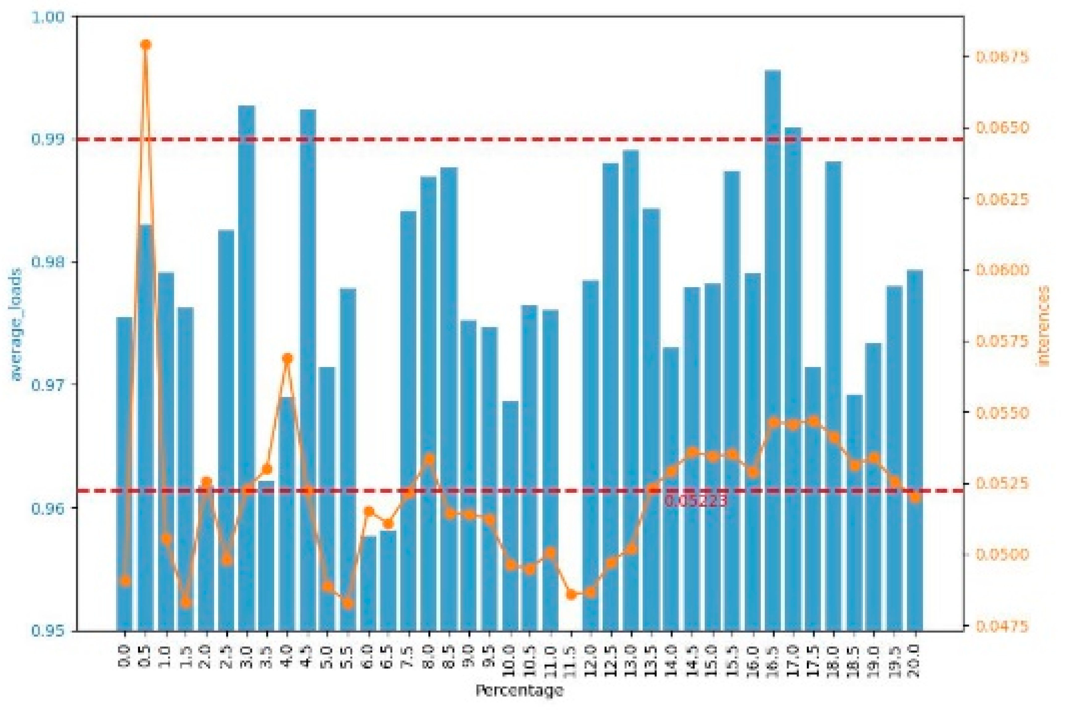
4.2.2. Impact of Key Flow Setting Ratio on CFRW-RL Algorithm

This section aims to explore the performance and effectiveness differences of the CFRW-RL algorithm under different critical flow selection ratios. To achieve this, we conduct a series of simulation experiments on the Abilene dataset. We divide the critical flow selection ratio from 0 to 30% into 16 groups uniformly, where 0% represents the default ECMP algorithm. We randomly select 2500 traffic matrices as experimental data, with 2000 used for training the CFRW-RL model and 500 for testing the CFRW-RL algorithm. The network load-balancing performance ratio under different critical flow ratios is calculated using (12), and histograms are generated, as shown in Figure 1.
As depicted in Figure 4, the left y-axis corresponds to the load-balancing ratio, while the right y-axis indicates the average weight of the selected critical flows. Observations from Figure 4 reveal that across load ratios of 10, 12, 14, 16, 18, and 20%, the load-balancing ratios consistently surpass 97%. The primary objective of the CFRW-RL algorithm is to reduce the average weight of the chosen critical flows, thereby mitigating business interference. Among the six examined key flow ratios, the minimum average weight of the selected critical flows is achieved at a key flow ratio of 10%. Consequently, for the subsequent experiments, a key flow ratio of 10% is maintained to optimize the trade-off between the load-balancing ratio and the rate of business interference.

4.2.3. Effect of Weight Proportion ε on CFRW-RL Algorithm

During the analysis of the CFRW-RL algorithm’s impact on weight distribution, we fixed the proportion of critical flows at 10%, and varied the weight ratio ε from 0 to 20, incrementing by 0.5 for each step. For each distinct value of ε, we documented the load ratio and the average reward value, as illustrated in Figure 5. A weight value of 0 signifies the absence of the traffic weight matrix’s application, which implies that the CFR-RL algorithm is not being utilized.
The load-balancing ratio and the average weight of the selected critical flows are delineated in Figure 5, with the former indicated by the left vertical axis and the latter by the right vertical axis. Notably, the load-balancing ratio achieves a figure above 99% at weight coefficients of 3.0, 4.5, 16.5, and 17.0. The CFRW-RL algorithm’s primary goal is to optimize the balance between maintaining a high load-balancing ratio and minimizing the average weight of critical flows. Among the coefficients tested, the lowest average weight is observed at a coefficient of 4.5, signifying an optimal configuration for balancing load and reducing flow weights. In light of these findings, a weight coefficient of 4.5 is selected for implementation in subsequent experimental trials.

4.2.4. Validation of the Effectiveness of a Reinforcement Learning Network Structure

The convolutional layers in the policy network are utilized to extract features related to the weights of data flows. To investigate the performance of the CFRW-RL algorithm under different policy network architectures, we vary the number of convolutional kernels, setting them to 64, 128, and 256, respectively. Three sets of experiments are conducted using the Abilene dataset, comparing the three network structures based on indicators such as the load-balancing ratio, algorithm optimization time, and business interference rate. The comparison of business interference rates for different network structures with CFRW-RL is shown in Figure 6.
From the results presented in Figure 5, it is evident that an increase in the number of nodes leads to a corresponding increase in the optimization time required by the algorithm. This is attributable to the fact that a higher node count demands greater learning time and computational resources. Moreover, when the number of nodes in the convolutional layer is set to 128, the algorithm achieves the optimal balance, with the highest load-balancing ratio and the lowest business disturbance rate. Consequently, this study has opted for a configuration of 128 nodes.
It is important to note that having too few nodes can result in insufficient learning capacity for the policy network, while an excessive number of nodes can lead to an increased business disturbance rate. This is primarily due to the risk of overfitting in the policy network, which can compromise the robustness of the algorithm. Additionally, as the size of the policy network grows, so does the time required to train the model. Therefore, selecting an appropriate network size is crucial for effectively balancing algorithm performance and training duration.

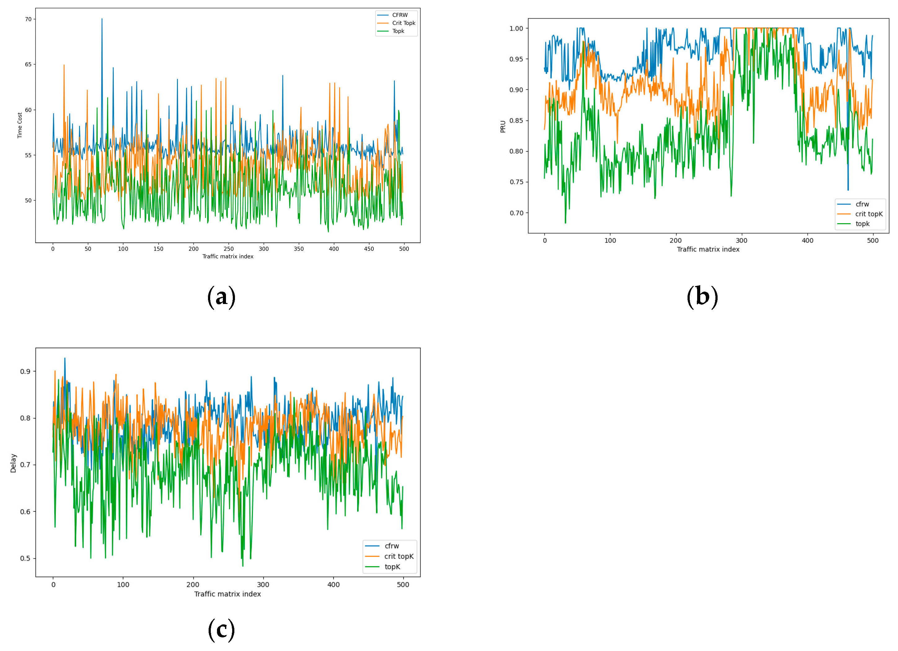
4.2.5. Performance Comparison between CFRW-RL Algorithm and Heuristic Algorithms

The comparison between the CFRW-RL algorithm and heuristic algorithms Crit_TopK and TopK in terms of the optimization time, load-balancing ratio, and delay is illustrated in Figure 7a–c.
As depicted in Figure 7, the CFRW-RL algorithm shows a modest increase in optimization time and delay when compared with the heuristic algorithms, namely top K and crit-topK. Despite this, the CFRW-RL algorithm significantly outperforms these two heuristic algorithms in terms of load-balancing ratio. This distinction is particularly crucial in scenarios that demand high real-time responsiveness, with video applications being a prime example.
The slight increase in optimization time and delay for the CFRW-RL algorithm can be attributed to its more sophisticated approach to learning and adapting to network conditions. The algorithm’s reinforcement learning framework involves a continuous process of evaluating and adjusting its strategy to achieve better long-term performance, which inherently requires more computational effort and time compared to heuristic algorithms that follow simpler, rule-based procedures.
However, the superior load-balancing ratio achieved by the CFRW-RL algorithm justifies the additional computational overhead. A higher load-balancing ratio ensures that network resources are utilized more efficiently, leading to a more stable and reliable network performance, which is essential for maintaining the quality of service (QoS) for real-time applications, such as video streaming or video conferencing.

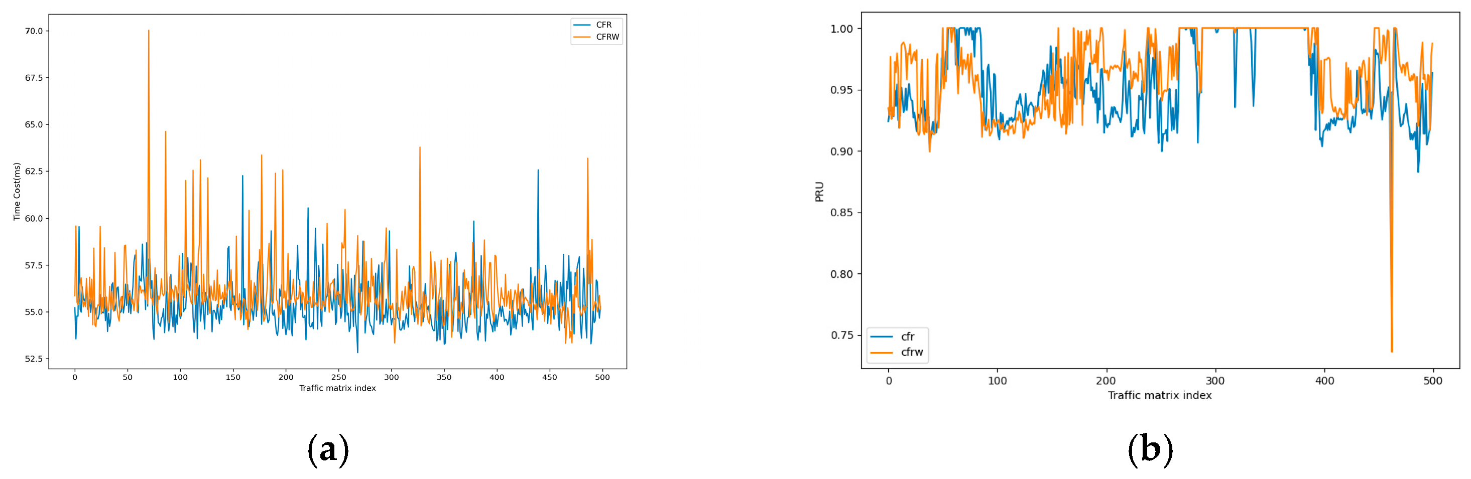
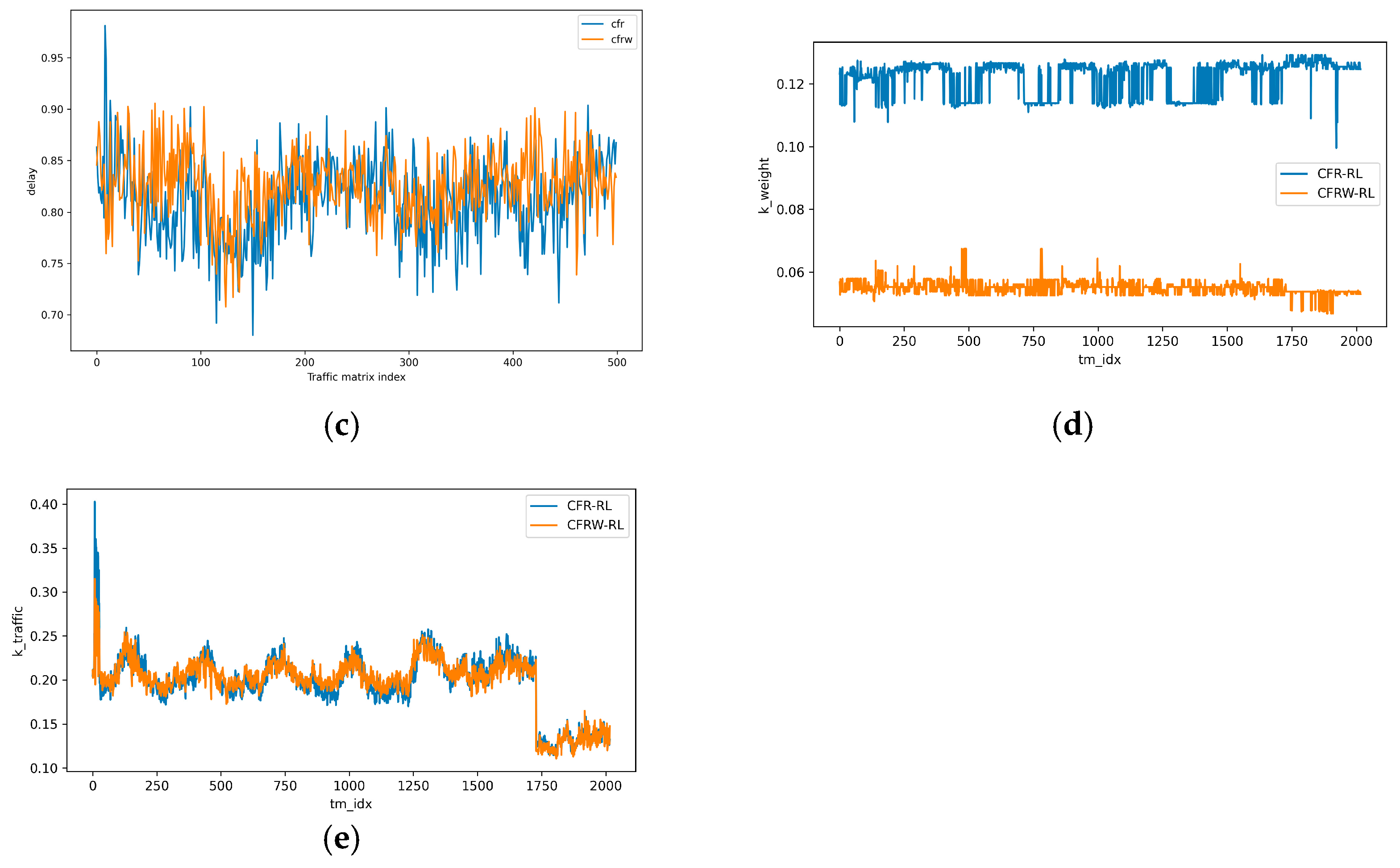
4.2.6. Performance Comparison between the CFRW-RL Algorithm and CFR-RL Algorithm

The comparison results of CFRW-RL and CFR-RL algorithms in terms of optimization time consumption, load-balancing ratio, and delay are shown in Figure 8a–c, respectively. The business interference rate is calculated in two ways: the first one is based on the calculation of the business interference rate in the CFR-RL algorithm, which computes the ratio of the traffic of critical flows to the total traffic; the second one is based on the calculation of the business interference proportion in the CFRW-RL algorithm, which calculates the average weight of the selected critical flows. The comparisons of the two business interference rates of the algorithm are shown in Figure 8d,e.
As depicted in Table 3, the comparison of CFRW-RL and CFR-RL algorithms across various key performance indicators such as time consumption, load balancing, delay, average traffic of critical flows, and average weight of critical flows is presented. This table provides a detailed comparative analysis, allowing for a better understanding of the strengths and suitable applications of each algorithm.
The results presented in Figure 8, along with the data from Table 2, indicate that the CFRW-RL algorithm has a marginal improvement in time consumption compared to the CFR-RL algorithm, with a reduction of 0.6 s. This slight decrease suggests a potential for increased efficiency in the CFRW-RL algorithm. Both algorithms exhibit a high load-balancing ratio, exceeding 95%, which is indicative of their effectiveness in distributing network traffic evenly and preventing potential bottlenecks.
One of the most notable differences between the two algorithms is observed in their handling of critical flows. The CFRW-RL algorithm selects critical flows with an average traffic rate that is almost identical to that of the CFR-RL algorithm. However, the CFRW-RL algorithm achieves this with a significantly lower average weight of critical flows, which is more than 67% less than that of the CFR-RL algorithm. This lower average weight implies that the CFRW-RL algorithm introduces less interference with business operations, which is a crucial factor in maintaining the smooth functioning of business applications.
The CFRW-RL algorithm accomplishes this through its reward computation mechanism, which deducts the average weight of critical flows from the rewards calculated by the CFR-RL algorithm. By doing so, the CFRW-RL algorithm incentivizes the selection of critical flows with lower average weights, as lower average weights result in higher rewards. This approach not only reduces business interference but also enhances the overall efficiency of network traffic management.
The significant reduction in business interference, as highlighted by the lower average weight of critical flows, underscores the effectiveness of the CFRW-RL algorithm in mitigating disruptions to business operations. This improvement is particularly important in scenarios where network performance directly impacts business outcomes, as it ensures that critical business applications run smoothly without unnecessary delays or interference.
In conclusion, the CFRW-RL algorithm, as demonstrated by the data in Table 2 and the visualization in Figure 8, offers a refined approach to network traffic management. It successfully balances the reduction of time consumption and load balancing with the minimization of business interference, making it a potentially superior choice for environments that require high performance and minimal disruption to business operations.

5. Conclusions

In the domain of backbone link traffic scheduling within enterprise networks, the aim to minimize the disruption to business activities during the process of traffic scheduling has led to the introduction of data-flow weights in this study. We propose an enhanced learning algorithm that leverages these weights, known as CFRW-RL. This algorithm is an extension of the CFR-RL algorithm and integrates a traffic-weight matrix. This integration enables the algorithm to automatically identify and prioritize critical flows that are associated with lower business interference for rerouting. This approach facilitates more intelligent and precise traffic scheduling, ensuring that the network’s performance is optimized with minimal impact on business processes.
The simulation experiments conducted to evaluate the performance of CFRW-RL have demonstrated its superiority over the CFR-RL algorithm. The findings reveal that the CFRW-RL algorithm is capable of achieving near-optimal performance by rerouting only a small fraction of the total traffic. This strategic rerouting significantly reduces the interference typically caused by traffic scheduling adjustments on business operations. By focusing on the average traffic of critical flows and their associated weights, CFRW-RL effectively balances network efficiency with the operational needs of the enterprise, leading to a more streamlined and business-friendly network environment.
In future work, we aim to focus on the following areas for research and improvement:
  • Adaptive Weight Adjustment Mechanism: We will research and develop a mechanism that can dynamically adjust the weights of data flows based on real-time network conditions and business requirements. This will help achieve more refined and effective traffic management in changing network environments.
  • Algorithmic Scalability: We will investigate the scalability of the algorithm for large enterprise networks, particularly in the face of complex network topologies and high volumes of traffic, to ensure the effectiveness and efficiency of the algorithm.
  • Real-World Deployment and Testing: We plan to deploy and test the CFRW-RL algorithm in real enterprise network environments to verify its practical applicability and to further optimize the algorithm’s performance based on actual data.

Author Contributions

Conceptualization, H.C. and L.Z.; methodology, H.C. and Y.L.; software, H.C. and Y.L.; validation, Z.L.; formal analysis, H.C.; data curation, Y.L.; writing—original draft preparation, H.C.; writing—review and editing, L.Z.; visualization, Z.L.; supervision, L.Z.; project administration, H.C. All authors have read and agreed to the published version of the manuscript.

Funding

This research was funded by Guangdong Province’s Special Fund for Science and Technology Innovation Strategy, grant number pdjh2023b0986; Guangdong Vocational and Technical Education Association’s Fourth Council Research Planning Project, grant number 202212G266; Zhuhai City Polytechnic scientific research projects, grant number KY2022Z01Z; and Zhuhai Education Research Planning Project, grant number 2023ZHGHKT261.

Data Availability Statement

Data are available in a publicly accessible repository that does not issue DOIs. Publicly available datasets were analyzed in this study. This data can be found here: [https://www.cs.utexas.edu/~yzhang/research/AbileneTM (accessed on 8 April 2024)].

Conflicts of Interest

The authors declare no conflicts of interest.

References

  1. Garani, S.S.; Zhang, T.; Motwani, R.H.; Pozidis, H.; Vasic, B. Guest Editorial Channel Modeling, Coding and Signal Processing for Novel Physical Memory Devices and Systems. IEEE J. Sel. Areas Commun. 2016, 34, 2289–2293. [Google Scholar] [CrossRef]
  2. Chang, H.; Kodialam, M.; Lakshman, T.V.; Mukherjee, S.; Van der Merwe, J.K.; Zaheer, Z. MAGNet: Machine Learning Guided Application-Aware Networking for Data Centers. IEEE Trans. Cloud Comput. 2023, 11, 291–307. [Google Scholar] [CrossRef]
  3. Garcia-Dorado, J.L.; Rao, S.G. Cost-aware Multi Data-Center Bulk Transfers in the Cloud from a Customer-Side Perspective. IEEE Trans. Cloud Comput. 2019, 7, 34–47. [Google Scholar] [CrossRef]
  4. Zhu, J.; Jiang, X.; Yu, Y.; Jin, G.; Chen, H.; Li, X.; Qu, L. An efficient priority-driven congestion control algorithm for data center networks. China Commun. 2020, 17, 37–50. [Google Scholar] [CrossRef]
  5. Islam, S.U.; Javaid, N.; Pierson, J.M. A novel utilisation-aware energy consumption model for content distribution networks. Int. J. Web Grid Serv. 2017, 13, 290. [Google Scholar] [CrossRef]
  6. Guo, Y.; Ma, Y.; Luo, H.; Wu, J. Traffic Engineering in a Shared Inter-DC WAN via Deep Reinforcement Learning. IEEE Trans. Netw. Sci. Eng. 2022, 9, 2870–2881. [Google Scholar] [CrossRef]
  7. Xu, Z.; Tang, J.; Meng, J.; Zhang, W.; Wang, Y.; Liu, C.H.; Yang, D. Experience-driven Networking: A Deep Reinforcement Learning based Approach. In Proceedings of the IEEE INFOCOM 2018—IEEE Conference on Computer Communications, Honolulu, HI, USA, 16–19 April 2018; pp. 1871–1879. [Google Scholar]
  8. Guo, Y.; Wang, W.; Zhang, H.; Guo, W.; Wang, Z.; Tian, Y.; Yin, X.; Wu, J. Traffic Engineering in Hybrid Software Defined Network via Reinforcement Learning. J. Netw. Comput. Appl. 2021, 189, 103116. [Google Scholar] [CrossRef]
  9. Sun, P.; Hu, Y.; Lan, J.; Tian, L.; Chen, M. TIDE: Time-relevant deep reinforcement learning for routing optimization. Future Gener. Comput. Syst. 2019, 99, 401–409. [Google Scholar] [CrossRef]
  10. Sun, P.; Guo, Z.; Lan, J.; Li, J.; Hu, Y.; Baker, T. ScaleDRL: A Scalable Deep Reinforcement Learning Approach for Traffic Engineering in SDN with Pinning Control. Comput. Netw. 2021, 190, 107891. [Google Scholar] [CrossRef]
  11. Rischke, J.; Sossalla, P.; Salah, H.; Fitzek, F.H.P.; Reisslein, M. QR-SDN: Towards Reinforcement Learning States, Actions, and Rewards for Direct Flow Routing in Software-Defined Networks. IEEE Access 2020, 8, 174773–174791. [Google Scholar] [CrossRef]
  12. Wu, T.; Zhou, P.; Wang, B.; Li, A.; Tang, X.; Xu, Z.; Chen, K.; Ding, X. Joint traffic control and multichannel reassignment for core backbone network in SDN-IoT: A multi-agent deep reinforcement learning approach. IEEE Trans. Netw. Sci. Eng. 2020, 8, 231–245. [Google Scholar] [CrossRef]
  13. Zhang, H.; Zhang, J.; Bai, W.; Chen, K.; Chowdhury, M. Resilient datacenter load balancing in the wild. In Proceedings of the Conference of the ACM Special Interest Group on Data Communication, Los Angeles, CA, USA, 21–25 August 2017; pp. 253–266. [Google Scholar]
  14. Zhang, J.; Ye, M.; Guo, Z.; Yen, C.-Y.; Chao, H.J. CFR-RL: Traffic Engineering with Reinforcement Learning in SDN. IEEE J. Sel. Areas Commun. 2020, 38, 2249–2259. [Google Scholar] [CrossRef]
  15. Wu, X.; Huang, C.; Tang, M.; Sang, Y.; Zhou, W.; Wang, T.; He, Y.; Cai, D.; Wang, H.; Zhang, M. NetO: Alibaba’s WAN Orchestra-tor[EB/OL]. 2017. Available online: http://conferences.sigcomm.org/sigcomm/2017/files/program-industrial-demos/sigcomm17industrialdemos-paper1.pdf (accessed on 26 October 2017).
  16. Wang, R.; Zhang, Y.; Wang, W.; Xu, K.; Cui, L. Algorithm of Mixed Traffic Scheduling Among Data Centers Based on Prediction. J. Comput. Res. Dev. 2021, 58, 1307–1317. [Google Scholar] [CrossRef]
  17. Kandula, S.; Menache, I.; Schwartz, R.; Babbula, S.R. Calendaring for wide area networks. In Proceedings of the 2014 ACM conference on SIGCOMM, Chicago, IL, USA, 17–22 August 2014; pp. 515–526. [Google Scholar]
  18. Mao, H.; Alizadeh, M.; Menache, I.; Kandula, S. Resource management with deep reinforcement learning. In Proceedings of the 15th ACM Workshop on Hot Topics in Networks, Atlanta, GA, USA, 9–10 November 2016; pp. 50–56. [Google Scholar]
  19. Zhang, Y. Abilene Network Traffic Data[EB/OL]. 2023. Available online: https://www.cs.utexas.edu/~yzhang/research/AbileneTM (accessed on 26 October 2017).
  20. Benson, T.; Akella, A.; Maltz, D.A. Network traffic characteristics of data centers in the wild. In Proceedings of the 10th ACM SIGCOMM Conference on Internet measurement, Melbourne, Australia, 1–3 November 2010; pp. 267–280. [Google Scholar]
Figure 1. Structural diagram of the policy network.
Electronics 13 01441 g001
Figure 2. Structural Diagram of the value network.
Electronics 13 01441 g002
Figure 3. The model structure of the Actor–Critic method.
Electronics 13 01441 g003
Figure 4. Influence of different critical flow ratios on link load ratios.
Electronics 13 01441 g004
Figure 5. The influence of traffic weight proportion on the CFRW-RL algorithm.
Electronics 13 01441 g005
Figure 6. This is a performance comparison of CFRW-RL algorithm for different numbers of convolutional layer nodes. (a) Comparison of description of load-balancing ratios for different numbers of nodes in convolutional layers; (b) comparison of algorithm optimization time for different numbers of nodes in convolutional layers; (c) comparison of business disruption rates for different numbers of nodes in convolutional layers.
Electronics 13 01441 g006
Figure 7. This is a performance comparison between CFRW-RL algorithm and heuristic algorithms. (a) Comparison of time consumption for optimization between CFRW-RL algorithm and heuristic algorithm; (b) comparison of load-balancing ratios between CFRW-RL algorithm and heuristic algorithm; (c) comparison of optimization latency between CFRW-RL algorithm and heuristic algorithm.
Electronics 13 01441 g007
Figure 8. This is a performance comparison between CFRW-RL and CFR-RL. (a) Comparison of time consumption for optimization between CFRW-RL and CFR-RL; (b) comparison of load-balancing ratios between CFRW-RL and CFR-RL; (c) comparison of optimization latency between CFRW-RL algorithm and CFR-RL c algorithm; (d) comparison of business interference rate (average weight of critical flows) between CFRW-RL and CFR-RL; (e) comparison of business interference rates (average traffic of critical flows) between CFRW-RL and CFR-RL.
Electronics 13 01441 g008aElectronics 13 01441 g008b
Table 1. Symbols and their meanings.
SymbolMeaning
C i , j The physical bandwidth of link < i , j > E , i V , j V .
l i , j The total load of link < i , j > , < i , j > E , i V , j V .
l i , j The initial load of link < i , j > E , i V , j V .
f K The set of K critical flows identified by the CFRW-RL algorithm.
f E C M P The residual flows excluding f K .
D s , d The bandwidth requirement for the data flow from source node s to destination node d, s V , d V , s d .
p i , j s , d The probability of the data flow from source node s to destination node d traversing link < i , j > , s V , d V , s d , < i , j > E .
UThe maximum bandwidth utilization across various links in the network.
D ( f E C M P ) The traffic demand employing the ECMP algorithm.
D ( f K ) The traffic demand of critical flow f K .
d ( i ) + The in-degree of node i
d ( i ) The out-degree of node i.
l i , j f K The traffic load of critical flow allocated to link < i , j > .
Table 2. Fitted distribution of data stream weights.
Probability DistributionEXPONWEIBWEIBULL_MINGammaGammaOther
Percentage43.95%20.19%17.7%12.81%5.35%
Table 3. Performance comparison between CFRW-RL and CFR-RL algorithms.
AlgorithmTime Consumption (ms)Load-Balancing RatioDelay
(ms)
The Average TrafficThe Average Weight
CFRW-RL56.0495.7%0.80750.19720.0550
CFR-RL55.4495.6%0.80680.19650.1673
Disclaimer/Publisher’s Note: The statements, opinions and data contained in all publications are solely those of the individual author(s) and contributor(s) and not of MDPI and/or the editor(s). MDPI and/or the editor(s) disclaim responsibility for any injury to people or property resulting from any ideas, methods, instructions or products referred to in the content.

