Concurrent Learning-Based Two-Stage Predefined-Time System Identification

Abstract

This paper proposes a novel two-stage predefined-time system identification algorithm for uncertain nonlinear systems based on concurrent learning. The main feature of the algorithm is that the convergence time of estimation error is an exact predefined parameter, which can be known and adjusted directly by users. Historic identification data are stored in the first stage to guarantee that a finite-rank condition is satisfied. In the second stage, the estimation error converges to zero for linearly parameterized uncertain systems, or it is regulated into the neighborhood of zero for unknown systems modeled by neural networks. The identification algorithm takes effect without the restrictive requirement of the persistent excitation condition. Simulation examples verify the effectiveness of the proposed method.

1. Introduction

System identification and parameter estimation for linear, nonlinear, and other kinds of systems are significant problems, since their solution always forms the basis of posterior control synthesis. The system identification issue has remained critical and difficult to solve in control theory, despite the variety of methods used to tackle and improve it [1].

For parameter estimations to converge to their true values, or close to a neighborhood of them, the regressors used in traditional online identification algorithms must be persistently exciting (PE) [2]. Nevertheless, it is hard to achieve the restrictive PE condition all the time [3]. In order to overcome this drawback, the concurrent learning (CL) method, proposed by [4,5], has drawn attention in the past decade. Historic data with online data are concurrently utilized in CL-based identification algorithms to achieve the convergence of estimation errors under relaxed finite-excitation conditions. Afterwards dynamic state-derivative estimator-based CL [6] and integral concurrent learning methods [7,8,9] were developed, removing the knowledge of state derivatives in the CL-based identification approaches [4,5].

The system identification rate always has an appreciable effect on control efficiency. Early CL-based system identification methods [4,5,6,7,8,9] guaranteed exponential convergence of parameter estimation errors. In recent years, several identification methods with limited estimation time have been investigated. Refs. [10,11,12,13,14] proposed finite-time parameter estimators for robotic systems. To remove the PE condition imposed on the algorithms in [10,11,12,13,14], Refs. [15,16] proposed CL-based finite-time system identification algorithms for unknown systems modeled by neural networks (NNs). However, the upper bounds of the settling time provided by finite-time identification methods [15,16] may increase with increases in the initial estimation error.

In order to guarantee the uniformity of the settling time boundary with the initial estimation error in an identification algorithm, Refs. [17,18] designed fixed-time system identification methods by using fixed-time Lyapunov dynamics. However, the settling times of estimation errors in [17,18] were formulated as complex expressions, which contain series of design parameters. Furthermore, the steady estimation error may not be exactly zero for the parameter estimation case [17], and the provided settling time function in the CL-based fixed-time identification algorithm in [18] may be uncertain since its formula contains unknown information about neural network approximation errors (NNAEs). Moreover, some fixed-time parameter identification algorithms have been studied based on the dynamic regressor extension and mixing (DREM) method. Ref. [19] added a shifting and scaling factor in the DREM-based parameter estimation law, and proved that the solution of the estimation error reaches zero in a fixed time. Then, Ref. [20] proposed a two-stage fixed-time DREM estimator with an integral time-varying gain. However, the fixed convergence time boundaries of estimation errors in [19,20] are determined by unknown times when the initial excitation of dynamic regressors is achieved, thus being unadjustable a priori by users from the viewpoint of practicality.

Recently, there has been a great deal of attention on the analysis of a class of systems known as predefined-time stable systems [21,22,23,24,25,26], since the settling time boundary of such systems is an exactly known design parameter. In the view of the advantage of predefined-time stability, predefined-time system identification should be also investigated for the sake of estimation time presetting. A predefined-time identification algorithm provides an exact time when the estimation of an unknown system is available for controllers. Several parameter estimation algorithms with the predefined-time property were studied based on prescribed performance control [27,28], where the convergence times of estimation errors are explicit design parameters in performance functions. The estimation errors in [27,28] can be restricted into arbitrary small regions, but they may not be eliminated entirely after the provided predefined times without considering modeling errors. Ref. [29] proposed a predefined-time DREM parameter estimator using predefined-time Lyapunov dynamics, but the provided convergence time boundary is affected by the unknown time when the dynamic regressor is excited to some certain value. It is hard to set the upper bound of convergence time with [29] without the prior excitation information of the dynamic regressor.

Motivated by the aforementioned, this paper aims to design a new CL-based identification algorithm for a class of uncertain systems, providing users with an explicit design parameter as the desired convergence time boundary without the PE condition. The whole identification process is divided into two stages. In the first stage, historic identification data are recorded until a finite-rank condition rather than the strict infinite PE condition is satisfied. In the second stage, the estimation error can converge to zero accurately without NNAEs, or it can be steered into the neighborhood of zero if NNAEs exist, within an explicit predefined time. The main contributions of the paper can be summarized as follows:

(1) The provided settling time boundary of the proposed identification algorithm is an explicit design parameter that can be known and adjusted directly by users. This predefined-time parameter is related to neither the unknown information about NNAEs compared with the traditional CL-based fixed-time algorithm [18], nor the unavailable information of initial excitation time compared with traditional DREM-based fixed-time or predefined-time identification algorithms [19,20,29].

(2) The identification accuracy is much improved theoretically. Compared with traditional fixed-time and predefined-time estimators [17,27,28], it is proven that the estimation error converges to zero exactly, rather than zero nearby, without NNAEs after the predefined settling time.

(3) The identification algorithm takes effect under an easier finite-rank condition rather than the restrictive infinite PE condition compared with traditional finite-time and fixed-time identification studies [11,12,13,14,27,28], enhancing the practicality of the proposed approach.

Notation 1.

In this paper, $\mathbb{R}$ is the set of real numbers, ${\mathbb{R}}^n$ is the set of n-dimensional real vectors, ${\mathbb{R}}^{m_1\times m_2}$ is the set of $m_1\times m_2$ real matrices, $0_n\in {\mathbb{R}}^n$ denotes an n-dimensional zero vector, $I_n\in {\mathbb{R}}^{n\times n}$ denotes an identity matrix, and $\mathrm{tr}(·)$ denotes the trace of a matrix $(·)$. For any vector $\alpha ={[{\alpha }_1,\cdots ,{\alpha }_n]}^T\in {\mathbb{R}}^n$, $\parallel \alpha \parallel$ is its Euclidean norm, ${\alpha }^T$ is its transpose vector, ${\lfloor {\alpha }^T\rceil }^{\gamma }=\left[\right|{\alpha }_1{|}^{\gamma }\mathrm{sign}\left({\alpha }_1\right),\cdots ,|{\alpha }_n{{|}^{\gamma }\mathrm{sign}\left({\alpha }_n\right)]}^T$, where $\mathrm{sign}(·)$ denotes the sign function of $(·)$ and $\gamma \in \mathbb{R}$ denotes a positive constant. For any $a_1,a_2,a_3\in \mathbb{R}$ with $a_3\ne 0$, $a_1\equiv a_2\left(\mathrm{mod}{a}_3\right)$ denotes that $(a_1-a_2)/a_3$ is an integer. For any matrix $Z_1\in {\mathbb{R}}^{m_1\times m_2}$, $\parallel Z_1\parallel$ denotes its Frobenius norm, and for any symmetric positive-definite (or semi-definite) matrix $Z_2\in {\mathbb{R}}^{m_1\times m_1}$, ${\lambda }_{min}\left(Z_2\right)$ and ${\lambda }_{max}\left(Z_2\right)$ denote its minimum eigenvalue and maximum eigenvalue, respectively.

2. Problem Formulation and Preliminaries

Consider the following uncertain nonlinear system:

$$\begin{array}{c}\hfill \dot{x}\left(t\right)=f\left(x\left(t\right)\right)+g\left(x\left(t\right)\right)u\left(t\right),x\left(0\right)=x_0\in \mathbb{R}\end{array}$$

(1)

where $x\in {\mathcal{D}}_x\subset {\mathbb{R}}^n$ is measurable system state, $u\in {\mathcal{D}}_u\subset {\mathbb{R}}^m$ is the control input, and ${\mathcal{D}}_x$ and ${\mathcal{D}}_u$ denote two known compact sets; $f:{\mathcal{D}}_x\to {\mathbb{R}}^n$ and $g:{\mathcal{D}}_x\to {\mathbb{R}}^{n\times m}$ represent unknown system drift dynamics and input dynamics, respectively, and they are locally Lipschitz in $x\left(t\right)$.

The unknown dynamics $f\left(x\right(t\left)\right)$ and $g\left(x\right(t\left)\right)$ may be modeled accurately as the linearly parameterized form [18]

$$\begin{array}{c}\hfill f\left(x\left(t\right)\right)={\theta }_f^{\ast T}{\xi }_f\left(x\left(t\right)\right),g\left(x\left(t\right)\right)={\theta }_g^{\ast T}{\xi }_g\left(x\left(t\right)\right)\end{array}$$

(2)

without modeling error, otherwise they can be approximated by NNs as

$$\begin{array}{cc}\hfill f\left(x\right(t\left)\right)=& {\theta }_f^{\ast T}{\xi }_f\left(x\left(t\right)\right)+{\epsilon }_f\left(x\left(t\right)\right)\hfill \end{array}$$

(3)

$$\begin{array}{cc}\hfill g\left(x\right(t\left)\right)=& {\theta }_g^{\ast T}{\xi }_g\left(x\left(t\right)\right)+{\epsilon }_g\left(x\left(t\right)\right)\hfill \end{array}$$

(4)

where ${\theta }_f^{\ast }\in {\mathbb{R}}^{r\times n}$ and ${\theta }_g^{\ast }\in {\mathbb{R}}^{q\times n}$ are unknown constant weights, ${\xi }_f\in {\mathbb{R}}^r$ and ${\xi }_g\in {\mathbb{R}}^{q\times m}$ are known basis function vectors, and ${\epsilon }_f\in {\mathbb{R}}^n$ and ${\epsilon }_g\in {\mathbb{R}}^{n\times m}$ are unknown NNAEs, respectively. It is assumed that $max\{\parallel {\epsilon }_f\left(t\right)\parallel ,\parallel {\epsilon }_g\left(t\right)\parallel \}\le \overline{\epsilon }$, where $\overline{\epsilon }\in \mathbb{R}$ is an unknown positive constant.

Applying (2)–(4), one can rewrite the system (1) as

$$\begin{array}{c}\hfill \dot{x}\left(t\right)={\Theta }^{\ast T}\xi (x\left(t\right),u\left(t\right))+{\epsilon }^{\ast }(x\left(t\right),u\left(t\right))\end{array}$$

(5)

where ${\Theta }^{\ast }={[{\theta }_f^{\ast T},{\theta }_g^{\ast T}]}^T\in {\mathbb{R}}^{(r+q)\times n}$ is an unknown constant weight vector, $\xi \left(x\right(t),u(t\left)\right)$$={[{\xi }_f^T\left(x\left(t\right)\right),u{\left(t\right)}^T{\xi }_g^T\left(x\left(t\right)\right)]}^T\in {\mathbb{R}}^{r+q}$ is an available vector, and ${\epsilon }^{\ast }(x\left(t\right),u\left(t\right))={\epsilon }_f\left(x\left(t\right)\right)$$+{\epsilon }_g\left(x\left(t\right)\right)u\left(t\right)$, which is a zero vector without NNAE or is bounded by $\parallel {\epsilon }^{\ast }\left(t\right)\parallel \le ϵ$ if NNAE exists, where $ϵ=(1+u_m)\overline{\epsilon }$ is an unknown positive constant and $u_m\in \mathbb{R}$ denotes the constant upper bound of $\parallel u\left(t\right)\parallel$ for all $t\ge 0$.

Some traditional system identification algorithms take effect requiring some signals satisfying the following restrictive PE condition:

Condition 1

(PE condition [5]). A bounded signal $\mu \left(t\right)\in {\mathbb{R}}^s$ is PE if there exist positive constants ${\beta }_1$, ${\beta }_2$, and $t_1$ such that ${\beta }_1{I}_s\le {\int }_t^{t+t_1}\mu \left(\tau \right){\mu }^T\left(\tau \right)d\tau \le {\beta }_2{I}_s$ for all $t\ge 0$.

Denote the estimation error $\tilde{\Theta }\left(t\right)\in {\mathbb{R}}^{(r+q)\times n}$ as

$$\begin{array}{c}\hfill \tilde{\Theta }\left(t\right)=\widehat{\Theta }\left(t\right)-{\Theta }^{\ast }\end{array}$$

(6)

where $\widehat{\Theta }\in {\mathbb{R}}^{(r+q)\times n}$ represents the estimation of weight matrix ${\Theta }^{\ast }$.

The identification objective of the paper is to design an update law $\dot{\widehat{\Theta }}(t,T)$ such that the following two objectives hold:

Objective 1.

For all $\tilde{\Theta }\left(0\right)\in {\mathbb{R}}^{(r+q)\times n}$, $\parallel \tilde{\Theta }\left(t\right)\parallel$ can converge to zero within a predefined time T without NNAEs, or $\parallel \tilde{\Theta }\left(t\right)\parallel$ can be steered into a bounded neighborhood of zero within T if NNAEs exist, where $T>0$ denotes the predefined settling time that appears in the identification algorithm directly.

Objective 2.

Objective 1 should be achieved without any signal satisfying PE condition.

To proceed, the following three useful lemmas are presented.

Lemma 1

([21]). Consider that a dynamics $\dot{y}(t,T)=-\frac{\pi }{\eta T}({\lfloor y\rceil }^{1-\eta /2}+{\lfloor y\rceil }^{1+\eta /2})$ holds for all $y\left(0\right)\in \mathbb{R}$, then the trajectory of $y\left(t\right)$ is predefined-time stable, i.e., $y\left(t\right)=0$ for all $t\ge T$, where $y\in \mathbb{R}$, $\eta \in (0,1)$ is a constant, and $T>0$ denotes the predefined settling time boundary.

Lemma 2.

For any matrices $A\in {\mathbb{R}}^{m_1\times m_2}$ and $B\in {\mathbb{R}}^{m_1\times m_2}$, if $\parallel A\parallel \ge 2\parallel B\parallel$, then inequalities $\parallel A-B\parallel \ge \frac{1}{2}\parallel A\parallel$ and $\parallel A-B\parallel \le \frac{3}{2}\parallel A\parallel$ hold.

Proof. 

One can obtain from triangle inequality that

$$\begin{array}{cc}\hfill & \parallel A-B\parallel \ge \parallel A\parallel -\parallel B\parallel \ge \parallel A\parallel -\frac{1}{2}\parallel A\parallel =\frac{1}{2}\parallel A\parallel \hfill \end{array}$$

(7)

$$\begin{array}{cc}\hfill & \parallel A-B\parallel \le \parallel A\parallel +\parallel B\parallel \le \parallel A\parallel +\frac{1}{2}\parallel A\parallel =\frac{3}{2}\parallel A\parallel .\hfill \end{array}$$

(8)

This is the end of the proof. □

Lemma 3

([30]). For any matrices $A\in {\mathbb{R}}^{m_1\times m_2}$ and $B\in {\mathbb{R}}^{m_1\times m_2}$, the inequality ${\mathrm{tr}}^2\left(A^{T}B\right)\le \mathrm{tr}\left(A^{T}A\right)\mathrm{tr}\left(B^{T}B\right)$ holds.

3. Predefined-Time System Identification via Concurrent Learning

The flowchart of the proposed CL-based predefined-time system identification scheme is shown in

Table 1. A flowchart of the proposed CL-based predefined-time system identification scheme.

Step	Operation
1	Parameter Setting: T, c, $\eta$, $\mathsf{\Gamma }$, $\widehat{\Theta }\left(0\right)$, $t_1$, $t_p$, ${\Delta }_t$, $\omega =0$.
2	If $t\in [t_0,t_f)$
3	Regressor Filtering: (11), (12).
4	System Normalization: (13).
5	If $t<(1-\omega )T$
6	Current State Estimation Error Calculating: (15).
7	If $t\in [t_1,t_2)$ and $t_1\equiv t-t_1\left(\mathrm{mod}{\Delta }_t\right)$
8	Data Recording: (17).
9	End
10	State Estimation Error for ith Recorded Sample Calculating: (18).
11	Parameter Estimation Updating: (23).
12	If H is of Full Row Rank for the First Time
13	Select Parameter $\omega \in (0,\frac{T-t_p}{T}].$
14	End
15	Else
16	State Estimation Error for ith Recorded Sample Calculating: (18).
17	Parameter Estimation Updating: (23).
18	End
19	End

. Then, the detailed design process and the theoretical analysis are given in the following three subsections.

3.1. Regressor Filtering and System Normalization

Since the signal $\dot{x}\left(t\right)$ is immeasurable in (1), regressor filtering is applied to generate available signals for weight estimation updating.

To begin with, one has that system (5) is equivalent to

$$\begin{array}{c}\hfill \dot{x}\left(t\right)=-cx\left(t\right)+{\Theta }^{\ast T}\xi (x\left(t\right),u\left(t\right))+cx\left(t\right)+{\epsilon }^{\ast }\left(t\right)\end{array}$$

(9)

where $c>0$ is a constant parameter.

Then, system (9) can be solved as

$$\begin{array}{cc}\hfill x\left(t\right)=& {\Theta }^{\ast T}h\left(t\right)+cl\left(t\right)+{\mathrm{e}}^{-ct}{x}_0+\epsilon \left(t\right)\hfill \end{array}$$

(10)

$$\begin{array}{cc}\hfill \dot{h}\left(t\right)=& -ch\left(t\right)+\xi (x\left(t\right),u\left(t\right)),h\left(0\right)=0_{r+q}\hfill \end{array}$$

(11)

$$\begin{array}{cc}\hfill \dot{l}\left(t\right)=& -cl\left(t\right)+x\left(t\right),l\left(0\right)=0_n\hfill \end{array}$$

(12)

where $h\left(t\right)={\int }_0^t{\mathrm{e}}^{-c(t-\tau )}\xi (x\left(\tau \right),u\left(\tau \right))d\tau$ is the filtered regressor of $\xi \left(x\right(t),u(t\left)\right)$, $l\left(t\right)={\int }_0^t{\mathrm{e}}^{-c(t-\tau )}x\left(\tau \right)d\tau$ is the filtered regressor of $x\left(t\right)$, and $\epsilon \left(t\right)={\int }_0^t{\mathrm{e}}^{-c(t-\tau )}{\epsilon }^{\ast }\left(\tau \right)d\tau$.

To develop the identification algorithm without requiring system (1) to be stable, system (10) is normalized as

$$\begin{array}{c}\hfill \overline{x}\left(t\right)={\Theta }^{\ast T}\overline{h}\left(t\right)+c\overline{l}\left(t\right)+e^{-ct}{\overline{x}}_0+\overline{\epsilon }\left(t\right)\end{array}$$

(13)

with $\overline{x}\left(t\right)=x\left(t\right)/n_s\left(t\right)$, $\overline{h}\left(t\right)=h\left(t\right)/n_s\left(t\right)$, $\overline{l}\left(t\right)=l\left(t\right)/n_s\left(t\right)$, ${\overline{x}}_0=x_0/n_s\left(t\right)$ and $\overline{\epsilon }\left(t\right)=\epsilon \left(t\right)/n_s\left(t\right)$, where $n_s\left(t\right)=1+h^T\left(t\right)h\left(t\right)+l^T\left(t\right)l\left(t\right)$ is a normalizing signal. Then, one has $\parallel \overline{\epsilon }\left(t\right)\parallel \le \overline{ϵ}$, where $\overline{ϵ}\le ϵ$ is an unknown positive constant.

Let $\widehat{\overline{x}}\left(t\right)$ be the current state estimation that satisfies

$$\begin{array}{c}\hfill \widehat{\overline{x}}\left(t\right)={\widehat{\Theta }}^T\left(t\right)\overline{h}\left(t\right)+c\overline{l}\left(t\right)+e^{-ct}{\overline{x}}_0.\end{array}$$

(14)

Then, one can define the current state estimation error $e\left(t\right)$ as

$$\begin{array}{c}\hfill e\left(t\right)=\widehat{\overline{x}}\left(t\right)-\overline{x}\left(t\right)\end{array}$$

(15)

and one can obtain

$$\begin{array}{c}\hfill e\left(t\right)={\tilde{\Theta }}^T\left(t\right)\overline{h}\left(t\right)-\overline{\epsilon }\left(t\right)\end{array}$$

(16)

from (13) and (14).

3.2. Historic Data Storage

To remove the PE condition from the proposed identification algorithm, CL approach is applied, using not only current data but also historic data to update the current weight estimation $\widehat{\Theta }\left(t\right)$.

The recorded data stored in the historic stacks are given by

$$\begin{array}{cc}\hfill H=& [\overline{h}\left(t_1\right),\cdots ,\overline{h}\left(t_p\right)]\in {\mathbb{R}}^{(r+q)\times p}\hfill \\ \hfill L=& [\overline{l}\left(t_1\right),\cdots ,\overline{l}\left(t_p\right)]\in {\mathbb{R}}^{n\times p}\hfill \\ \hfill X=& [\overline{x}\left(t_1\right),\cdots ,\overline{x}\left(t_p\right)]\in {\mathbb{R}}^{n\times p}\hfill \end{array}$$

(17)

where $t_1,\cdots ,t_p$ are the recording times before the time $(1-\omega )T$, and $\omega \in (0,1)$ is a positive design parameter, $t_1\ge 0$. The sampling interval ${\Delta }_t=t_{j+1}-t_j$ can be variant or invariant ($j=1,\cdots ,p-1$). In addition, $p\gg r+q$ is the number of recorded data in the historic stacks.

Define the state estimation error for the ith recorded sample $e(t,t_i)$ as

$$\begin{array}{c}\hfill e(t,t_i)=\widehat{\overline{x}}(t,t_i)-\overline{x}\left(t_i\right),i=1,\cdots ,p\end{array}$$

(18)

where $\widehat{\overline{x}}(t,t_i)={\widehat{\Theta }}^T\left(t\right)\overline{h}\left(t_i\right)+c\overline{l}\left(t_i\right)+{\mathrm{e}}^{-c{t}_i}{\overline{x}}_0$ is the state estimation at time $t_i$ under current weight estimation $\widehat{\Theta }\left(t\right)$, and $\overline{x}\left(t_i\right)={\Theta }^{\ast T}\overline{h}\left(t_i\right)+c\overline{l}\left(t_i\right)+e^{-c{t}_i}{\overline{x}}_0+\overline{\epsilon }\left(t_i\right)$ is the stored historic state at time $t_i$ according to (13), respectively. Then, (18) satisfies

$$\begin{array}{c}\hfill e(t,t_i)={\tilde{\Theta }}^T\left(t\right)\overline{h}\left(t_i\right)-\overline{\epsilon }\left(t_i\right),i=1,\cdots ,p.\end{array}$$

(19)

The proposed predefined-time identification algorithm does not require any signal to satisfy the strict PE condition if the following finite-rank condition is fulfilled.

Condition 2.

(Rank condition) There exists some time $(1-\omega )T$ such that $\mathrm{rank}\left(H\right)=r+q$.

Remark 1.

Condition 2 requires the historic stack H to be of full-row rank. Notice that this rank condition with finite excitation is easier to satisfy than imposing the infinite PE condition on $\overline{h}\left(t\right)$ according to Condition 1, since the number of elements $\overline{h}\left(t_i\right)$ contained in H is p, which is much greater than $r+q$. One may find enough (much more than $r+q$) linearly independent elements $\overline{h}\left(t_i\right)$ in H$(i=1,\cdots ,t_p)$. But one can hardly check if $\overline{h}\left(t\right)$ satisfies the PE condition for all time in $t\ge 0$.

Remark 2.

A comparison example of the PE condition and rank condition is analyzed here. Suppose the continuous vector $\overline{h}\left(t\right)={[{\overline{h}}_1\left(t\right),{\overline{h}}_2\left(t\right)]}^T\in {\mathbb{R}}^2$ with initial value $\overline{h}\left(0\right)=0_2$ to be

$$\begin{array}{cc}\hfill {\overline{h}}_1\left(t\right)=& \left\{\begin{array}{cc}0,\hfill & 0\le t<0.5\mathrm{s}\hfill \\ sin\left(\pi t-\frac{\pi }{2}\right),\hfill & 0.5\le t<1.5\mathrm{s}\hfill \\ 0,\hfill & t\ge 1.5\mathrm{s}\hfill \end{array}\right.\hfill \\ \hfill {\overline{h}}_2\left(t\right)=& \left\{\begin{array}{cc}0,\hfill & 0\le t<1\mathrm{s}\hfill \\ sin\left(\frac{2\pi }{3}t-\frac{2\pi }{3}\right),\hfill & 1\le t<2.5\mathrm{s}\hfill \\ 0,\hfill & t\ge 2.5\mathrm{s}.\hfill \end{array}\right.\hfill \end{array}$$

(20)

The signals ${\overline{h}}_1\left(t\right)$ and ${\overline{h}}_2\left(t\right)$ are depicted in Figure 1. Then, the matrix H can be recorded once for every $0.3\mathrm{s}$, given by

$$\begin{array}{cc}\hfill H=& [\cdots ,\overline{h}\left(0.6\mathrm{s}\right),\overline{h}\left(0.9\mathrm{s}\right),\overline{h}\left(1.2\mathrm{s}\right),\overline{h}\left(1.5\mathrm{s}\right),\cdots ]\hfill \\ \hfill =& \left[\begin{array}{cccccc}\cdots & 0.3090& 0.9511& 0.8090& 0.0000& \cdots \\ \cdots & -0.7431& -0.2079& 0.4067& 0.8660& \cdots \end{array}\right].\hfill \end{array}$$

(21)

Thus, one has that $\mathrm{rank}\left(H\right)=2$, and that this property also holds for a shorter sampling time. However, one can check that the PE condition does not hold during the span $t\in [0,1\mathrm{s}]$ and $t\in [1.5\mathrm{s},+\infty ]$.

Remark 3.

It only makes sense that Condition 2 is fulfilled before the predefined time T, after which the knowledge of the unknown system should be obtained according to the predefined-time identification objective. A similar rank condition can also be seen in CL-based finite-time and fixed-time identification studies [15,16,18].

Now, we define a matrix $H_1$ as

$$\begin{array}{c}\hfill H_1=\sum _{i=1}^p\overline{h}\left(t_i\right){\overline{h}}^T\left(t_i\right).\end{array}$$

(22)

One knows that if Condition 2 is satisfied, then $H_1\in {\mathbb{R}}^{(r+q)\times (r+q)}$ is a constant and known positive-definite matrix for all $t\ge (1-\omega )T$.

3.3. Predefined-Time Update Law Design and Analysis

The two-stage update law containing the predefined settling time T is designed as

$$\begin{array}{c}\hfill \dot{\widehat{\Theta }}(t,T)=\left\{\begin{array}{cc}-\mathsf{\Gamma }\overline{h}\left(t\right)e^T\left(t\right),\hfill & t<(1-\omega )T\hfill \\ -\frac{\pi }{\eta \omega T}\left(\frac{r_1{H}_0}{{\parallel H_0\parallel }^{\eta }}+r_2{\parallel H_0\parallel }^{\eta }{H}_0\right),\hfill & t\ge (1-\omega )T\hfill \end{array}\right.\end{array}$$

(23)

where $\mathsf{\Gamma }=\mathrm{diag}\left\{{\gamma }_i\right\}\in {\mathbb{R}}^{(r+q)\times (r+q)}$, $\eta \in (0,1)$ and ${\gamma }_i>0$ are design parameters $(i=1,\cdots ,r+q)$, $r_1$ and $r_2$ are two available constants given by

$$\begin{array}{c}\hfill r_1=\frac{3^{\eta }{\lambda }_{max}^{\eta }\left(H_1\right)}{2^{\frac{\eta }{2}}{\lambda }_{min}\left(H_1\right)},r_2=\frac{2^{\frac{\eta }{2}}}{{\lambda }_{min}^{\eta +1}\left(H_1\right)}\end{array}$$

(24)

and $H_0\left(t\right)$ is an available variable expressed as

$$\begin{array}{c}\hfill H_0\left(t\right)=\sum _{i=1}^p\overline{h}\left(t_i\right)e^T(t,t_i)\end{array}$$

(25)

The following theorem indicates that the norm of the weight estimation error $\parallel \tilde{\Theta }\left(t\right)\parallel$ can converge to zero accurately within the predefined time T without NNAE.

Theorem 1.

Consider system (5) and update law (23). If $\parallel {\epsilon }^{\ast }\left(t\right)\parallel =0$ for all $t\ge 0$ and Condition 2 is satisfied, then for any $\tilde{\Theta }\left(0\right)\in {\mathbb{R}}^{(r+q)\times n}$, $\parallel \tilde{\Theta }\left(t\right)\parallel =0$ for all $t\ge T$.

Proof. 

Consider a Lyapunov function candidate as

$$\begin{array}{c}\hfill V=\frac{1}{2}\mathrm{tr}\left({\tilde{\Theta }}^T{I}_{r+q}\tilde{\Theta }\right).\end{array}$$

(26)

In the first stage $t<(1-\omega )T$, one knows from (15) and (23) that

$$\begin{array}{c}\hfill \dot{V}=-\mathrm{tr}\left({\tilde{\Theta }}^T\mathsf{\Gamma }\overline{h}\left(t\right){\overline{h}}^T\left(t\right)\tilde{\Theta }\right)\le -{\lambda }_{min}\left(\mathsf{\Gamma }\right){\lambda }_{min}\left(H_2\left(t\right)\right){\parallel \tilde{\Theta }\parallel }^2\end{array}$$

(27)

where $H_2\left(t\right)=\overline{h}\left(t\right){\overline{h}}^T\left(t\right)$. Thus, one can obtain that $\dot{V}$ is negative semi-definite with respect to $\parallel \tilde{\Theta }\parallel$, so $V\left(t\right)\le V\left(0\right)$ and $\parallel \tilde{\Theta }\left(t\right)\parallel$ is bounded for all $t<(1-\omega )T$.

In the second stage $t\ge (1-\omega )T$, the time derivative of V can be obtained from (19), (23), (25), and Condition 2 as

$$\begin{array}{cc}\hfill \dot{V}=& -\frac{\pi }{\eta \omega T}\mathrm{tr}\left({\tilde{\Theta }}^T\left(\frac{r_1{H}_0}{{\parallel H_0\parallel }^{\eta }}+r_2{\parallel H_0\parallel }^{\eta }{H}_0\right)\right)\hfill \\ \hfill =& -\frac{\pi }{\eta \omega T}\mathrm{tr}\left(\frac{r_1{\tilde{\Theta }}^T{H}_1\tilde{\Theta }}{{\parallel H_1\tilde{\Theta }\parallel }^{\eta }}+r_2{\parallel H_1\tilde{\Theta }\parallel }^{\eta }{\tilde{\Theta }}^T{H}_1\tilde{\Theta }\right)\hfill \\ \hfill \le & -\frac{\pi }{\eta \omega T}\left(\frac{r_1{\lambda }_{min}\left(H_1\right)}{{\lambda }_{max}^{\eta }\left(H_1\right)}{\parallel \tilde{\Theta }\parallel }^{2-\eta }+r_2{\lambda }_{min}^{\eta +1}\left(H_1\right){\parallel \tilde{\Theta }\parallel }^{2+\eta }\right)\hfill \\ \hfill =& -\frac{\pi }{\eta \omega T}\left(\frac{3^{\eta }}{2^{\frac{\eta }{2}}}{\parallel \tilde{\Theta }\parallel }^{2-\eta }+2^{\frac{\eta }{2}}{\parallel \tilde{\Theta }\parallel }^{2+\eta }\right).\hfill \end{array}$$

(28)

Since $3^{\eta }/2^{\eta /2}>1/2^{1-\eta /2}$ and $2^{\eta /2}>1/2^{1+\eta /2}$, inequality (28) further satisfies

$$\begin{array}{cc}\hfill \dot{V}\le & -\frac{\pi }{\eta \omega T}\left({\left(\frac{1}{2}{\parallel \tilde{\Theta }\parallel }^2\right)}^{1-\frac{\eta }{2}}+{\left(\frac{1}{2}{\parallel \tilde{\Theta }\parallel }^2\right)}^{1+\frac{\eta }{2}}\right)\hfill \\ \hfill =& -\frac{\pi }{\eta \omega T}\left(V^{1-\frac{\eta }{2}}+V^{1+\frac{\eta }{2}}\right).\hfill \end{array}$$

(29)

Thus, according to Lemma 1 and (29), one has that $V\left(t\right)=0$ for all $t\ge (1-\omega )T+\omega T=T$, and $\parallel \tilde{\Theta }\left(t\right)\parallel =0$ for all $t\ge T$. □

Then, another theorem shows that the norm of the weight estimation error $\parallel \tilde{\Theta }\left(t\right)\parallel$ can converge to a bounded neighborhood of zero within the predefined time T with NNAE.

Theorem 2.

Consider system (5) and update law (23). If $\parallel {\epsilon }^{\ast }\left(t\right)\parallel \ne 0$ and Condition 2 are satisfied, then for any $\tilde{\Theta }\left(0\right)\in {\mathbb{R}}^{(r+q)\times n}$, $\parallel \tilde{\Theta }\left(t\right)\parallel \in \mathcal{S}$ holds for all $t\ge T$, where

$$\begin{array}{c}\hfill \mathcal{S}=\left\{\parallel \tilde{\Theta }\parallel \left|\parallel \tilde{\Theta }\parallel <\frac{p\overline{ϵ}}{{\lambda }_{min}\left(H_1\right)}\left(2+\frac{2{\lambda }_{max}\left(H_1\right)}{{\lambda }_{min}\left(H_1\right)}\right)\right.\right\}.\end{array}$$

(30)

Proof. 

The proof can be conducted by utilizing the same Lyapunov function candidate (26). In the first stage $t<(1-\omega )T$, one has from (23) and Lemma 3 that

$$\begin{array}{cc}\hfill \dot{V}=& -\mathrm{tr}\left({\tilde{\Theta }}^T\mathsf{\Gamma }\overline{h}\left(t\right){\overline{h}}^T\left(t\right)\tilde{\Theta }\right)+\mathrm{tr}\left({\tilde{\Theta }}^T\mathsf{\Gamma }\overline{h}\left(t\right){\overline{\epsilon }}^T\left(t\right)\right)\hfill \\ \hfill \le & {\lambda }_{max}\left(\mathsf{\Gamma }\right)\parallel \tilde{\Theta }\parallel \parallel \overline{h}\left(t\right)\overline{\epsilon }\parallel \le \frac{1}{2}{\lambda }_{max}^2\left(\mathsf{\Gamma }\right){\parallel \tilde{\Theta }\parallel }^2+\frac{1}{2}{\overline{ϵ}}^2\hfill \end{array}$$

(31)

which yields

$$\begin{array}{c}\hfill V\left(t\right)\le \left(V\left(0\right)+\frac{{\overline{ϵ}}^2}{2{\lambda }_{max}^2\left(\mathsf{\Gamma }\right)}\right){\mathrm{e}}^{{\lambda }_{max}^2\left(\mathsf{\Gamma }\right)t}-\frac{{\overline{ϵ}}^2}{2{\lambda }_{max}^2\left(\mathsf{\Gamma }\right)}\end{array}$$

(32)

so $V\left(t\right)$ and $\parallel \tilde{\Theta }\left(t\right)\parallel$ are bounded in a finite time span $t<(1-\omega )T$.

In the second stage $t\ge (1-\omega )T$, the time derivative of V can be obtained from (19), (23), (25), and Condition 2 as

$$\begin{array}{cc}\hfill \dot{V}=& -\frac{\pi }{\eta \omega T}\mathrm{tr}\left({\tilde{\Theta }}^T\left(\frac{r_1{H}_0}{{\parallel H_0\parallel }^{\eta }}+r_2{H}_0{\parallel H_0\parallel }^{\eta }\right)\right)\hfill \\ \hfill =& -\frac{\pi }{\eta \omega T}\mathrm{tr}\left({\tilde{\Theta }}^T\left(\frac{r_1(H_1\tilde{\Theta }-H_3)}{{\parallel H_1\tilde{\Theta }-H_3\parallel }^{\eta }}\right)\right)-\frac{\pi }{\eta \omega T}\mathrm{tr}\left(r_2{\tilde{\Theta }}^T\left(H_1\tilde{\Theta }-H_3\right){\parallel H_1\tilde{\Theta }-H_3\parallel }^{\eta }\right)\hfill \end{array}$$

(33)

where $H_3={\sum }_{i=1}^p\overline{h}\left(t_i\right){\overline{\epsilon }}^T\left(t_i\right)$.

To proceed, one can consider a case

$$\parallel H_1\tilde{\Theta }\parallel \ge \left(2+\frac{2{\lambda }_{max}\left(H_1\right)}{{\lambda }_{min}\left(H_1\right)}\right)\parallel H_3\parallel$$

(34)

and obtain that

$$\begin{array}{c}\hfill \frac{2{\lambda }_{max}\left(H_1\right)\parallel H_3\parallel }{{\lambda }_{min}\left(H_1\right)}\le \parallel H_1\tilde{\Theta }\parallel \le {\lambda }_{max}\left(H_1\right)\parallel \tilde{\Theta }\parallel \end{array}$$

(35)

which leads to

$$\begin{array}{c}\hfill \parallel H_3\parallel \le \frac{{\lambda }_{min}\left(H_1\right)}{2}\parallel \tilde{\Theta }\parallel .\end{array}$$

(36)

Then, one has from Lemma 3 and (36) that

$$\begin{array}{cc}\hfill -\mathrm{tr}\left({\tilde{\Theta }}^T{H}_1\tilde{\Theta }-{\tilde{\Theta }}^T{H}_3\right)\le & -{\lambda }_{min}\left(H_1\right){\parallel \tilde{\Theta }\parallel }^2+\parallel \tilde{\Theta }\parallel \parallel H_3\parallel \hfill \\ \hfill \le & -\frac{1}{2}{\lambda }_{min}\left(H_1\right){\parallel \tilde{\Theta }\parallel }^2.\hfill \end{array}$$

(37)

Moreover, it can be obtained from (34) and Lemma 2 that

$$\begin{array}{c}\hfill \frac{1}{2^{\eta }}{\parallel H_1\tilde{\Theta }\parallel }^{\eta }\le {\parallel H_1\tilde{\Theta }-H_3\parallel }^{\eta }\le \frac{3^{\eta }}{2^{\eta }}{\parallel H_1\tilde{\Theta }\parallel }^{\eta }.\end{array}$$

(38)

Substituting inequalities (24), (37), and (38) into (33) yields

$$\begin{array}{cc}\hfill \dot{V}\le -& \frac{\pi }{\eta \omega T}\left(\frac{2^{\eta -1}{r}_1{\lambda }_{min}\left(H_1\right){\parallel \tilde{\Theta }\parallel }^2}{3^{\eta }{\parallel H_1\tilde{\Theta }\parallel }^{\eta }}\right)-\frac{\pi }{\eta \omega T}\left(\frac{r_2}{2^{\eta +1}}{\lambda }_{min}\left(H_1\right){\parallel \tilde{\Theta }\parallel }^2{\parallel H_1\tilde{\Theta }\parallel }^{\eta }\right)\hfill \\ \hfill \le -& \frac{\pi }{\eta \omega T}\left(\frac{2^{\eta -1}{r}_1{\lambda }_{min}\left(H_1\right)}{3^{\eta }{\lambda }_{max}^{\eta }\left(H_1\right)}{\parallel \tilde{\Theta }\parallel }^{2-\eta }\right)-\frac{\pi }{\eta \omega T}\left(\frac{r_2}{2^{\eta +1}}{\lambda }_{min}^{\eta +1}\left(H_1\right){\parallel \tilde{\Theta }\parallel }^{2+\eta }\right)\hfill \\ \hfill =-& \frac{\pi }{\eta \omega T}\left(\frac{1}{2^{1-\frac{\eta }{2}}}{\parallel \tilde{\Theta }\parallel }^{2-\eta }+\frac{1}{2^{1+\frac{\eta }{2}}}{\parallel \tilde{\Theta }\parallel }^{2+\eta }\right)\hfill \\ \hfill =-& \frac{\pi }{\eta \omega T}\left(V^{1-\frac{\eta }{2}}+V^{1+\frac{\eta }{2}}\right).\hfill \end{array}$$

(39)

Thus, one obtains from (39) and Lemma 1 that the trajectory of $V\left(t\right)$ and $\parallel \tilde{\Theta }\left(t\right)\parallel$ converges to zero within the predefined time $(1-\omega )T+\omega T=T$ in the case (34).

For $\parallel H_1\tilde{\Theta }\parallel <\left(2+2{\lambda }_{max}\left(H_1\right)/{\lambda }_{min}\left(H_1\right)\right)\parallel H_3\parallel$, one has

$$\parallel \tilde{\Theta }\parallel \le \frac{\parallel H_1\tilde{\Theta }\parallel }{{\lambda }_{min}\left(H_1\right)}<\frac{p\overline{ϵ}}{{\lambda }_{min}\left(H_1\right)}\left(2+\frac{2{\lambda }_{max}\left(H_1\right)}{{\lambda }_{min}\left(H_1\right)}\right)$$

(40)

where $\parallel \overline{h}\left(t\right)\parallel \le 1$ is applied, then $\parallel \tilde{\Theta }\parallel \in \mathcal{S}$ is guaranteed.

Therefore, it can be concluded from (39) and (40) that $\parallel \tilde{\Theta }\left(t\right)\parallel \in \mathcal{S}$ holds for all $t\ge T$. □

Remark 4.

According to Theorem 1, system (1) can be identified exactly before T without NNAE compared with previous studies [17,27,28], where estimation error exists after the desired convergence times. In addition, system (1) can be identified with some error under NNAE according to Theorem 2, but the steady estimation error region $\mathcal{S}$ can be adjusted to be arbitrarily small by decreasing $\overline{ϵ}$, i.e., by establishing enough neural basis functions for system modeling.

Remark 5.

The predefined-time settling time boundary T is an explicit constant parameter in this paper. In traditional finite-time CL-based identification methods [15,16], the settling time boundary may increase with increases in the initial estimation error $\parallel \tilde{\Theta }\left(0\right)\parallel$, but the settling time boundary T in this paper is uniform to $\parallel \tilde{\Theta }\left(0\right)\parallel$. In the traditional fixed-time CL-based identification method [18], the settling time boundary may be unknown since it is related with the unknown NNAE $\overline{\epsilon }$. However, it can be seen that the settling time boundary T in this paper is independent of the unknown $\overline{\epsilon }$. Users can know and set the desired upper bound of the settling time of the identification algorithm directly with the parameter T using the proposed method.

Remark 6.

Theoretically, Condition 2 is the only condition under which the predefined-time system identification is guaranteed, i.e., the rank condition should be fulfilled before T. In practical applications, it is not recommended to set T as an arbitrarily small constant. An arbitrarily small T may yield an infinite update rate in (23), leading to computation overflow or system oscillations. It is necessary to leave a time period for parameter convergence. It is recommended to select an appropriately small but not arbitrarily small T to improve the identification efficiency.

Remark 7.

A main feature of the CL-based identification algorithm is that the memory should be utilized for the storage of historic data in H, L, and X in (17). It will be seen in simulation examples that the number of sample moments is not more than 200, and the scalar data at each sample moment is not more than 12. Though better storage performance of the controller is required compared with other identification algorithms, storing such data is not a difficult issue for current controllers.

Remark 8.

The proposed system identification algorithm has the potential to be extended for distributed systems. Consider a nonlinear interconnected system composed of N uncertain subsystems described by [16]

$$\begin{array}{cc}\hfill {\dot{x}}_i\left(t\right)=& f_i\left(x_i\left(t\right)\right)+g_i\left(x_i\left(t\right)\right)u_i\left(t\right)+{\Delta }_i(x_i\left(t\right),x_j(t-{\tau }_d){|}_{j\in N_i}),i=1,\cdots ,N\hfill \end{array}$$

(41)

where $x_i\in {\mathbb{R}}^n$ is the system state, $u_i\in {\mathbb{R}}^m$ is the control input, $f_i:{\mathbb{R}}^n\to {\mathbb{R}}^n$, $g:{\mathbb{R}}^n\to {\mathbb{R}}^{n\times m}$ and $\Delta :{\mathbb{R}}^{n(N_i+1)}\to {\mathbb{R}}^n$ represent unknown system drift dynamics, input dynamics, and interconnection dynamics, respectively, ${\tau }_h>0$ denotes the time delay due to information transmission, $N_i$ is the set of neighbors of node i, and $|N_i|$ is the cardinality measure of the set $N_i$. System (41) can be approximated by an NN as (see Equation (15) in [16])

$$\begin{array}{c}\hfill {\dot{x}}_i\left(t\right)={\Theta }_i^{\ast T}{\xi }_i(x_i\left(t\right),u_i\left(t\right),x_j(t-{\tau }_d){|}_{j\in N_i}))+{\epsilon }_i^{\ast }(x_i\left(t\right),u_i\left(t\right),x_j(t-{\tau }_d){|}_{j\in N_i}))\end{array}$$

(42)

where ${\Theta }^{\ast }\in {\mathbb{R}}^{(r+q)\times n}$ is an unknown constant weight matrix, $\xi \in {\mathbb{R}}^{r+q}$ is an available neural basis function vector, and ${\epsilon }^{\ast }\in {\mathbb{R}}^n$ denotes the identification error. Notice that (42) is similar to (5) in this paper, and it is a key equation for further system identification design. The filtered signal of ${\xi }_i(x_i\left(t\right),u_i\left(t\right),x_j(t-{\tau }_d){|}_{j\in N_i})$ can be recorded in a matrix H. The recorded time $t_i,\cdots ,t_p$ should contain the time after ${\tau }_h$ to obtain enough linearly independent ${\xi }_i(x_i\left(t\right),u_i\left(t\right),x_j(t-{\tau }_d){|}_{j\in N_i})$ and its filtered signal, guaranteeing H is of full-row rank for concurrent learning. Thus, the predefined settling time T should be greater than ${\tau }_h$ to fulfill the finite-rank condition.

Remark 9.

The proposed identification algorithm can be combined with some predefined-time control methods for the predefined-time control issue of uncertain nonlinear systems. Note that the predefined-time control algorithm in [31] is only available for systems with known dynamics. One can use the proposed identification algorithm to obtain the exact system model within a first predefined time. Then, one can utilize the predefined-time control algorithm [31] to relate the system tracking error to zero exactly within another predefined time.

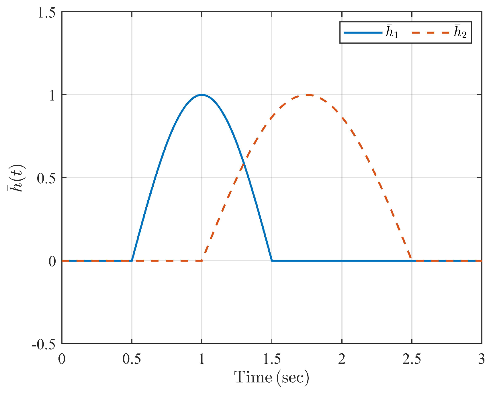
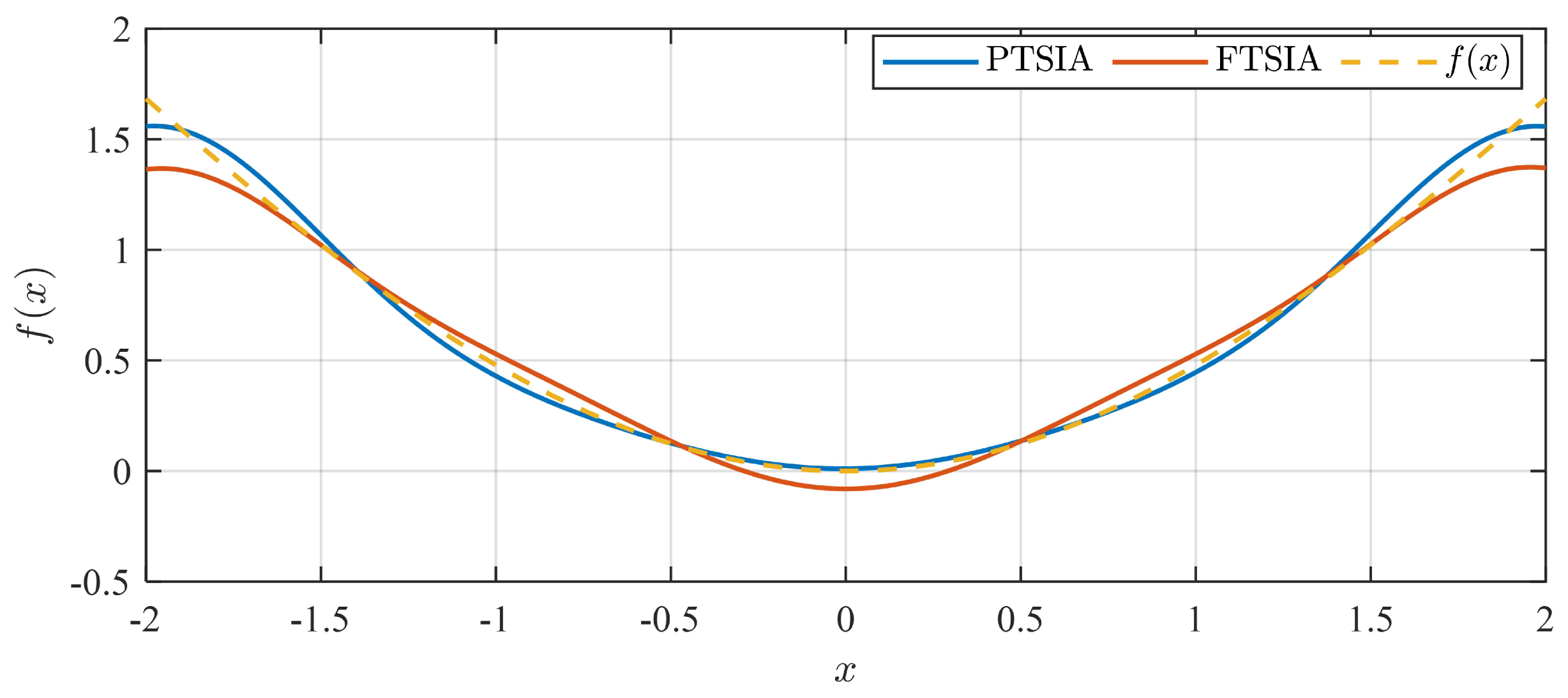
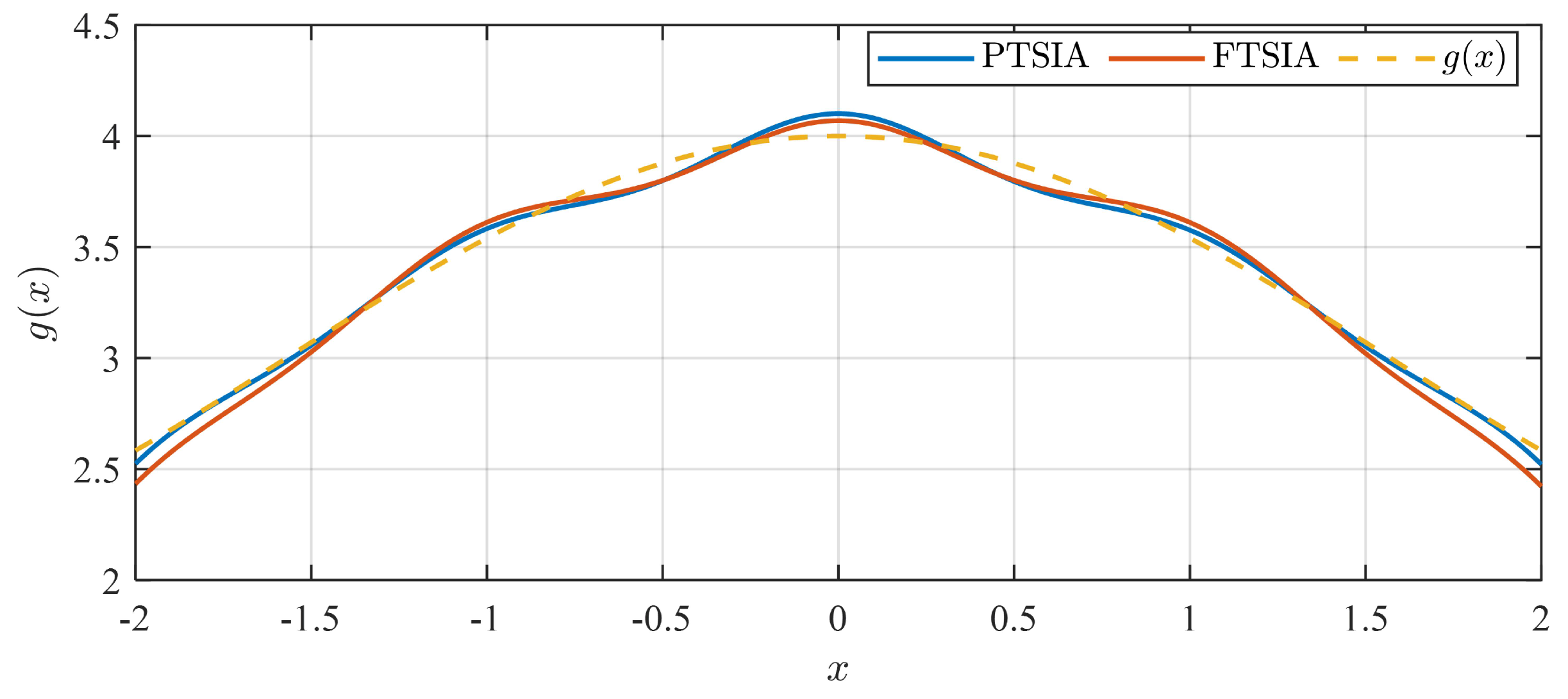
4. Numerical Simulation

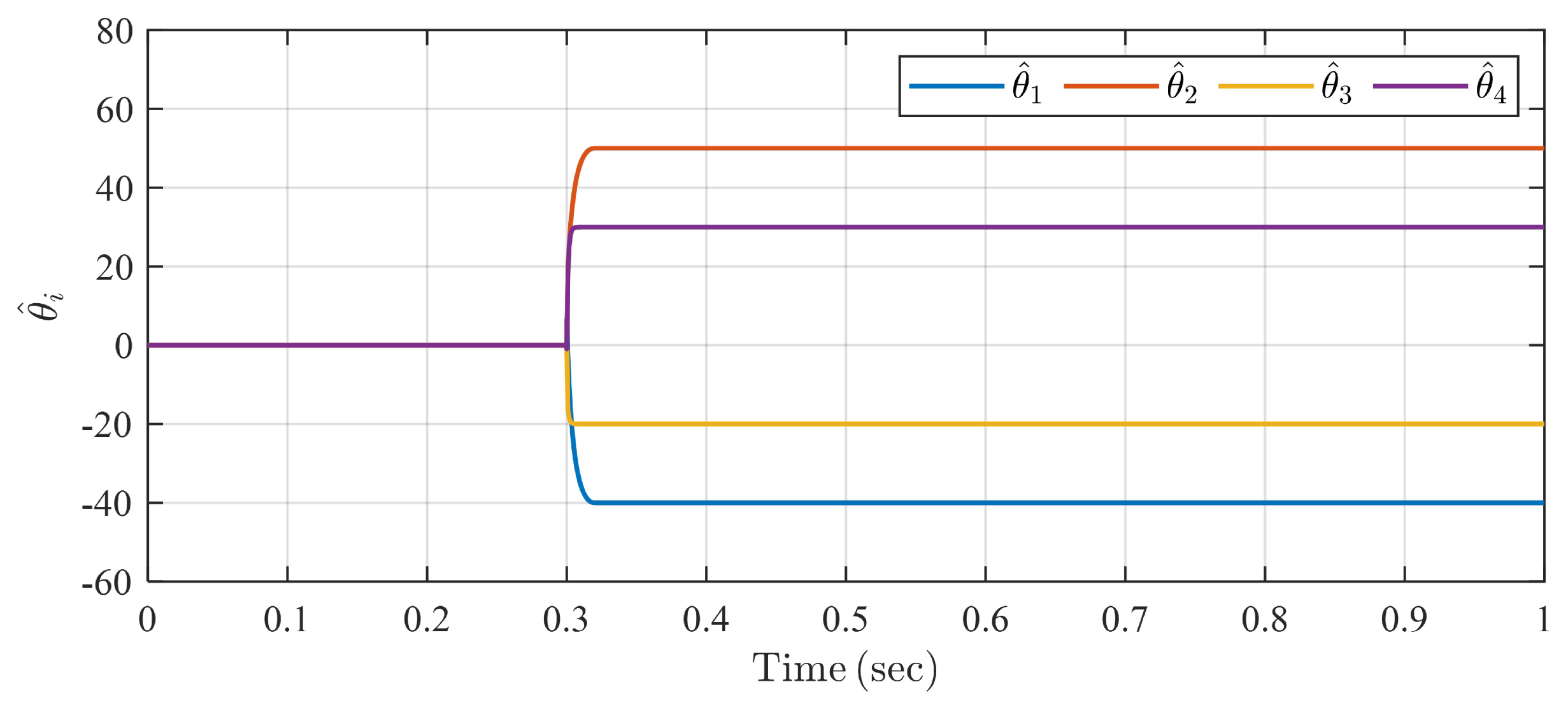
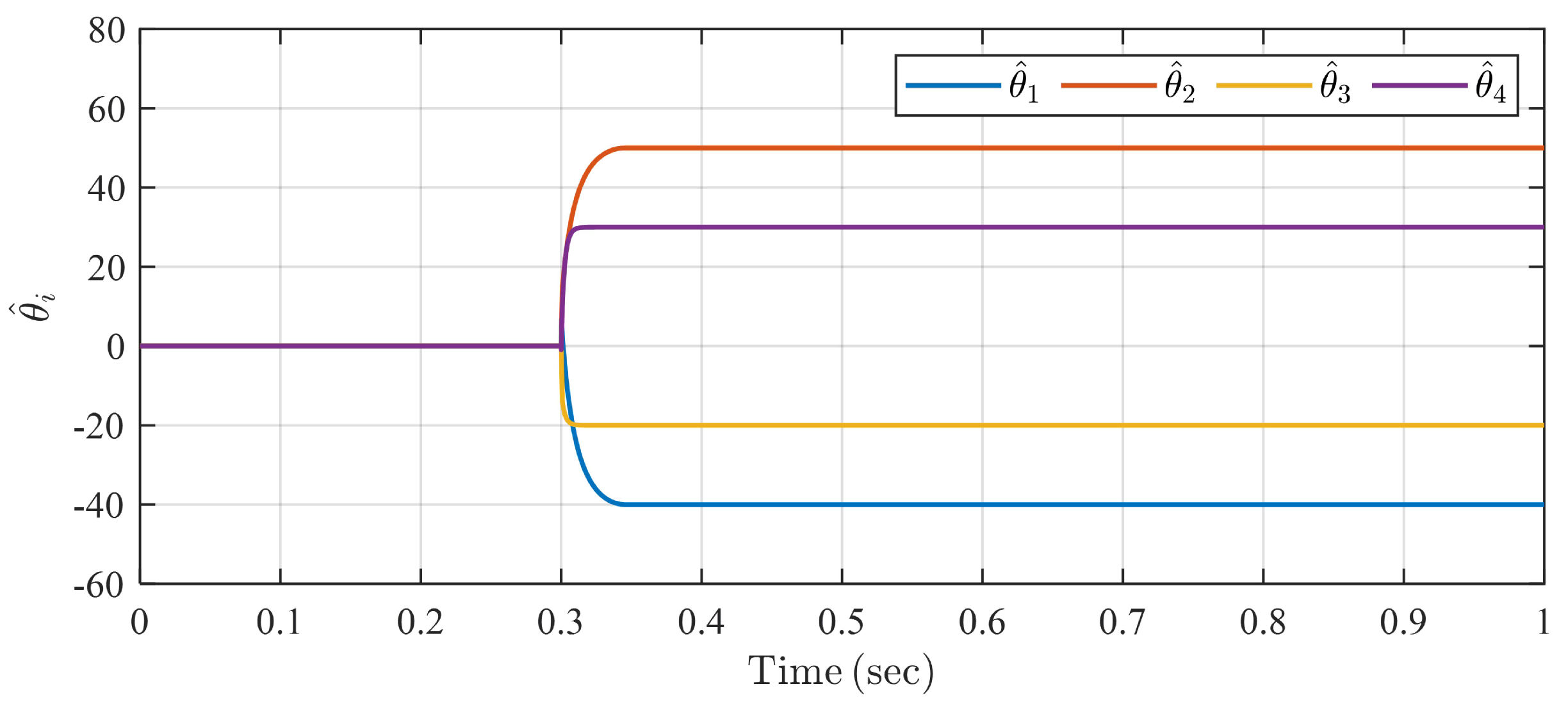
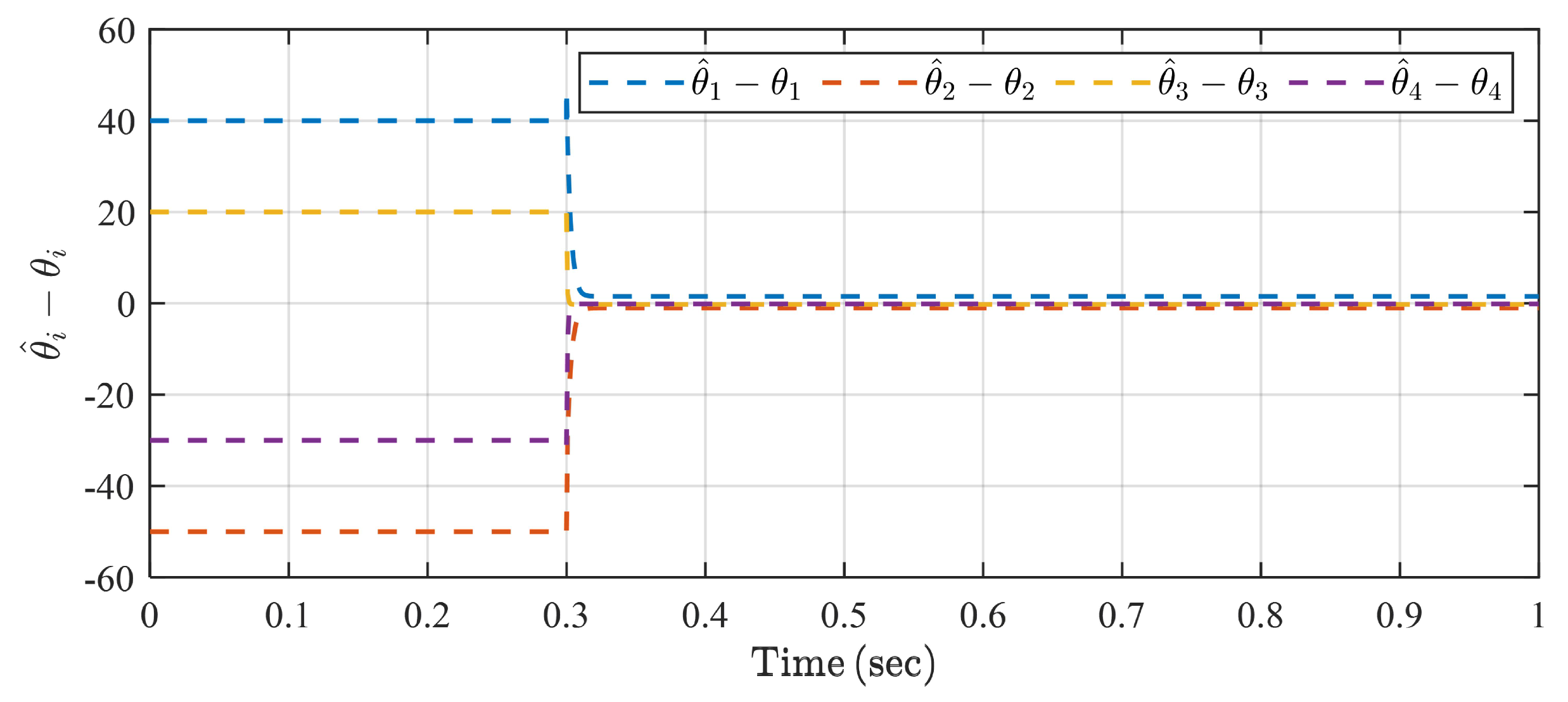
4.1. Simulation of Identification Algorithm without NNAE

Consider the following second-order uncertain system with linearly parametric form:

$$\begin{array}{cc}\hfill {\dot{x}}_1\left(t\right)=& {\theta }_{1}sin\left(x_1\left(t\right)x_2\left(t\right)\right)+{\theta }_2{u}_1\left(t\right)\hfill \\ \hfill {\dot{x}}_2\left(t\right)=& {\theta }_3{x}_2\left(t\right)+{\theta }_4{u}_2\left(t\right)\hfill \end{array}$$

(43)

where ${\theta }_1=-40$, ${\theta }_2=50$, ${\theta }_3=-20$, and ${\theta }_4=30$ are unknown parameters. Then, system (1) can be rewritten in the form of (5) without ${\epsilon }^{\ast }(x\left(t\right),u\left(t\right))$:

$$\begin{array}{c}\hfill \dot{x}\left(t\right)={\Theta }^{\ast T}\xi (x\left(t\right),u\left(t\right))\end{array}$$

(44)

where

$$\begin{array}{c}\hfill x\left(t\right)=\left[\begin{array}{c}{x}_1\left(t\right)\\ x_2\left(t\right)\end{array}\right],{\Theta }^{\ast }=\left[\begin{array}{cc}{\theta }_1& 0\\ 0& {\theta }_3\\ {\theta }_2& 0\\ 0& {\theta }_4\end{array}\right],\xi (x\left(t\right),u\left(t\right))=\left[\begin{array}{c}sin\left(x_1\left(t\right)x_2\left(t\right)\right)\\ x_2\left(t\right)\\ u_1\left(t\right)\\ u_2\left(t\right)\end{array}\right].\end{array}$$

(45)

Update law (23) is applied to generate the precise value of the unknown parameter matrix ${\Theta }^{\ast }$ within the predefined time T. Let the input be $u_1=-0.2x_1\left(t\right)+0.2sin\left(300t\right)+0.8sin\left(x_1\left(t\right)x_2\left(t\right)\right)$, $u_2=0.3x_2\left(t\right)+0.3cos\left(300t\right)$, $x_1\left(0\right)=2$, and $x_2\left(0\right)=-2$. The predefined settling times T are selected as $0.4\mathrm{s}$, $0.7\mathrm{s}$, and $1\mathrm{s}$ for three simulation cases. The other parameters are given by $\mathsf{\Gamma }=10I_4$, $c=100$, and $\eta =0.5$. Historic data $\overline{h}\left(t\right)$, $\overline{l}\left(t\right)$, and $\overline{x}\left(t\right)$ are recorded at every interval ${10}^{-3}\mathrm{s}$ in $t\in [0.1\mathrm{s},0.3\mathrm{s})$. Thus, the numbers of column vectors, p, in the stacks H, L, and X in (17) are all 200, and one can select $\omega$ as $1/4$, $4/7$, and $7/10$, corresponding to the three simulation cases. Denote ${\widehat{\theta }}_i$ as the estimation of ${\theta }_i$ ($i=1,2,3,4$).

The simulation result is presented in Figure 2, Figure 3 and Figure 4. It can be seen that the estimation of unknown parameters, i.e., ${\widehat{\theta }}_i\left(t\right)$ ($i=1,2,3,4$), reaches the corresponding true values ${\theta }_i$ within the desired predefined times T in the three simulation cases. The four estimation errors $|{\widehat{\theta }}_i\left(t\right)-{\theta }_i|$ are all less than ${10}^{-2}$ in the three cases after the predefined settling times T ($i=1,2,3,4$).

In order to test the robustness of the proposed algorithm, system (44) with external disturbances and noises is considered as

$$\begin{array}{c}\hfill \dot{x}\left(t\right)={\Theta }^{\ast T}\xi (x\left(t\right),u\left(t\right))+d_1\left(t\right)\end{array}$$

(46)

with $d_1\left(t\right)={[0.5sin\left(50t\right)+\mathrm{wgn}\left(0.01\right),0.5cos\left(50t\right)+\mathrm{wgn}\left(0.01\right)]}^T$, where $\mathrm{wgn}\left(0.01\right)$ denotes the white Gaussian noise, with power being $0.01\mathrm{dB}\mathrm{W}$. Select the predefined settling time as $T=0.5\mathrm{s}$. The simulation result is shown in Figure 5 and Figure 6. Figure 5 indicates that the estimation of the four unknown parameters can converge to the neighborhood of their true values within T under the proposed identification algorithm. In Figure 6, the steady estimation errors, $|{\widehat{\theta }}_i\left(t\right)-{\theta }_i|$, are 1.5235, 1.0367, 0.2373, and 0.1052, respectively, for $i=1,2,3,4$. The simulation results show the robustness of the proposed system identification algorithm to external disturbances and noise.

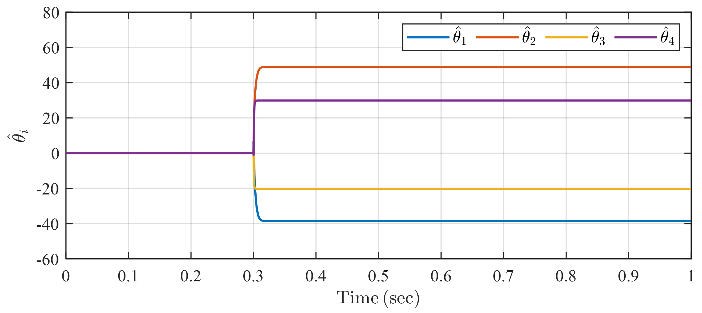
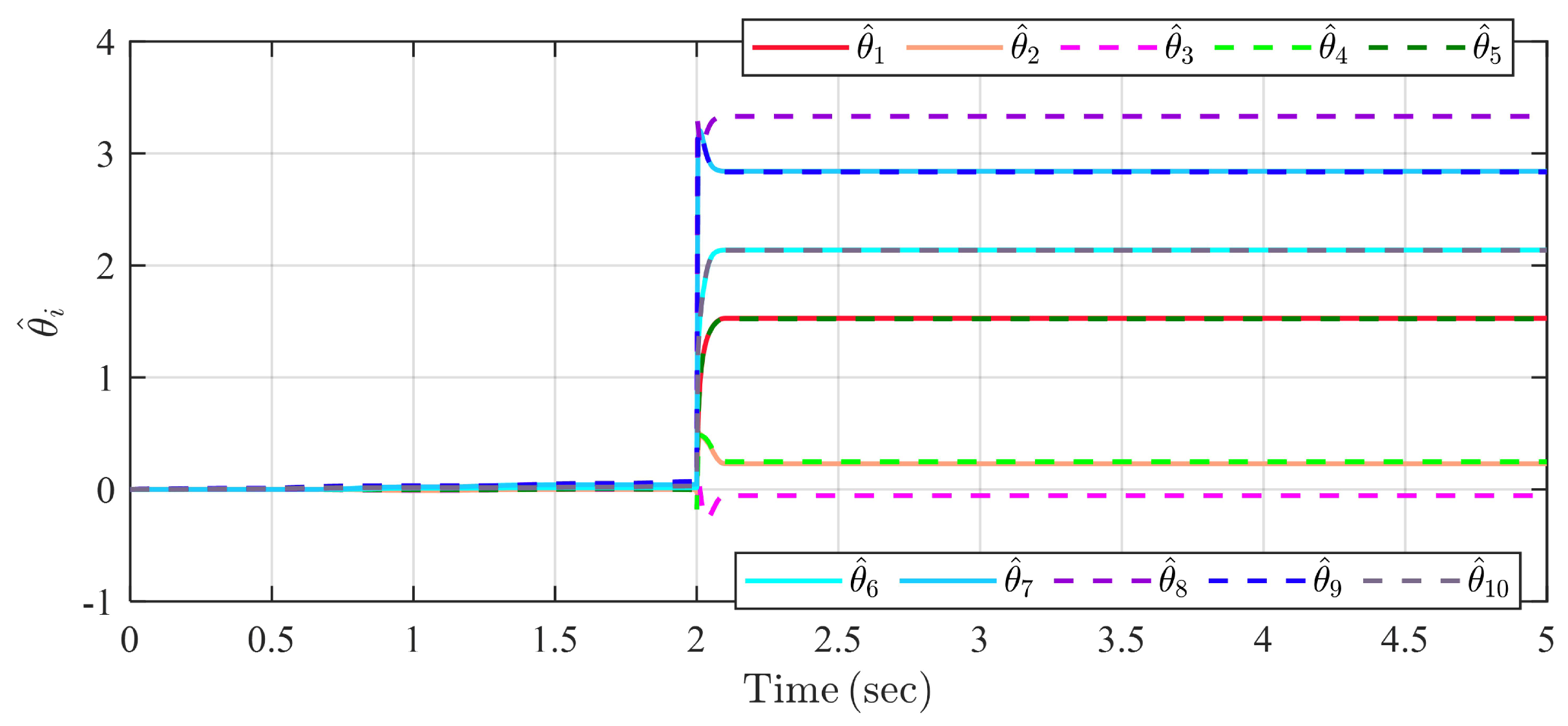
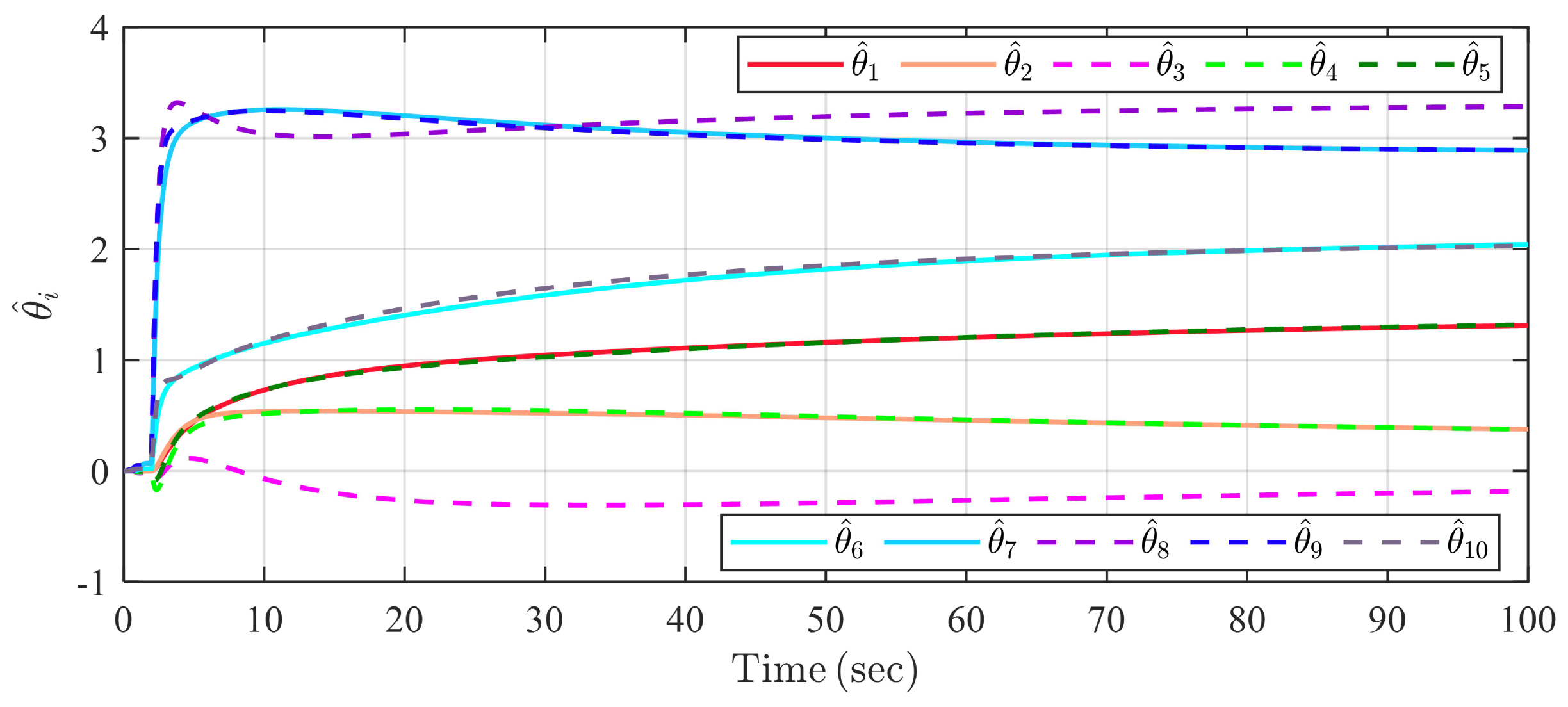
4.2. Simulation of Identification Algorithm with NNAE

Consider the following uncertain system:

$$\begin{array}{c}\hfill \dot{x}\left(t\right)=f\left(x\left(t\right)\right)+g\left(x\left(t\right)\right)u\left(t\right)\end{array}$$

(47)

where $f\left(x\right(t\left)\right)=x\left(t\right)sin\left(0.5x\right(t\left)\right)$ and $g\left(x\right(t\left)\right)=3+cos\left(x\right(t\left)\right)$ are unknown nonlinear functions. Update law (23) with an NN is utilized to approximate the unknown functions $f\left(x\right)$ and $g\left(x\right)$ with small error within the predefined settling time T. Let $x\left(0\right)=1$, and $u=(-100x(t)+200sin(5t)-x(t)sin(0.5x\left(t\right)\left)\right)/(3+cos(x\left(t\right)\left)\right)$. The unknown functions can be approximated by an NN as $f\left(x\right)={\theta }_f^{\ast T}{\xi }_f\left(x\right)+{\epsilon }_f$ and $g\left(x\right)={\theta }_g^{\ast T}{\xi }_g\left(x\right)+{\epsilon }_g$, with ${\theta }_f^{\ast }={[{\theta }_1,\cdots ,{\theta }_5]}^T$ and ${\theta }_g^{\ast }={[{\theta }_6,\cdots ,{\theta }_{10}]}^T$ being unknown weight vectors, where ${\xi }_f={\xi }_g={[{\xi }_1,\cdots ,{\xi }_5]}^T$ is a neural basis function vector, with ${\xi }_j\left(x\right)={\mathrm{e}}^{-|x-{\mu }_j{|}^2/\left(2\sigma \right)}$ ($j=1,...,5$). Select $\sigma =0.5$ and ${[{\mu }_1,\cdots ,{\mu }_5]}^T={[-2,-1,0,1,2]}^T$. The other parameters are given by $\mathsf{\Gamma }=I_{10}$, $c=10$, $\eta =0.5$. The predefined settling time is set as $T=4\mathrm{s}$. Historic data $\overline{h}\left(t\right)$, $\overline{l}\left(t\right)$, and $\overline{x}\left(t\right)$ are recorded at every interval ${10}^{-2}\mathrm{s}$ in $t\in [0.5\mathrm{s},2\mathrm{s})$. Thus, the numbers of column vectors, p, in the stacks H, L, and X in (17) are all 150, and one can select $\omega =0.5$. Denote ${\widehat{\theta }}_i$ as the estimation of ${\theta }_i$ ($i=1,\cdots ,10$). In the simulation, we set ${\widehat{\theta }}_i\left(0\right)=0$$(i=1,\cdots ,10)$. Denote the proposed predefined-time system identification algorithm (23) as PTSIA. Then, the traditional CL-based fixed-time system identification algorithm (FTSIA) in [18] is simulated here for comparison, and it is given by

$$\begin{array}{cc}\hfill \dot{\widehat{\Theta }}=& -{\mathsf{\Gamma }}_1\overline{h}\left(t\right)\left({\lfloor e^T\left(t\right)\rceil }^{{\nu }_1}+{\lfloor e^T\left(t\right)\rceil }^{{\nu }_2}\right)\hfill \\ \hfill & -{\mathsf{\Gamma }}_2\sum _{i=1}^p\overline{h}\left(t_i\right)\left({\lfloor e^T(t,t_i)\rceil }^{{\nu }_1}+{\lfloor e^T(t,t_i)\rceil }^{{\nu }_2}\right)\hfill \end{array}$$

(48)

where ${\mathsf{\Gamma }}_1=1$, ${\mathsf{\Gamma }}_2=1$, ${\nu }_1=0.9$, ${\nu }_2=1.1$, and the other parameters are the same as those in PTSIA.

The simulation results are shown in Figure 7, Figure 8, Figure 9 and Figure 10. The trajectories of the unknown NN weights are stable within the predefined time $T=4\mathrm{s}$ under PTSIA in Figure 7. But it can be seen that they are not stable until about $100\mathrm{s}$ under FTSIA in Figure 8. Thus, it takes more time for FTSIA to approximate the unknown system dynamics compared with PTSIA. Moreover, it is difficult to know and adjust the desired settling time of estimation error with the update law of FTSIA, since the desired settling time boundary does not appear in (48) as an explicit parameter.

Figure 9 and Figure 10 show that the unknown system dynamics $f\left(x\right)$ and $g\left(x\right)$ can be well-approximated by two approaches with acceptable approximation errors. Define two identification errors as $e_f=\parallel E_f\parallel$ and $e_g=\parallel E_g\parallel$, where

$$\begin{array}{cc}\hfill E_f=& {[E_{f(-2)},E_{f(-1.99)},E_{f(-1.98)}\cdots ,E_{f\left(2\right)}]}^T\in {\mathbb{R}}^{400}\hfill \\ \hfill E_g=& {[E_{g(-2)},E_{g(-1.99)},E_{g(-1.98)}\cdots ,E_{g\left(2\right)}]}^T\in {\mathbb{R}}^{400}\hfill \\ \hfill E_{f\left(i\right)}=& (f\left(x\right)-{\widehat{\theta }}_f^T\left(T\right){\xi }_f\left(x\right)){|}_{x=i},i=-2,-1.99,-1.98,\cdots ,2\hfill \\ \hfill E_{g\left(i\right)}=& (g\left(x\right)-{\widehat{\theta }}_g^T\left(T\right){\xi }_g\left(x\right)){|}_{x=i},i=-2,-1.99,-1.98,\cdots ,2.\hfill \end{array}$$

(49)

The parameters $e_f$ and $e_g$ reflect the steady average identification errors for $f\left(x\right)$ and $g\left(x\right)$. Suppose the settling time for FTSIA is $T=100\mathrm{s}$. Then, the simulation result shows that $e_f=0.8186$ and $e_g=0.9368$ for PTSIA, as well as $e_f=1.5495$ and $e_g=1.2787$ for FTSIA. In order to compare the robustness of the two algorithms, system (47) with external disturbances and noise is considered as

$$\begin{array}{c}\hfill \dot{x}\left(t\right)=f\left(x\left(t\right)\right)+g\left(x\left(t\right)\right)u\left(t\right)+d_2\left(t\right).\end{array}$$

(50)

If $d_2\left(t\right)$ is selected as $0.1sin\left(20t\right)+\mathrm{wgn}\left(0.01\right)$, we obtain that $e_f=1.0063$ and $e_g=1.2105$ for PTSIA, as well as $e_f=1.4816$ and $e_g=1.2523$ for FTSIA. If $d_2\left(t\right)$ is selected as $0.2sin\left(10t\right)+\mathrm{wgn}\left(0.02\right)$, we obtain that $e_f=1.0326$ and $e_g=1.7435$ for PTSIA, as well as $e_f=3.2225$ and $e_g=1.7614$ for FTSIA. Therefore, one can conclude that the proposed PTSIA is superior to the traditional FTSIA in terms of approximation speed, identification accuracy, and settling time adjustment.

Further, a sensitivity test is provided to analyze the performance of the proposed algorithm to parameter variations. The robustness and the identification accuracy can be reflected by the steady average identification errors $e_f$ and $e_g$. Then, an identification efficiency parameter $T_s$ is defined as the time after which the inequalities $|{\widehat{\theta }}_i\left(t\right)-{\widehat{\theta }}_i\left(T\right)|\le {10}^{-4}$ always hold ($i=1,\cdots ,10$), indicating the time when the identification algorithm enters the steady state. The identification efficiency is higher if $T_s$ is shown to be smaller.

The simulation results of the performance of system (47) under variations in parameters $\eta$, c, $\omega$, and $\mathsf{\Gamma }$ are summarized in

Table 2. Performance of system (47) under $T=10\mathrm{s}$, $\omega =0.8$, $c=10$, $\mathsf{\Gamma }=I_{10}$, and different $\eta$.

Parameters	$\mathit{\eta }=0.1$	$\mathit{\eta }=0.3$	$\mathit{\eta }=0.5$	$\mathit{\eta }=0.7$	$\mathit{\eta }=0.9$
$e_f$	0.8182	0.8182	0.8182	0.8186	0.8183
$e_g$	0.9357	0.9357	0.9358	0.9366	0.9360
$T_s\left(\mathrm{s}\right)$	2.59	2.39	2.16	2.08	2.03

,

Table 3. Performance of system (47) under $T=10\mathrm{s}$, $\eta =0.4$, $\omega =0.8$, $\mathsf{\Gamma }=I_{10}$, and different c.

Parameters	$\mathit{c}=1$	$\mathit{c}=5$	$\mathit{c}=10$	$\mathit{c}=50$	$\mathit{c}=300$
$e_f$	18.9727	1.7258	0.8182	0.7804	0.7616
$e_g$	5.5829	1.2126	0.9358	0.9314	0.9312
$T_s\left(\mathrm{s}\right)$	8.49	2.19	2.25	2.43	2.47

,

Table 4. Performance of system (47) under $T=10\mathrm{s}$, $\eta =0.5$, $c=20$, $\mathsf{\Gamma }=I_{10}$, and different $\omega$.

Parameters	$\mathit{\omega }=0.1$	$\mathit{\omega }=0.2$	$\mathit{\omega }=0.4$	$\mathit{\omega }=0.6$	$\mathit{\eta }=0.8$
$e_f$	0.8157	0.8157	0.8157	0.8157	0.8157
$e_g$	0.9304	0.9302	0.9302	0.9302	0.9302
$T_s\left(\mathrm{s}\right)$	9.03	8.06	6.12	4.17	2.22

and

Table 5. Performance of system (47) under $T=10\mathrm{s}$, $\eta =0.6$, $c=8$, $\omega =0.5$, and different $\mathsf{\Gamma }$.

Parameters	$\mathbf{\Gamma }=0.01{\mathit{I}}_{10}$	$\mathbf{\Gamma }=0.1{\mathit{I}}_{10}$	$\mathbf{\Gamma }={\mathit{I}}_{10}$	$\mathbf{\Gamma }=10{\mathit{I}}_{10}$	$\mathbf{\Gamma }=100{\mathit{I}}_{10}$
$e_f$	0.8233	0.8233	0.8226	0.8233	0.8233
$e_g$	0.9550	0.9550	0.9538	0.9550	0.9550
$T_s\left(\mathrm{s}\right)$	5.10	5.10	5.10	5.10	5.10

, respectively. It can be seen from Table 2 and Table 5 that the variations in $\eta$ and $\mathsf{\Gamma }$ have little impact on the identification accuracy and efficiency. Table 3 shows that the identification accuracy is improved with increases in the parameter c. But the improvement is limited if $c>10$. The identification error increases significantly if $c<5$. Table 4 shows that the real settling time of the algorithm is shortened with increases in the parameter $\omega$. But the real settling times under different $\omega$ are all less than the predefined one, $T=10\mathrm{s}$.

5. Conclusions and Future Work

This paper proposes a CL-based two-stage predefined-time system identification algorithm. The algorithm takes effect under a finite-rank condition rather than the infinite PE condition. It is proven that the estimation error converges to zero for linearly parameterized uncertain systems, or it converges into the neighborhood of zero for unknown systems modeled by an NN, within a predefined settling time. The desired settling time boundary is uniform to initial estimation errors, known a priori by users compared with traditional related studies. Simulations verify the effectiveness and superiority of the proposed algorithm. In future work, CL-based predefined-time identification for distributed uncertain systems will be studied.

References

1. Wang, J.; Efimov, D.; Bobtsov, A.A. On robust parameter estimation in finite-time without persistence of excitation. IEEE Trans. Autom. Control 2020, 65, 1731–1738. [Google Scholar] [CrossRef]
2. Krstic, M.; Kokotovic, P.V.; Kanellakopoulos, I. Nonlinear and Adaptive Control Design, 1st ed.; Wiley-Interscience: New York, NY, USA, 1995. [Google Scholar]
3. Djaneye-Boundjou, O.; Ordonez, R. Gradient-based discrete-time concurrent learning for standalone function approximation. IEEE Trans. Autom. Control 2020, 65, 749–756. [Google Scholar] [CrossRef]
4. Chowdhary, G.V.; Johnson, E.N. Theory and flight-test validation of a concurrent-learning adaptive controller. J. Guid. Control. Dyn. 2011, 34, 592–607. [Google Scholar] [CrossRef]
5. Chowdhary, G.; Yucelen, T.; Mühlegg, M.; Johnson, E.N. Concurrent learning adaptive control of linear systems with exponentially convergent bounds. Int. J. Adapt. Control Signal Process. 2013, 27, 280–301. [Google Scholar] [CrossRef]
6. Kamalapurkar, R.; Reish, B.; Chowdhary, G.; Dixon, W.E. Concurrent learning for parameter estimation using dynamic state-derivative estimators. IEEE Trans. Autom. Control 2017, 62, 3594–3601. [Google Scholar] [CrossRef]
7. Parikh, A.; Kamalapurkar, R.; Dixon, W.E. Integral concurrent learning: Adaptive control with parameter convergence using finite excitation. Int. J. Adapt. Control Signal Process. 2019, 33, 1775–1787. [Google Scholar] [CrossRef]
8. Bell, Z.I.; Nezvadovitz, J.; Parikh, A.; Schwartz, E.M.; Dixon, W.E. Global exponential tracking control for an autonomous surface vessel: An integral concurrent learning approach. IEEE J. Ocean. Eng. 2020, 45, 362–370. [Google Scholar] [CrossRef]
9. Du, Y.; Liu, F.; Qiu, J.; Buss, M. Online identification of piecewise affine systems using integral concurrent learning. IEEE Trans. Circuits Syst. I Regul. Pap. 2021, 68, 4324–4336. [Google Scholar] [CrossRef]
10. Zhao, L.; Zhi, J.; Yin, N.; Chen, Y.; Li, J.; Liu, J. Performance improvement of finite time parameter estimation with relaxed persistence of excitation condition. J. Electr. Eng. Technol. 2019, 14, 931–939. [Google Scholar] [CrossRef]
11. Na, J.; Mahyuddin, M.N.; Herrmann, G.; Ren, X.; Barber, P. Robust adaptive finite-time parameter estimation and control for robotic systems. Int. J. Robust Nonlinear Control 2015, 25, 3045–3071. [Google Scholar] [CrossRef]
12. Wang, S.; Na, J.; Yu, H.; Chen, Q. Finite time parameter estimation-based adaptive predefined performance control for servo mechanisms. ISA Trans. 2019, 87, 174–186. [Google Scholar] [CrossRef] [PubMed]
13. Yang, C.; Jiang, Y.; He, W.; Na, J.; Li, Z.; Xu, B. Adaptive parameter estimation and control design for robot manipulators with finite-time convergence. IEEE Trans. Ind. Electron. 2018, 65, 8112–8123. [Google Scholar] [CrossRef]
14. Yang, C.; Jiang, Y.; Na, J.; Li, Z.; Cheng, L.; Su, C.Y. Finite-time convergence adaptive fuzzy control for dual-arm robot with unknown kinematics and dynamics. IEEE Trans. Fuzzy Syst. 2019, 27, 574–588. [Google Scholar] [CrossRef]
15. Vahidi-Moghaddam, A.; Mazouchi, M.; Modares, H. Memory-augmented system identification with finite-time convergence. IEEE Control Syst. Lett. 2021, 5, 571–576. [Google Scholar] [CrossRef]
16. Tatari, F.; Modares, H.; Panayiotou, C.; Polycarpou, M. Finite-time distributed identification for nonlinear interconnected systems. IEEE/CAA J. Autom. Sin. 2022, 9, 1188–1199. [Google Scholar] [CrossRef]
17. Wu, Z.; Guo, J.; Liu, B.; Ni, J.; Bu, X. Composite learning adaptive dynamic surface control for uncertain nonlinear strict-feedback systems with fixed-time parameter estimation under sufficient excitation. Int. J. Robust Nonlinear Control 2021, 31, 5865–5889. [Google Scholar] [CrossRef]
18. Tatari, F.; Mazouchi, M.; Modares, H. Fixed-time system identification using concurrent learning. IEEE Trans. Neural Netw. Learn. Syst. 2023, 34, 4892–4902. [Google Scholar] [CrossRef] [PubMed]
19. Bobtsov, A.; Nikolaev, N.; Ortega, R.; Efimov, D. State observation of ltv systems with delayed measurements: A parameter estimation-based approach with fixed convergence time. Automatica 2021, 131, 109674. [Google Scholar] [CrossRef]
20. Gallegos, J.A.; Aguila-Camacho, N. Necessary and sufficient conditions for convergence of drem-based estimators with applications in adaptive control. Automatica 2022, 146, 110597. [Google Scholar] [CrossRef]
21. Jiménez-Rodríguez, E.; Muñoz-Vázquez, A.J.; Sánchez-Torres, J.D.; Defoort, M.; Loukianov, A.G. A lyapunov-like characterization of predefined-time stability. IEEE Trans. Autom. Control 2020, 65, 4922–4927. [Google Scholar] [CrossRef]
22. Ferrara, A.; Incremona, G.P. Predefined-time output stabilization with second order sliding mode generation. IEEE Trans. Autom. Control 2021, 66, 1445–1451. [Google Scholar] [CrossRef]
23. Gómez-Gutiérrez, D.; Aldana-López, R.; Seeber, R.; Angulo, M.T.; Fridman, L. An arbitrary-order exact differentiator with predefined convergence time bound for signals with exponential growth bound. Automatica 2023, 153, 110995. [Google Scholar] [CrossRef]
24. Seeber, R.; Haimovich, H.; Horn, M.; Fridman, L.M.; De Battista, H. Robust exact differentiators with predefined convergence time. Automatica 2021, 134, 109858. [Google Scholar] [CrossRef]
25. Yang, X.; Fan, X.; Long, F.; Li, G. Predefined-time robust control with formation constraints and saturated controls. Nonlinear Dyn. 2022, 110, 2535–2554. [Google Scholar] [CrossRef]
26. Wang, W.; Hou, M.; Liu, B. Fault-tolerant adaptive asymptotic attitude tracking control for a rigid spacecraft. Iran. J. Sci.-Technol.-Trans. Electr. Eng. 2021, 45, 1383–1394. [Google Scholar] [CrossRef]
27. Na, J.; Huang, Y.; Liu, T.; Zhu, Q. Reinforced adaptive parameter estimation with prescribed transient convergence performance. Syst. Control Lett. 2021, 149, 104880. [Google Scholar] [CrossRef]
28. Dastres, H.; Ebrahimi, S.M.; Malekzadeh, M.; Gordillo, F. Robust adaptive parameter estimator design for a multi-sinusoidal signal with fixed-time stability and guaranteed prescribed performance boundary of estimation error. J. Frankl. Inst. 2023, 360, 223–250. [Google Scholar] [CrossRef]
29. Wu, Z.; Ma, M.; Xu, X.; Liu, B.; Yu, Z. Predefined-time parameter estimation via modified dynamic regressor extension and mixing. J. Frankl. Inst. 2021, 358, 6897–6921. [Google Scholar] [CrossRef]
30. Yang, X. Some trace inequalities for operators. J. Aust. Math. Soc. 1995, 58, 281–286. [Google Scholar] [CrossRef]
31. Ma, R.; Fu, L.; Fu, J. Prescribed-time tracking control for nonlinear systems with guaranteed performance. Automatica 2022, 146, 110573. [Google Scholar] [CrossRef]
Figure 1. Trajectories of signals h ¯ 1 ( t ) and h ¯ 2 ( t ) in (20).
Electronics 13 01460 g001
Figure 2. Trajectories of estimation of unknown parameters for system (43) under T = 0.4 s .
Electronics 13 01460 g002
Figure 3. Trajectories of estimation of unknown parameters for system (43) under T = 0.7 s .
Electronics 13 01460 g003
Figure 4. Trajectories of estimation of unknown parameters for system (43) under T = 1 s .
Electronics 13 01460 g004
Figure 5. Trajectories of estimation of unknown parameters for system (43) with disturbances and noises under T = 0.5 s .
Electronics 13 01460 g005
Figure 6. Trajectories of parameter estimation errors for system (43) with disturbances and noises under T = 0.5 s .
Electronics 13 01460 g006
Figure 7. Trajectories of estimation of unknown NN weights under PTSIA for system (47).
Electronics 13 01460 g007
Figure 8. Trajectories of estimation of unknown NN weights under FTSIA for system (47).
Electronics 13 01460 g008
Figure 9. Trajectories of unknown drift dynamics and their approximation for system (47).
Electronics 13 01460 g009
Figure 10. Trajectories of unknown input dynamics and their approximation for system (47).
Electronics 13 01460 g010