

Boundary Protection Based on S-Transform Considering Fault Factors

School of Mechanical and Electrical Engineering, Guilin University of Electronic Technology, Guilin 541004, China
*
Author to whom correspondence should be addressed.
Electronics 2024, 13(8), 1464; https://doi.org/10.3390/electronics13081464
Submission received: 29 February 2024
/
Revised: 8 April 2024
/
Accepted: 9 April 2024
/
Published: 12 April 2024
(This article belongs to the Special Issue Advanced Fault Detection, Diagnosis and Control in Industrial Electronics)
Abstract
:Boundary protection is a protection that takes advantage of the characteristic that signals will be attenuated when passing through the “line boundary”. The location of the traps and current transformers in the structure of extra-high voltage (EHV) transmission lines makes it difficult to apply current-based travelling wave protection in engineering practice. If the protection is put into use, it is necessary to carry out a large number of engineering modifications to the existing transmission lines, which greatly increases the economic cost. And after simulation, the protection will be misjudged under weak fault conditions, and it has low reliability. After analyzing the influence of fault factors, a boundary protection method using high-frequency voltage component energy is proposed. The fault signal is processed by S-transform, and the transient voltage energy is normalized with the initial fault phase and transition resistance. The reduced characteristic quantity is used to construct a criterion to judge the fault condition of the protection line. This protection eliminates the influence of fault factors on transient protection. The ATP-Draw 6.0 simulation results based on the proposed protection scheme show that the protection scheme can distinguish internal and external faults, and can work normally under weak faults with high reliability.
1. Introduction
In China, long-distance transmission has become a general trend, and relay protection devices are required to have higher values in the “four characteristics” [1,2,3,4,5]. Although relay protection based on power frequency is still the first choice in engineering, the quick action can not meet the operation requirements of extra-high voltage (EHV) transmission lines. A wealth of fault information is generated when the line fails. The relay protection scheme composed of transient components can quickly remove faults, which is suitable for EHV transmission lines [6].
Traveling wave protection also belongs to transient protection, which uses the information contained in voltage and current during line fault to form protection criteria. In order to be more convenient in the analysis of the travelling wave process, the conclusions drawn are based on the uniform lossless conductor, and the travelling wave protection established therefrom is not applicable to non-uniform transmission lines. In the reference [7], the sampling rate is taken into account, which solves the problem that the proposed double-ended travelling wave protection cannot accurately discriminate between in-zone and out-of-zone faults after it has been applied to the non-uniform lines. In fact, the power system is complex, and there are relations between transient components. Information entropy can be used to characterize the overall distribution characteristics of signals, and fault information contained in transient components can be extracted by information measure. Reference [8] theoretically discusses the difference between the energy of fault current and voltage components inside and outside the line area, thus constructing entropy as the criterion of longitudinal direction protection. However, this kind of signal processing method based on mathematical transformation has a large amount of calculation and is difficult to be widely used. Reference [9] analyzes the frequency distribution principle of traveling waves at different fault locations, the energy difference in different frequency bands is amplified when wavelet packet energy is integrated into frequency as transient energy. In addition to the construction scheme of protection criterion by using the polarity, amplitude and energy of traveling wave, we can also start with the phase of traveling wave. Reference [10] introduces the concept of traveling wave phase difference, and constructs the protection criterion by comparing the magnitude relationship between phase difference and setting value. According to the simulation results, the protection is quick, but there is an error when the line distance is short. Bus fault will cause damage to related electrical equipment, and may cause regional power failure [11]. Reference [12] introduces the ratio of comprehensive active driving quantity to active braking quantity to specify the protection criterion. Single-ended traveling wave protection does not need communication channel and time synchronization. Compared with double-ended traveling wave protection, it has lower investment cost, higher economic benefit and higher research value [13].
With the rapid development of computer technology [14], the research of transient protection is pushed to a new climax with the addition of mathematical processing tools. The amplitude, polarity, phase, and frequency of fault signals are fully utilized. The constructed protection scheme has high-speed action performance and the judgment results for different faults are more accurate. However, these research schemes focus on the utilization of fault information and the precision control of protection criteria, and fail to solve the influence of fault factors on transient protection schemes in principle, which leads to low reliability of transient protection. Additionally, the effects of the fault factors are not considered carefully enough. When verifying the influence of the initial fault angle on the protection scheme, almost all of them start from 30°, and rarely consider the case where the initial fault angle crosses the vicinity of the zero point [15]. When verifying the effect of transition resistance on the protection scheme, the highest value selected is about 150 , and high impedance is less considered [16,17]. For single-phase ground faults, the transition resistance can be up to 300 at 500 kV.
At present, travelling wave protection mainly uses current travelling wave information to construct protection criteria. However, there are traps in China’s ultra-high voltage transmission line system structure. The current transformer is installed between the bus and the trap, so whether the fault occurs in the area or out of the area, the fault component will pass through the trap. The frequency components of the signal located within the trap’s resistance band are attenuated after passing through the trap, which has a certain impact on the identification of faults in and out of the zone. Therefore, if the travelling wave protection constructed by current travelling wave is put into use, it is necessary to modify the existing line, i.e., to swap the position of the detector and current transformer, which will increase the huge economic cost.
In this paper, an S-transform-based boundary protection considering fault factors is proposed. The voltage information is transformed by S-transform, and the data of specific frequency are extracted to obtain the single-frequency voltage energy, and then the voltage energy is reduced to eliminate the influence of the fault factors, and the criterion is established according to the reduced value of voltage energy when an internal or external fault occurs. The results obtained after selecting a large number of fault initial angles and transition resistors for simulation at different fault locations show that the scheme has good feasibility, high reliability, and quick action.
2. Frequency Characteristics of Extra-High Voltage (EHV) Transmission Lines
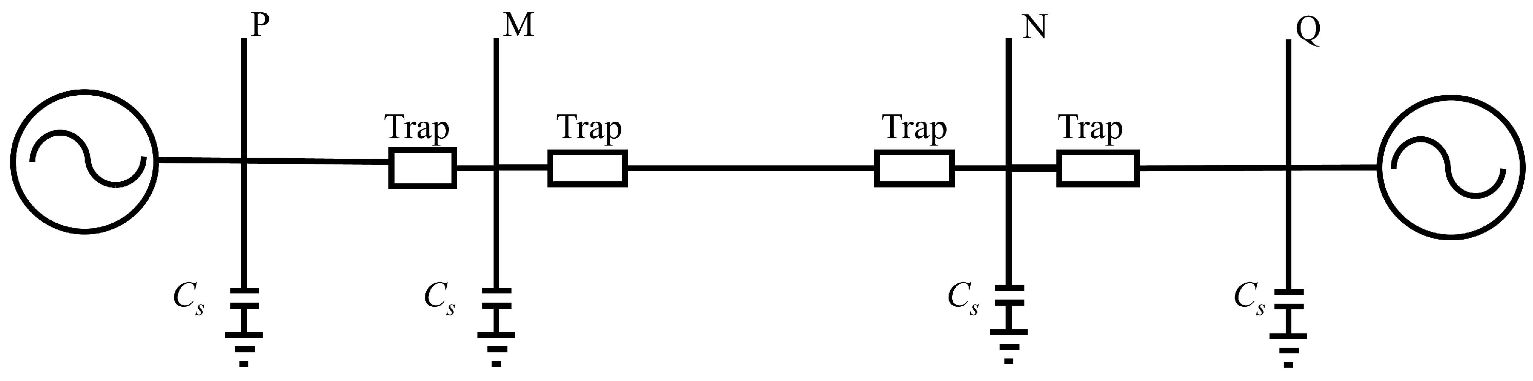
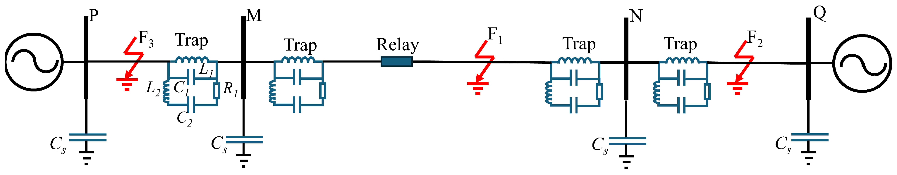
Bus-to-ground capacitance has an important influence on the distribution of transient components, which cannot be ignored in EHV transmission lines. Generally, the capacitance to ground installed on EHV alternating current (AC) transmission lines ranges from 2000 pF to 0.1 μF. The greater the capacitance between bus and ground, the greater the transmission attenuation of signal, and the transmission and reflection ability of signals enhances with the increase in frequency. The trap and the bus capacitance to ground together constitute the “line boundary”. The trap consists of a main coil and a tuning device, and the model is shown in Figure 1 [18]. The trap is connected in series between the bus and the transmission line protection installation, which is an important equipment for high frequency protection and communication signal transmission. Inductor is the main coil for carrying power frequency current. Inductor , capacitor , capacitor , and resistance together form a tuning device, which forms a resonant circuit with the main coil, and presents high impedance to high-frequency signals in a certain frequency band, thus preventing high-frequency signals from being transmitted in unnecessary directions. In this paper, the parameters of the trap designed in reference [18] are used to design the transmission system. According to this document, the blocking frequency band of the wave blocker is [62.3 kHz, 384.7 kHz], and the transient signal in this frequency band is seriously attenuated. In order to make the high-frequency signals generated inside and outside the area not affect each other, traps should be installed at both ends of the adjacent buses where the protected lines are installed, as shown in Figure 2 [19].
3. Transmission Line Protection Based on Fault Factors
3.1. Fundamental Principle
When the transient component passes through the line boundary, the frequency signals above 10 kHz within the signal are called high frequency [20]. As known from the previous section, the detector will exhibit a high-resistance characteristic for high-frequency components within the stopband [62.3 kHz, 384.7 kHz]. When an in-area fault occurs, all high-frequency components can be detected. Otherwise, the components received by the protection device will be much less. Therefore, by comparing the high-frequency energy extracted and the set threshold value when the line fails, the protection scheme is formed. In this paper, the voltage mode energy is selected as the fault component.
The above basic principle is feasible in theory, but there are some defects. When the initial fault angle is about 0, the forward-traveling wave energy of the voltage will be greatly reduced, and with the increase in transition resistance, the forward-traveling wave energy of the voltage will decrease. In this case, there may be an overlap in the range of voltage forward-traveling wave energy values between the inner and outer regions. The data in Table 1 show the energy calculated by integrating the voltage travelling wave amplitude at the M-terminal of the line using the initial travelling wave arriving at the protection mounting for a period of 0.5 ms (the voltage energy is calculated according to Equation (15)). As shown in Table 1, the range of voltage forward-traveling wave energy values is – in the inner region and – in the outer region. There is numerical overlapping of the voltage travelling wave energy during faults inside and outside the zone. When the initial angle of the fault is 0° the energy range of the fault outside the zone is –, in other cases the energy range of the fault outside the zone is –, which completely overlaps with the range of the voltage travelling wave energy during faults inside the zone. This will affect the value of the threshold; in turn, protection cannot act correctly. And from Table 1, it can be seen that 85% of the values of the voltage energy of the out-of-area faults are within the energy range of the in-area faults, which means that the probability of misjudgement can be as high as 85%, which seriously affects the protection reliability. Therefore, voltage energy can be reduced according to the fault factors, and all fault conditions can be reduced to the same situation, which is beneficial to the setting of protection criteria.
3.2. Initial Angle
Let the resistance per unit length of the line be x and the capacitance per unit length be b, so the phase coefficient . Therefore, the initial fault angle of the fault point can be calculated by monitoring the phase when the protection installation site fails and calculating the distance of the fault point. The specific calculation steps are as follows: ① Calculate the fault distance L from the beginning of the fault to the protection device site; ② Detect the fault angle of the installation place; ③ Calculate the phase coefficient L of the line; ④ Calculate the fault initial angle , At present, many accurate methods have been developed for fault location [21,22]. In the ranging scheme provided in reference [23], the error is small at different fault factors. The loop equations are derived in the frequency domain using the amount of change in phase voltage and phase current before and after the fault to derive the formula for the phase voltage at the protected installation point after the fault and the fault distance. Then the equation is switched to the time domain for time integration to find the fault distance between the fault point and the protection installation. The phase angle of the fault current at both ends of the fault point is one of the factors affecting the accuracy of the distance measurement scheme, and the distance measurement scheme makes use of the change in the voltage at the single end of the protection to compensate for the error caused by the inconsistency in the phase angle of the fault current components at both ends of the fault point, which improves the accuracy of the measurement. The deviation is within 3% in the low-resistance fault state, within 5% in the high-resistance fault state, and the error distance is less than 3 km. Therefore, using this fault location algorithm to calculate the initial fault angle, the calculation accuracy is less than .
3.3. Transition Resistance
In order to simplify the analysis, the transition resistance is calculated by using the two-terminal -type single-phase transmission parameter system model [24], as shown in Figure 3.
Let the line be uniform, and the resistance, capacitance, and inductance per unit length are r, c, and l, respectively. The total length of the line is L. After simplifying KCL equation and KVL equation of fault point F, we can obtain
Among them, , , and are voltage and current time domain signals measured from bus M and bus N, respectively. is the voltage time domain signal measured at the fault point, and is the current time domain signal flowing through the transition resistor . If , , , and are substituted into Formula (1), and can be obtained, and the transition resistance is
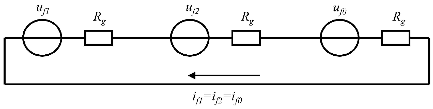
Three-phase power system can be decomposed into three independent mode networks: mode 0, mode 1 and mode 2. Then solve the transition resistance by similar processing methods as single-phase systems. Each mode network can be equivalent to the structure shown in Figure 3. For different modular networks, an expression similar to Formula (1) can be written as Formula (3).
where k = 0, 1, 2. Different fault conditions determine different compound mode networks, and then determine different expressions for solving transition resistance. Taking a single-phase grounding fault as an example, the composite mode network obtained according to the fault boundary conditions is shown in Figure 4. The expression of transition resistance obtained from Figure 4 is
By analyzing the compound mode network of other fault conditions, the following conclusions are drawn. When two phases pass through the grounding short circuit fault of the transition resistance, the expression of the transition resistance is
When two phases pass through the short circuit fault of the transition resistance, the expression of the transition resistance is
Three-phase short circuit is a symmetrical fault, which can be directly analyzed by the circuit in Figure 3. The expression of transition resistance is
3.4. S-Transform
The S-transform of the signal is defined as follows [25]:
where is a Gaussian window, . As the frequency increases, the width of Gaussian window becomes narrower, so S-transform has good time-frequency resolution characteristics. i is an imaginary unit. If
Then the discrete S-transform of the signal can be expressed as:
Then, the collected discrete signal is subjected to S-transform by Formulas (11) and (12), and the transformation result is recorded as an S-matrix, with columns corresponding to sampling time points and rows corresponding to frequencies. The frequency corresponding to the nth line is:
where is the sampling frequency. Let the number of sampling points be n, and select the ith single-frequency traveling wave information for energy calculation. The result can be expressed as follows:
In this paper, the sampling frequency is 200 kHz. A basic rule of thumb is that there is a big gap between the fault energy of 100 kHz, which is suitable for constructing protection criteria. The signal is processed by the S-transform, the 100 kHz voltage information is extracted. The traveling wave energy within 0.5 ms (N = 100) is obtained by Formula (14).
3.5. On the Reduction of Fault Factors
According to the basic principle, the trap can attenuate the high frequency components. Therefore, taking Figure 3 as an example, the -mode component of the voltage at the M-end of the line is extracted as , and the high-frequency component at 100 kHz is extracted, and the S-transform energy is calculated. The result is expressed as follows: for energy calculation. The result can be expressed as follows:
Then the is reduced according to the initial fault angle and transition resistance, and is obtained. results are expressed as:
where is the reduction coefficient about fault factors. Summarized by simulation data, the expression is deduced as follows:
where is the initial fault angle and is the transition resistance.
4. Simulation Example
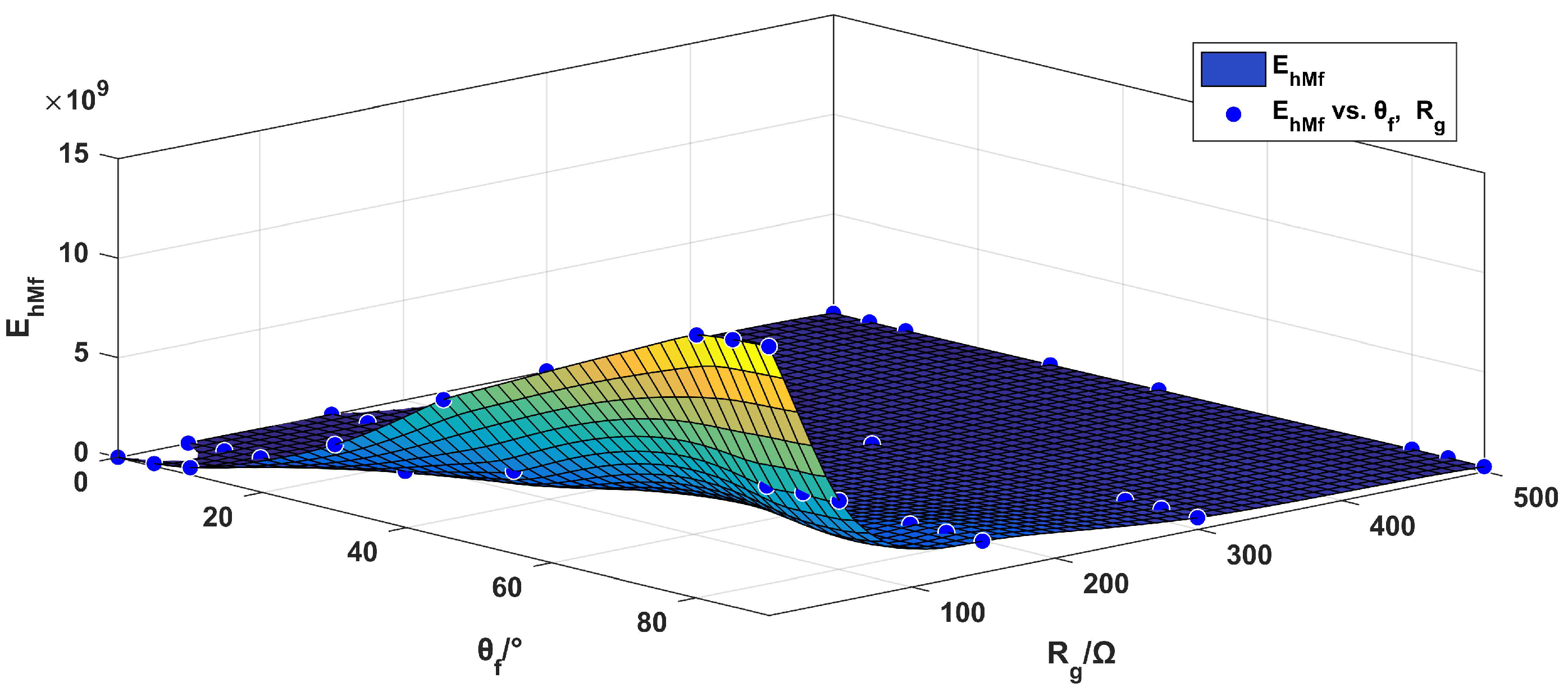
A 500 kV EHV transmission line system as shown in Figure 5 is established in ATPdraw 6.0, and the model parameters refer to the 500 kV Pingwu line parameters of Central China Power Grid. Line PM, line MN and line NQ are 180 km, 172 km and 170 km respectively, and the system frequency is 50 Hz. The line parameters are as follows: positive-sequence reactance, impedance, and capacitance are = 0.2783 /km, = 0.027 /km, = 0.0127 F/km; and zero-sequence reactance, impedance, and capacitance are = 0.6494 /km, = 0.1948 /km, and = 0.009 F/km. Parameters of wave arrestor = 2 mH, = 0.338 mH, = 528 pF, = 3125 pF, = 800 ; the stray capacitance on both sides of the bus is 0.01 μF.In this paper, fault points are set at the point of line MN, point of line NQ, and point of line PM, respectively. The faults in and out of the region with fault angles of 0°, 5°, 10°, 30°, 45°, 80°, 85°, and 90°, and transition resistances of 1 , 50 , 150 , 300 , and 500 are studied. Limited to the space below, only the simulation data of phase A fault are listed.According to the fault simulation data of the point, the data graph of can be obtained, as shown in Figure 6.
4.1. Fault Situation in the Area
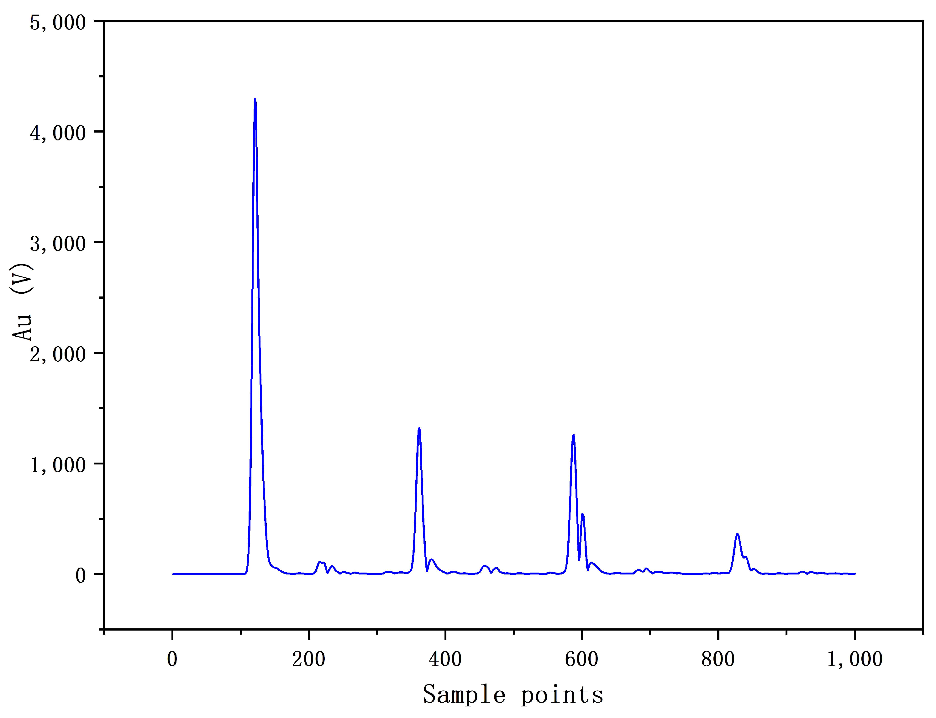
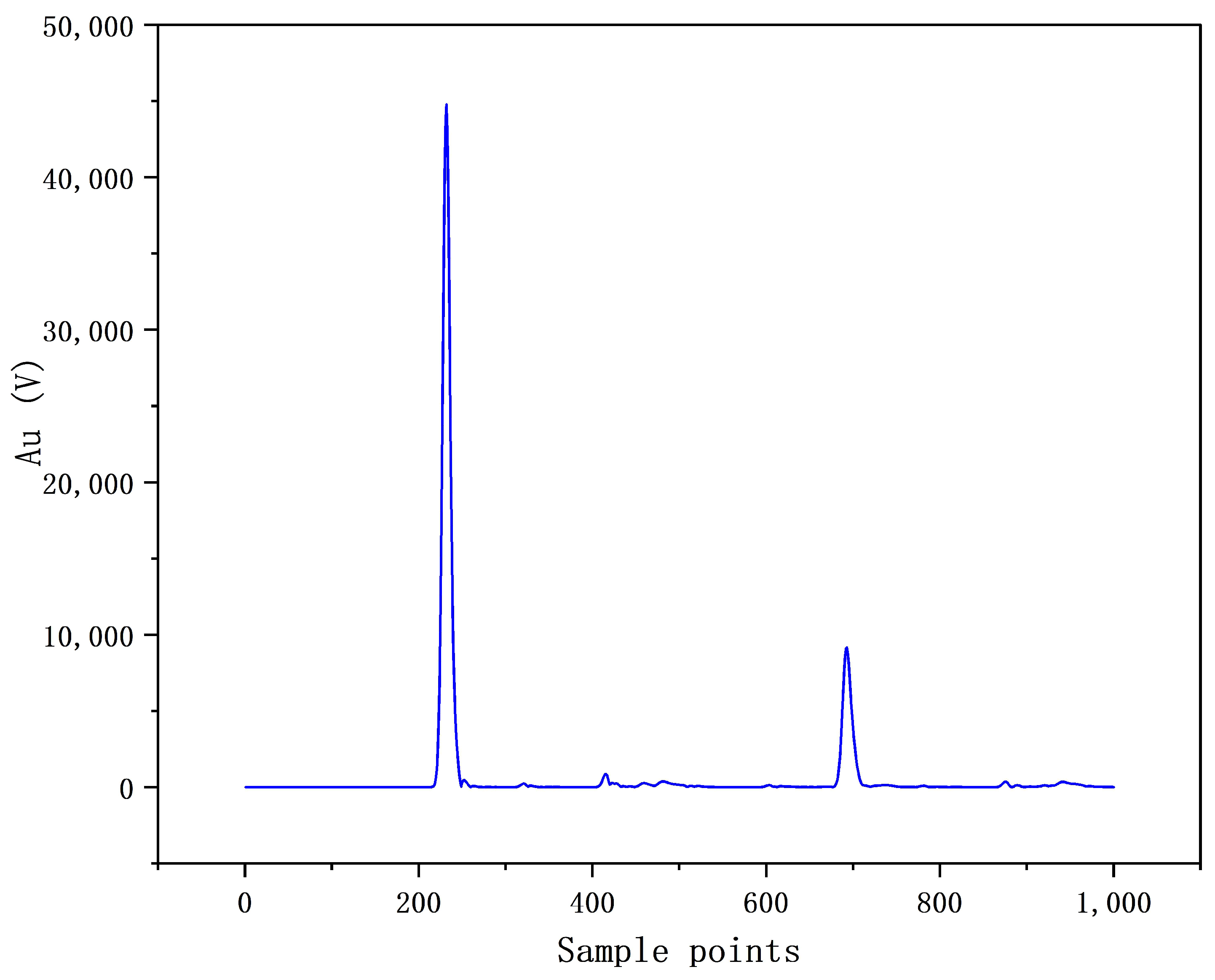
Figure 7 shows the voltage -mode collected at when the fault resistance is 1 and the initial fault angle is 0 after S-transform. As can be seen from the figure, the traveling wave arrives at the protection device is the 232nd point of the time sampling point.
The data of fault at point (4 km from N point) are shown in Table 2. After analyzing the range of data values, it is concluded that when an intra-area fault occurs on the line, the range of fault characteristic is between 0.4 and 1.3. The maximum value of occurs when the initial fault angle is 0°, and the minimum value occurs when the initial fault angle is 90°, and in the case of a fixed initial fault angle, the value of increases with the increase in the transition resistor resistance value. In order to improve the reliability of the protection criterion, it is necessary to leave enough margin to set the value of the fault characteristic quantity between 0.1 and 1.5 when the fault occurs in the line area.
4.2. Fault Conditions Outside the Protected Line
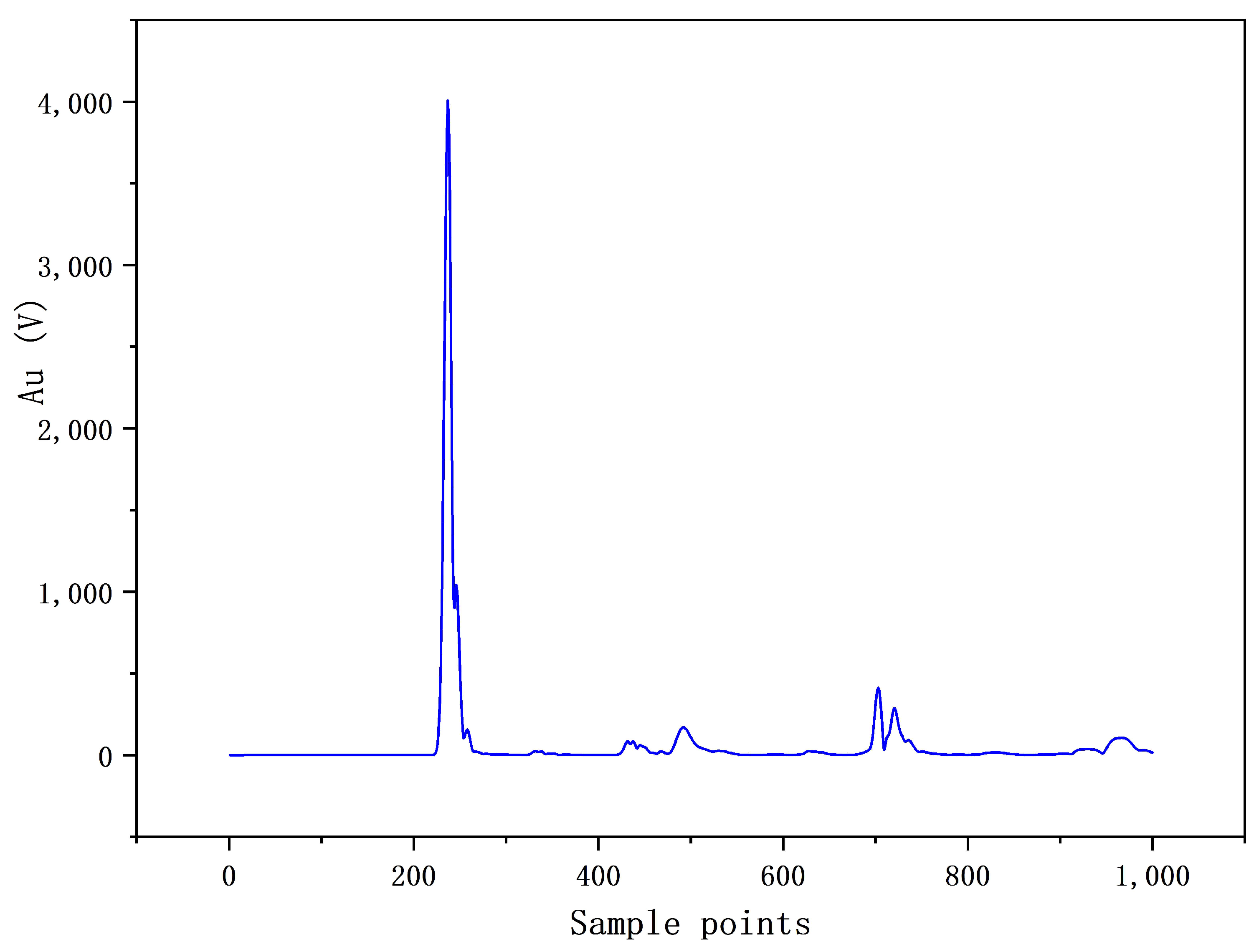
Figure 8 shows voltage -mode collected at . As can be seen from the figure, the time is the 237th point of the time sampling point.
Figure 9 shows the voltage mode collected at . As can be seen from the figure, the time is the 122nd point of the time sampling point.
The data of points (4 km or 166 km from N terminal) and (4 km or 176 km from M terminal) and their faults are shown in Table 3 and Table 4. After analyzing the range of data values, it is concluded that the fault characteristic after normalization is small, greater than 0 but far less than 0.1. The order of magnitude is mainly concentrated in . As can be seen in Table 3, the maximum value of the positive out-of-area fault is about 0.01, and the minimum value occurs in the case of the positive out-of-area fault at the point of the fault that is far away from the protected line, at which time the initial angle of the fault is 0°. As can be seen from Table 4, the maximum value is about 0.01 for reverse-direction out-of-area faults, and the minimum value also occurs in the case of forward direction out-of-area faults at fault points farther away from the protected line, when the initial angle of fault is 0°. Comparing the data in Table 3 and Table 4 with Table 2, it can be seen that there is no numerical overlapping between the fault characteristic quantity after the calculation of in-area faults and out-of-area faults, and the numerical difference is large, with a difference of about 40 times, which is able to carry out the fault discrimination very well.
4.3. Criterion Establishment
From the comparative analysis of the above data of each fault condition, the fault characteristic quantity satisfies when it is an internal fault; while it is an external fault, the fault characteristic quantity satisfies .
Therefore, the significant difference of fault characteristics can be used for criterion setting. When , it is judged as an in-zone fault; in other cases, it is judged as an out-of-zone fault.
5. Conclusions
In order to overcome the defects of the low reliability of the traditional travelling wave, this paper investigates the voltage travelling wave as a fault component and constructs an S-transform based boundary protection considering fault factors. The high-frequency components in the resistive band of the trap are extracted by using the S-transform, and then the resulting S-transform modulus is integrated with the continuous amplitude to derive the voltage travelling wave energy. At the same time, a model is constructed to normalize the voltage travelling wave transient energy according to the initial angle of fault and transition resistance. By normalizing the voltage travelling wave energy, the normalized fault characteristic quantities are derived as the protection criterion, so as to eliminate the influence of fault factors on the protection reliability as far as possible. The energy data before normalization shows that the fault factor has a great influence on the reliability of the protection, and the in-zone and out-of-zone energies are seriously overlapped, and the probability of misjudgement is as high as 85%. After normalization, there is no numerical overlapping of the normalized fault characteristic quantities during in-zone and out-of-zone faults. There is a significant difference between the normalized fault characteristic quantities for in-zone and out-of-zone faults. The ranges from 0.1 to 1.5 in the case of in-zone faults, and from to in the case of out-of-zone faults, with a difference of about 40 times in the case of in-zone and out-of-zone faults. A criterion constructed using the normalized fault characteristics can reliably discriminate between in-of-are faults and out-of-area faults. and the protection is easy to set, with low misjudgment probability and high sensitivity. Through simulation, the criterion is reasonable and has enough sensitivity.
Author Contributions
Z.G. and J.H.: Methodology, Software, Writing. Y.D.: Writing. Q.H., Y.L. and Z.H.: Review, Editing. All authors have read and agreed to the published version of the manuscript.
Funding
This research was funded by the National Natural Science Foundation of China, grant number 52067005; and the Guangxi Natural Science Foundation, grant number 2021GXNSFAA220061.
Data Availability Statement
Data are contained within the article.
Conflicts of Interest
The authors declare no conflicts of interest.
References
- Mehmed-Hamza, M.; Stanchev, P. Sensitivity and Selectivity of Time Overcurrent Relay Protection in Medium Voltage Power Lines. In Proceedings of the 2020 7th International Conference on Energy Efficiency and Agricultural Engineering (EE&AE), Ruse, Bulgaria, 12–14 November 2020; IEEE: Ruse, Bulgaria, 2020; pp. 1–4. [Google Scholar]
- Ghosh, S.; Kedarisetty, S.; Ghosh, D.; Mohanta, D.K. Failure Scenarios of Power System Protection. In Proceedings of the 2021 5th International Conference on System Reliability and Safety (ICSRS), Palermo, Italy, 24–26 November 2021; IEEE: Palermo, Italy, 2021; pp. 1–5. [Google Scholar]
- Hosseini, S.A. Analysis of Substation Protection System Failures and Reliability. In Proceedings of the 2020 15th International Conference on Protection and Automation of Power Systems (IPAPS), Shiraz, Iran, 30–31 December 2020; IEEE: Shiraz, Iran, 2020; pp. 74–79. [Google Scholar]
- Yu, D.K. A Research of Operation Stability of Overhead Transmission Lines’ Relay Protection Algorithms, Which are Based on Travelling Wave Principle. In Proceedings of the 2020 3rd International Youth Scientific and Technical Conference on Relay Protection and Automation (RPA), Moscow, Russia, 22–23 October 2020; IEEE: Moscow, Russia, 2020; pp. 1–21. [Google Scholar]
- Han, Y.; Ma, R.; Li, T.; Zeng, W.; Liu, Y.; Wang, Y.; Guo, C.; Liao, J. Fault Detection and Zonal Protection Strategy of Multi-Voltage Level DC Grid Based on Fault Traveling Wave Characteristic Extraction. Electronics 2023, 12, 1764. [Google Scholar] [CrossRef]
- Wang, S.; Xuan, X.; Wen, M.; Qi, X.; Dong, X.; Li, B. The Research and Development of the High-Speed Transmission Line Protection Based on the Transient Information. In Proceedings of the 2019 IEEE 8th International Conference on Advanced Power System Automation and Protection (APAP), Xi’an, China, 21–24 October 2019; IEEE: Xi’an, China, 2019; pp. 883–887. [Google Scholar]
- Lima, J.R.; Costa, F.B.; Lopes, F.V. Two-terminal traveling-wave-based non-homogeneous transmission-line protection. Electr. Power Syst. Res. 2023, 223, 109622. [Google Scholar] [CrossRef]
- Hu, J.; Wang, Z.; Lan, Y.; Hao, W.; Zhang, Y. Wavelet Energy Entropy-based Transient Protection for EHV AC Transmission Line. J. N. China Electr. Power Univ. (Nat. Sci. Ed.) 2019, 46, 10–18. [Google Scholar]
- Zheng, T.; Song, X. Fast Protection Scheme for AC Transmission Lines Based on Ratio of High and Low Frequency Energy of Transient Traveling Waves. Power Syst. Technol. 2022, 46, 4616–4624. [Google Scholar]
- Yang, R.; Chen, L. A New Principle of Busbar Protection Based on S-transform Current Phase Comparison. Electr. Eng. Mater. 2019, 2, 34–42. [Google Scholar]
- dos Santos, A.; de Barros, M.T.C. Comparative Analysis of Busbar Protection Architectures. IEEE Trans. Power Deliv. 2016, 31, 254–261. [Google Scholar] [CrossRef]
- Wu, H.; Dong, X.; Ye, R. A new algorithm for busbar protection based on the comparison of initial traveling wave power. IEEJ Trans. Electr. Electron. Eng. 2019, 14, 520–533. [Google Scholar] [CrossRef]
- Deng, F.; Zu, Y.; Huang, Y. Research on Single-ended Fault Location Method Based on the Dominant Frequency Component of Traveling Wave Full-waveform. Proc. CSEE 2021, 41, 2156–2167. [Google Scholar]
- Rodriguez-Herrejon, J.; Reyes-Archundia, E.; Gutierrez-Gnecchi, J.A.; Olivares-Rojas, J.; Méndez-Patiño, A. Analysis by Traveling Waves for a Protection Scheme of Transmission Lines with a UPFC. IEEE Lat. Am. Trans. 2024, 22, 46–54. [Google Scholar] [CrossRef]
- Kong, H.; Cong, W.; Zhang, H.; Qiu, J.; Chen, M.; Wei, Z. New Protection Method for High-Voltage Transmission Lines Based on Traveling Wave Energy Comparison. In Proceedings of the 2021 IEEE IAS Industrial and Commercial Power System Asia (IEEE I&CPS Asia 2021), Chengdu, China, 18–21 July 2021; IEEE: New York, NY, USA, 2021; pp. 1115–1120. [Google Scholar]
- Nayak, K.; Jena, S.; Pradhan, A.K. Travelling Wave Based Directional Relaying without Using Voltage Transients. IEEE Trans. Power Deliv. 2021, 36, 3274–3277. [Google Scholar] [CrossRef]
- Wang, H.; Li, X.; Dong, X.; Jiang, X. A Backup Protection Based on Compensated Voltage for Transmission Lines Connected to Wind Power Plants. Electronics 2024, 13, 743. [Google Scholar] [CrossRef]
- Li, X.; Ding, X.; Shu, H.; Na, A.N. A fault identification method of an AC transmission line based on a multifractal spectrum. Power Syst. Prot. Control 2021, 49, 1–10. [Google Scholar]
- Zeng, X.; Zhang, Y.; Wu, Z. HHT based non-unit transmission line protection using traveling wave. In Proceedings of the 2009 IEEE Power & Energy Society General Meeting, Calgary, AB, Canada, 26–30 July 2009; IEEE: Calgary, AB, Canada, 2009; pp. 1–5. [Google Scholar]
- Li, X.P.; He, Z.Y.; Wu, X.; Lin, S. Ultra High Speed Directional Element Based on Amplitude Comparison Using S-transform Energy Relative Entropy. Autom. Electr. Power Syst. 2014, 38, 113–117. [Google Scholar]
- Ghashghaei, S.; Akhbari, M. Transmission line fault distance and direction estimation using artificial neural network. Int. J. Eng. Sci. Technol. 2011, 3, 110–121. [Google Scholar]
- Xu, F.; Dong, X.; Wang, B.; Shi, S. Combined single-end fault location method of transmission line and its experiments. Electr. Power Autom. Equip. 2014, 34, 37–42. [Google Scholar]
- Li, Y.; Zhang, T.; Wen, A. A new location method for UHV AC transmission lines with high resistance faults based on single terminal volume. Power Syst. Prot. Control 2020, 48, 27–33. [Google Scholar] [CrossRef]
- Cong, W.; Ma, Y.; Cheng, X.; Qiu, S.; Wang, G.; Yi, G.; Zhang, L. Transition resistance calculation based on time-domain signals of two terminals. Electr. Power Autom. Equip. 2013, 33, 63–67. [Google Scholar]
- Yu, K.; Mao, Y.; Li., Y.; Zeng, X.; Xie, L. VMD-S Traveling Wave Signal Extraction Method Under Strong Noise. In Proceedings of the 2018 China International Conference on Electricity Distribution (CICED), Tianjin, China, 17–19 September 2018; IEEE: Tianjin, China, 2018; pp. 1739–1743. [Google Scholar]
Figure 1.
Schematic diagram of wave arrester.

Figure 2.
Structure diagram of AC transmission line system.

Figure 3.
Double-ended single-phase transmission system.
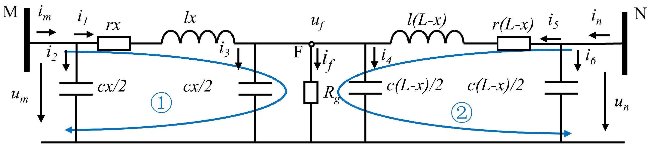
Figure 4.
Composite mode network of single-phase grounding short circuit through transistors.

Figure 5.
500 kV simulation system model.

Figure 6.
three-dimensional diagram.

Figure 7.
Amplitude distribution of voltage mode after S-transform.

Figure 8.
Amplitude distribution of voltage mode after S-transform.

Figure 9.
Amplitude distribution of voltage mode after S-transform.

Table 1.
The energy value of voltage mode under different fault factors.
| 1 | 50 | 150 | 300 | 500 | |
|---|---|---|---|---|---|
| Internal faults (4 km away from M) | |||||
| 0 | 11.4000 | 4.28500 | 1.34400 | 0.48960 | 0.20980 |
| 2 | 258.000 | 96.5500 | 30.2800 | 11.0300 | 4.72600 |
| 5 | 1269.00 | 475.000 | 147.900 | 63.8300 | 27.3500 |
| 10 | 3581.00 | 1339.00 | 418.600 | 152.100 | 65.1000 |
| 30 | 32,800.0 | 12,270.0 | 3835.00 | 1393.00 | 596.400 |
| 45 | 6872.00 | 25,710.0 | 8036.00 | 2920.00 | 1250.00 |
| 80 | 131,200 | 49,100.0 | 15,340.0 | 5574.00 | 2386.00 |
| 85 | 134,100 | 50,180.0 | 15,680.0 | 5700.00 | 2440.00 |
| 90 | 135,000 | 50,480.0 | 15,700.0 | 5735.00 | 2454.00 |
| External faults (4 km away from N) | |||||
| 0 | 0.66920 | 0.34970 | 0.14480 | 0.06169 | 0.02884 |
| 2 | 10.1000 | 5.30500 | 2.19700 | 0.93600 | 0.43760 |
| 5 | 46.7400 | 24.4600 | 10.1300 | 4.31600 | 2.01800 |
| 10 | 120.800 | 63.3400 | 26.3000 | 11.2000 | 5.23600 |
| 30 | 1132.00 | 593.000 | 246.500 | 105.100 | 49.1000 |
| 45 | 2408.00 | 1266.00 | 523.000 | 223.500 | 104.600 |
| 80 | 4579.00 | 2397.00 | 994.900 | 424.000 | 198.100 |
| 85 | 4677.00 | 2454.00 | 1019.00 | 434.100 | 201.900 |
| 90 | 4704.00 | 2468.00 | 1020.00 | 436.300 | 204.000 |
Table 2.
of fault point under different fault conditions.
| 1 | 50 | 150 | 300 | 500 | |
|---|---|---|---|---|---|
| 0 | 0.810 | 0.950 | 1.010 | 1.194 | 1.252 |
| 5 | 0.500 | 0.611 | 0.708 | 0.781 | 0.826 |
| 10 | 0.492 | 0.580 | 0.671 | 0.732 | 0.769 |
| 30 | 0.485 | 0.571 | 0.662 | 0.721 | 0.757 |
| 45 | 0.481 | 0.566 | 0.656 | 0.715 | 0.751 |
| 80 | 0.478 | 0.564 | 0.655 | 0.714 | 0.751 |
| 85 | 0.478 | 0.563 | 0.652 | 0.712 | 0.747 |
| 90 | 0.478 | 0.563 | 0.655 | 0.711 | 0.747 |
Table 3.
of fault point under different fault conditions.
| 1 | 50 | 100 | 300 | 500 | |
|---|---|---|---|---|---|
| 4 km from N terminal | |||||
| 0 | 0.0059 | 0.0081 | 0.0107 | 0.0126 | 0.0137 |
| 5 | 0.0037 | 0.0062 | 0.0071 | 0.0083 | 0.0090 |
| 10 | 0.0036 | 0.0050 | 0.0067 | 0.0078 | 0.0085 |
| 30 | 0.0036 | 0.0050 | 0.0067 | 0.0078 | 0.0085 |
| 45 | 0.0035 | 0.0049 | 0.0065 | 0.0076 | 0.0084 |
| 80 | 0.0035 | 0.0049 | 0.0065 | 0.0076 | 0.0083 |
| 85 | 0.0035 | 0.0049 | 0.0065 | 0.0076 | 0.0083 |
| 90 | 0.0035 | 0.0049 | 0.0065 | 0.0076 | 0.0083 |
| 166 km from N terminal | |||||
| 0 | 0.00007 | 0.0001 | 0.0001 | 0.0002 | 0.0002 |
| 5 | 0.0025 | 0.0037 | 0.0050 | 0.0059 | 0.0066 |
| 10 | 0.0028 | 0.0042 | 0.0058 | 0.0069 | 0.0076 |
| 30 | 0.0030 | 0.0044 | 0.0060 | 0.0071 | 0.0079 |
| 45 | 0.0031 | 0.0046 | 0.0063 | 0.0075 | 0.0083 |
| 80 | 0.0031 | 0.0047 | 0.0064 | 0.0076 | 0.0084 |
| 85 | 0.0031 | 0.0047 | 0.0064 | 0.0077 | 0.0084 |
| 90 | 0.0031 | 0.0047 | 0.0064 | 0.0077 | 0.0084 |
Table 4.
of fault point under different fault conditions.
| 1 | 50 | 100 | 300 | 500 | |
|---|---|---|---|---|---|
| 4 km from M terminal | |||||
| 0 | 0.0042 | 0.0058 | 0.0073 | 0.0084 | 0.0091 |
| 5 | 0.0042 | 0.0058 | 0.0074 | 0.0086 | 0.0093 |
| 10 | 0.0043 | 0.0058 | 0.0075 | 0.0087 | 0.0094 |
| 30 | 0.0043 | 0.0058 | 0.0075 | 0.0087 | 0.0095 |
| 45 | 0.0043 | 0.0058 | 0.0075 | 0.0087 | 0.0096 |
| 80 | 0.0043 | 0.0058 | 0.0075 | 0.0087 | 0.0096 |
| 85 | 0.0043 | 0.0058 | 0.0075 | 0.0087 | 0.0096 |
| 90 | 0.0043 | 0.0058 | 0.0073 | 0.0087 | 0.0095 |
| 176 km from M terminal | |||||
| 0 | 0.0003 | 0.0005 | 0.0006 | 0.0008 | 0.0008 |
| 5 | 0.0052 | 0.0073 | 0.0101 | 0.0119 | 0.0131 |
| 10 | 0.0057 | 0.0082 | 0.0111 | 0.0130 | 0.0142 |
| 30 | 0.0059 | 0.0084 | 0.0115 | 0.0136 | 0.0148 |
| 45 | 0.0061 | 0.0086 | 0.0118 | 0.0139 | 0.0152 |
| 80 | 0.0057 | 0.0082 | 0.0111 | 0.0130 | 0.0142 |
| 85 | 0.0048 | 0.0072 | 0.0099 | 0.0118 | 0.0130 |
| 90 | 0.0048 | 0.0072 | 0.0100 | 0.0118 | 0.0130 |
Disclaimer/Publisher’s Note: The statements, opinions and data contained in all publications are solely those of the individual author(s) and contributor(s) and not of MDPI and/or the editor(s). MDPI and/or the editor(s) disclaim responsibility for any injury to people or property resulting from any ideas, methods, instructions or products referred to in the content. |
© 2024 by the authors. Licensee MDPI, Basel, Switzerland. This article is an open access article distributed under the terms and conditions of the Creative Commons Attribution (CC BY) license (https://creativecommons.org/licenses/by/4.0/).
Share and Cite
MDPI and ACS Style
Guo, Z.; Huang, J.; Deng, Y.; Huang, Q.; Luo, Y.; Huang, Z. Boundary Protection Based on S-Transform Considering Fault Factors. Electronics 2024, 13, 1464. https://doi.org/10.3390/electronics13081464
AMA Style
Guo Z, Huang J, Deng Y, Huang Q, Luo Y, Huang Z. Boundary Protection Based on S-Transform Considering Fault Factors. Electronics. 2024; 13(8):1464. https://doi.org/10.3390/electronics13081464
Chicago/Turabian StyleGuo, Zhenwei, Jiemei Huang, Yingcai Deng, Qian Huang, Yi Luo, and Zebo Huang. 2024. "Boundary Protection Based on S-Transform Considering Fault Factors" Electronics 13, no. 8: 1464. https://doi.org/10.3390/electronics13081464
Note that from the first issue of 2016, this journal uses article numbers instead of page numbers. See further details here.