Abstract
This article introduces a new MfEIT UDESC Mark I system, which consists of a 32-electrode setup featuring a modified Howland current source, low cost, portability, and non-radiation. The system is capable of reconstructing electrical conductivity tomographic images at a rate of 30.624 frames per second, taking about 5 min for imaging. The current source employs a 0.5 mA adjacent current application pattern with frequencies ranging from 10 kHz to 1 MHz. This article outlines the hardware, firmware, and software design specifications, which include the design of the current source, calibration procedures, and image reconstruction process. Tomographic images of conductivity were reconstructed in ex vivo healthy pig lungs and those with pneumonia, as a proof of concept for future applications in live pigs. The high spectral power density, combined with real-time system calibration provides clinical advantages in veterinary medicine. The goal is to identify lung areas affected by Mycoplasma hyopneumoniae in pigs through the analysis of electrical conductivity difference, offering a valuable tool to assist veterinarians to obtain images of respiratory diseases. The modified reconstruction method GREIT (EIDORS) was evaluated with experimental data and was compared with the Gauss–Newton and Total Variation methods, where GREIT 2D proved to be superior.
1. Introduction
Multifrequency Electrical Impedance Tomography (MfEIT) generates low spatial resolution images of the electrical conductivity of pathological tissues in the lungs and hearts of patients in Intensive Care Units (ICUs). These images, when integrated with mechanical ventilation systems, aid in the effective management of patients, helping to avoid excessive ventilation that could lead to fatalities. Both monofrequency and Multifrequency Electrical Impedance Tomography techniques have been developed since the 1980s and serve various applications in medicine. These include monitoring and imaging in cases of hospitalization due to SARS-CoV-2 [1,2,3], acute respiratory distress syndrome (SARS) [4], lung pathologies using artificial intelligence [5], lung cancer [6], lung embolism [7], breast cancer imaging [8,9], prostate tumors [10], tumor detection [11], and emphysema [12]. MfEIT has also been used in conjunction with other imaging modalities, such as magnetic resonance imaging, magnetic induction tomography, and computed tomography, to enhance the speed and quality of image acquisition.
MfEIT applies low-intensity, high-frequency electrical currents to a patient’s chest via a 32-electrode strap. This results in a matrix of potential differences at each applied point. This matrix is then processed with optimization techniques and reconstruction software to produce two-dimensional images of objects under tests [13]. These images can be used alongside other CT modalities and mechanical ventilators for diagnosing conditions like SARS, pulmonary emphysema, and pneumonia, as well as for detecting fluid accumulation in the lungs. Conductivity and permittivity variations linked to pulmonary pathologies can be visualized using specialized hardware, firmware, and algorithms. When tissue is subjected to a low-amplitude, high-frequency alternating current, an electrical potential is generated in the conductive volume. The current injection occurs between two adjacent electrodes, and the voltage measurement is taken between two other electrodes, which may or may not be adjacent. Various patterns, such as adjacent [14], diametrical [15], transversal [16], trigonometric [17], and sinusoidal [18], can be used for current injection and voltage measurements. In the adjacent pattern, one can opt to “skip” one or two electrodes when applying electric current to minimize noise in the measurement system. For example, an alternating current could be injected between electrodes 1 and 2, with subsequent potential measurements starting from electrode 3, proceeding between electrodes 3 and 4, then 4 and 5, and so on.
The objective of MfEIT is to measure the properties of these subjects and visualize them through imaging across a cross-section of a tank. A reference electrode must be connected to a central point to ensure that all measurements from different electrode pairs refer to the same electrical potential [19].
EIT distinguishes itself from other tomographic imaging techniques because it does not use ionizing radiation, enhancing patient safety [20]. This makes it suitable for treating neoplasms and managing mechanical ventilation in ICU beds through an electrode belt attached to the patient’s body [21,22]. However, the distribution of conductivities or permittivities within an organ creates an inverse problem that is ill-posed or rank-deficient. The challenge in MfEIT systems is to optimize and test algorithms capable of solving this problem satisfactorily without losing essential information in the images.
Different clinical applications are possible primarily because there are distinct differences between healthy and pathological tissues, such as tumor tissues. Tumor tissues exhibit higher permittivity and conductivity values compared to normal tissues due to higher water content and sodium concentrations, along with different electrochemical properties in their cell membranes [23]. Biological tissues exhibit varying conductivity, permittivity, and permeability values at radio frequencies [24].
Visualization of lung activity through EIT is feasible because an empty lung has electrical resistance magnitudes twice as high as an inflated lung. Tissue anomalies also alter the regions in which they are present; for example, impedance is lower in the case of a tumor and resistance increases in the case of a pneumothorax (air pocket between the lung and the pleura) [25].
With the magnitude and phase values obtained using the MfEIT system and distributed over a frequency spectrum, the electrical conductivity of the lung becomes visible for diagnostic purposes [26]. The direct problem in MfEIT involves obtaining voltage measurements from the analyzed organ, while the inverse problem focuses on reconstructing the internal conductivity distribution of biological tissues from the acquired potential values [27]. However, there is a consensus in the literature about the methodological limitations of using a priori information for image retrieval and optimization in EIT, aiming at medical diagnosis.
Currently, two image reconstruction techniques are prominent in EIT: static or absolute images [28], and dynamic [29], differential [30], or time-difference images [31]. Monofrequency EIT produces static or absolute images with low precision and therefore cannot detect water or blood in the lungs, for example [32]. Multifrequency EIT generates dynamic or differential images with more defined contours, resulting in a more realistic image [33]. Differential images are constructed using the magnitude or phase differences between data obtained at specific frequency points [30]. Despite over four decades of optimizations and innovations in techniques for solving inverse problems in EIT systems, MfEIT images still suffer from low resolution [34]. The reconstruction process is often slow or inconclusive when compared to other available tomography scans, mainly because the electrode belt moves on the human body and may not capture some internal signals effectively.
In some countries, EIT techniques are used in veterinary medicine. There are, on average, 36 articles and one book chapter published so far, but one application has been made in Brazil.
Most research on animals has utilized the BB2/BBVet tomograph (Sentec, Landquart, Switzerland), and the Pioneer (Sentec, Landquart, Switzerland), both containing 32 electrodes [35].
In 2009, Fagerberg et al. conducted a study to assess pulmonary perfusion over a wide range of cardiac output in anesthetized, mechanically ventilated pigs, using EIT for real-time visualization. The belt contained 16 electrodes arranged at the thorax’s mid-level to generate images of pulsatile systolic changes in impedance synchronized with the pulse [36].
In 2012, Schramel et al. worked with pregnant Shetland ponies using EIT to monitor breathing in these animals. The ventilation process changes during pregnancy and returns to normal shortly after birth. Repeated EIT measurements were taken on conscious, standing animals to visualize thoracic images during breathing [37].
Ferrario et al. (2012) used CT images to develop an algorithm for automatic detection of lung and heart regions in a temporal series of EIT images. The algorithm was validated on a dataset of EIT and CT data from pig organs, demonstrating its ability to reconstruct relevant impedance changes in their anatomical locations by relying only on the thoracic boundary geometry and electrode positions [38].
A portable digital EIT system with eight electrodes was evaluated in 2014 by Ayati et al. for detecting hematomas, using phantoms and sheep models. Changes in phantom conductivity were detected, with anomalies inserted in the center and near the edge of the container. In the sheep model, bleeding rate was monitored while a conductivity solution mimicking blood was injected. EIT images were reconstructed for different injection volumes in phantoms, and using sheep experiment images with simulated hematomas, it was possible to detect the hematomas and their locations [39].
Also in 2014, Moens et al. used EIT to investigate the physiology of lung collapse and recruitment in anesthetized horses. Mechanical ventilation was applied in pressure ventilation mode, and an alveolar recruitment maneuver was performed using a sequence of ascending and descending PEEP (positive end-expiratory pressure) [40].
A new monitoring tool for immobilizing white rhinoceroses with future treatment options using EIT was proposed in 2020 by Mosing et al. They investigated regional ventilation and perfusion measures in immobilized animals in lateral recumbency, aiming to study gas exchange deterioration in rhinoceroses during opioid-induced immobilization [41].
Real-time chest imaging enables the evaluation of ventilation distribution in both anesthetized and conscious animals.
Thoracic EIT was applied to standing and non-sedated horses in 2015, with the assistance of ultrasonic respiratory plethysmography, recording three breaths for analysis. It was concluded that images obtained via EIT provide physiologically useful information, such as sighs, which cannot be easily assessed by other methods [42].
Ambrisko et al. (2017) examined changes in ventilation distribution and regional lung compliances in anesthetized horses during an alveolar recruitment maneuver using EIT. During the alveolar recruitment maneuver, the proportion of tidal volume distributed to the dependent and left lung regions increased due to atelectasis opening. Monitoring dependent lung compliance using EIT may replace PaO2 measurements during the alveolar recruitment maneuver to determine an ideal PEEP [43].
A study investigating the application of EIT to estimate tidal volume by measuring impedance change per breath in healthy anesthetized and mechanically ventilated horses for elective procedures requiring dorsal recumbency was conducted in 2021 by Crivellari et al. [44].
The advantages of EIT over spirometry include the ability to provide continuous breath-to-breath measures without the need for a facial mask or patient intubation. Furthermore, EIT overcomes spirometry limitations in equine applications, as it allows accommodating large tidal volumes without adapting existing equipment or increasing dead space. However, due to not yet being a consolidated technology in veterinary medicine, EIT is a highly expensive monitoring tool for routine clinical anesthesia. It is up to new projects to make the cost of this equipment more accessible to enable its application in animals [45].
The work of Mosing et al. (2017) is a case report describing the use of EIT as a continuous monitoring tool during the general anesthesia of an orangutan with respiratory disease [46].
In 2021, Sacks et al. developed a study describing and comparing variables obtained using EIT in horses with left-sided cardiac volumetric overload, both in compensated and decompensated forms, compared to a group of healthy horses. This overload can result in fluid accumulation in lung tissues, causing changes in ventilation distribution. EIT measurements can be employed as an objective assessment of the impacts of cardiogenic lung disease in these horses [47].
Ambrosio et al. (2017) conducted a study using EIT in dogs to examine the intrapulmonary gas distribution at low and high tidal volumes and investigate whether this is altered by an alveolar recruitment maneuver and positive end-expiratory pressure of 5 cmH2O during anesthesia [48].
A pilot study on thoracic EIT in cattle to identify lung heterogeneity associated with respiratory diseases was developed in 2023 by Brabant et al. Considering that current diagnostic methods are limited, and that there is a lack of crush tests to detect active respiratory diseases in cattle, the use of EIT for real-time visualization of pulmonary ventilation dynamics in these animals was proposed [49].
Wong et al. (2023) studied the use of EIT in anesthetized chickens [50].
This study aims to test and characterize a 32-channel MfEIT system specifically designed for image reconstruction to analyze and characterize lung pathologies in swine with pneumonia.
2. Materials and Methods
This MfEIT system, named UDESC MfEIT Mark I, is derived from the initial project of the Micro-EIT System developed by [51] in 2022. The schematic circuits of UDESC MfEIT Mark I and many results of experiments can be found in Supplementary Materials.
KiCAD version 6.0.7 software [52], available in https://www.kicad.org/blog/2022/07/KiCad-6.0.7-Release/, was used to design all prototype circuits and the electrode board. The prototype comprises an analog interface (Analog Front-End—AFE) with multiplexers, a digital control module, a sanity check board to test the coaxial cables, a switching board containing 32 channels of injectors and sensors, a tank, and the host computer.
The 32 stainless steel electrodes are arranged around a cylindrical acrylic tank, which acts as a test tank. In this tank, phantoms simulating lungs are placed in two liters of 0.9% NaCl solution with a conductivity of 1.3 S/m (20 °C), as indicated in [25].
The host notebook contains the user interface (GUI) and performs image reconstruction of the phantoms using Matlab. It utilizes potential difference data from the 928 measurements made using the MfEIT system. In these measurements, 32 injections and 29 measurements are considered, adhering to an adjacent measurement standard. The circuit acquiring the voltage signals from the tomograph and the switching board is controlled by a unit of the digital system. This unit performs analog-to-digital conversion, generates a 3-mA current signal, selects the gain value, chooses channels, and communicates with the notebook interface. The ADG732 from Analog Devices® (Mouser Electronics, Mansfield, TX, USA) is a 32-channel analog multiplexer with a 4 Ω impedance. It has a single power operation from 1.8 to 5.5 V and a dual power operation from ±2.5 V [53].
2.1. Microcontroller STM32F303ZE-NUCLEO 144
STM32F303ZE-NUCLEO 144 from STMicroelectronics® (Geneva, Switzerland) is a development board featuring a microcontroller (MCU) with the STM32F303ZE model and a printed circuit board specified as the NUCLEO model. This board contains 144 pins for various connections [54]. The MCU’s functions include signal generation, analog-digital conversion, reference generation, and communication with the human–machine interface (HMI).
Relevant parameters of the board include a 32-bit ARM® CORTEX®-M4 processor operating at 72 MHz, with a floating-point unit, multiplication in a single clock cycle, and hardware division. It has up to 512 Kbytes of flash memory and 64 Kbytes of SRAM. The supply voltage ranges from 2.0 to 3.6 V but can reach 5 V via a USB port regulated to 3.3 V. Peripherals include 115 digital I/O pins, 12 DMA channels, four ADCs, 40 channels with conversion speeds of up to 5.1 MHz at maximum resolution, and variable resolutions of 8, 10, and 12 bits, 2 12-bit DACs, a 32.768 kHz crystal oscillator, four operational amplifiers usable as PGAs, 14 timers, and various types of communication including CAN, UART, SPI, and I2C. The STM32F303ZE MCU was programmed in C, using the LL, MBED, and CMSIS libraries. The development tool used was the free version of STM32CubeIDE 1.1.0.1.
The Bioimpedance Front End board comprises the power supply, reference, current meter circuits, current sensor, voltage sensor, output, mux power, MCU interface, two anti-aliasing filters, DAC/Input, and Discrete Interval Binary Sequences (DIBS) [55].
Instrumentation of the prototype employs differential operational amplifiers and anti-aliasing filters to accurately measure the modulus and phase of the electrical impedance, conductivity, or permittivity of biological materials. Consequently, the project aims to analyze the RC charge type of the biological tissues subjected to MfEIT. Typically, a Howland-type current source excites the tissues or phantoms with binary signals through the electrodes, yielding the resulting voltage differences. To minimize noise and distortion in the electrical signals obtained using the MfEIT system, the amplifiers must have a slew rate greater than that in sinusoidal excitation. The maximum rate of change of an operational amplifier’s output voltage is calculated using Equation (1).
where (dvout(t))/dt is the temporal output produced by the excitation circuit of the MfEIT system.
For this purpose, the excitation circuit supplies a sinusoidal current of a given magnitude to the load, using a modified Howland current source [56]. This consists of a voltage-controlled current generator that provides high output impedance and stability to the circuit. The load current must remain independent of the load impedance across the entire frequency range—from 10 kHz to 1 MHz—which is the intended operational range for the tomograph. Given that the system is designed for precise medical diagnoses in Intensive Care Units (ICUs), the quality of the data acquired from measurements of the electrical characteristics of organs must be of the highest possible standard.
CMRR (Common Mode Rejection Ratio) is the ratio between the differential gain (Gd) and the common-mode gain of an amplifier. Ideal differential amplifiers are capable of amplifying only the differential signal while completely rejecting common-mode voltages. To achieve this, the resistors in the circuit must be well-matched. If the resistors are not properly matched, the CMRR value changes. The mathematical expressions to calculate the Common Mode Rejection Ratio (CMRR) in this case are shown in Equations (2) and (3).
where:
- ∆R/R is the resistor matching.
- Gd is the closed-loop gain of the circuit.
The total CMRR (CMRRt), considering a non-ideal amplifier, Equation (2) must include the amplifier CMRR (CMRRampop), shown in Equation (4):
In the voltage source circuit, the input signal should be adjusted for various load values, up to the current injection limit that ensures human safety to avoid burns and accidents. Electrical currents around 20 mA can interfere with a patient’s ability to breathe properly. When the electrical current reaches approximately 80 mA, the patient’s breathing may cease. According to the literature, lethal electrical currents range from 80 mA to 200 mA.
2.2. Howland Current Source
Howland Current Source is a voltage-controlled current generator circuit that provides high output impedance and stable current flow. This circuit is designed to supply a consistent current to the load, independent of the load’s impedance, across a wide frequency range. In medical applications like MfEIT, the Howland Current Source is particularly useful for ensuring accurate and safe measurements. It allows the current to be regulated within the safety limits, especially important in Intensive Care Units (ICUs), where the quality of acquired data is critical.
Differential Howland Current Source has a significantly lower common-mode output compared to the basic single-ended source. To minimize the common-mode voltage generated by the single-ended Howland source and to enhance the voltage tolerance, a differential Howland topology is recommended.
This project utilizes a mirrored differential Howland source based on a differential operational amplifier system, which employs internal common-mode tuning to generate dual outputs of equal magnitude but opposite polarity. Differences between these outputs are directly proportional to the difference between the input voltages, while the common-mode voltage of the outputs is set by the common-mode pin. The source is designed with optimized transconductance to minimize common-mode interference.
Parameters used in this prototype are shown in Table 1.

Table 1.
Howland Differential Mirrored Design Parameters.
These requirements were used to select the op amp and design the Diff-M source for excitation source circuit, as shown in Figure 1.
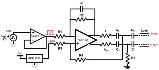
Figure 1.
Excitation Source Circuit (square wave).
Diff-M source, also known as the Modified Differential Enhanced Howland Current Source (MDEHCS-DIF), incorporates operational amplifiers. It is a variant of the original Howland Current Source Differential (HCS-DIF) design, distinguished by the addition of resistor R5.
2.3. AD8132ARZ High Speed Differential Amplifier
AD8132ARZ (Mouser Electronics, Mansfield, TX, USA) is a differential amplifier with a 300 MHz bandwidth, capable of delivering stable unity gain and a high slew rate of 1200 V/µs, making it suitable for generating sine waves at 100 kHz (this value should be verified in practice). It offers high input impedance, a crucial feature for Howland sources, as it minimizes or even eliminates stability issues while maintaining high output impedance. The common-mode pin on the AD8132 is configured at 1.65 V [56].
For the Diff-M [55] current source, the resistors specific to the Diff-M configuration should be calculated using Equations (5) and (6):
Equation (6) represents the common-mode equilibrium condition, which minimizes the output common-mode voltage:
If both conditions are met, the output current is defined using Equation (7):
Equation (7) describes the Howland equilibrium condition, necessary to obtain maximum output impedance.
Any set of resistors satisfying all of Equations (5)–(7) can be used to provide a stable current source.
To reduce the value of rx, the ratio R2 = R1 was selected to be 0.5, which is an attenuation gain that still keeps the AD8132 stable. This is done to increase the maximum load, as large values of rx tend to reduce voltage compliance. The input voltage comes from the input–output ratio of the MCU, which has a maximum amplitude value of 1.65 V (0 to 3.3 V peak-to-peak). To satisfy the output current described in Table 2 the value of rx must be 3.3 kW, as calculated by Equation (7).
Table 2.
Resistance values for the Diff-M current source.
Using the balancing conditions described earlier, the value obtained for the set of resistors is shown in Table 2.
A 0.5 pF negative feedback capacitor, C1, was incorporated into the design to enhance the stability of the modified Howland current source. To isolate the DC component from the biological load, 1 μF capacitors were employed [51].
For generating sine waves, the digital general-purpose input/output (GPIO) pins of the microcontroller were utilized as the input signal. The impedance of these digital pins could potentially disrupt the balance of the modified Howland source. To mitigate this, a voltage buffer using the OPA 2810 IDR [57] amplifier (Mouser Electronics, Mansfield, TX, USA) was implemented to shield the Howland source from the impedance of the GPIO pins.
2.4. OPA 2810 Operational Amplifier
This operational amplifier OPA 2810 offers dual-channel functionality, operates at 27 V, and has high input impedance due to its FET inputs. It also maintains stable unity gain at 105 MHz and achieves high slew rates, specifically 192 Vrms [57]. OPA 2810 parameters [57] are compiled in Table 3.
Table 3.
OPA 2810 Parameters.
2.5. Reference Source—REF2033
A REF2033 reference source from Texas Instruments® (Dallas, TX, USA) was utilized to provide a stable 1.65 V voltage to the positive pin of the Howland current source [58]. This was done to set the differential input to zero. Table 4 describes parameters of the REF2033 reference source.
Table 4.
REF2033 Parameters.
2.6. Electric Potential Measurement Module
This subsection delineates the voltage acquisition and measurement circuit, a key module responsible for capturing voltage differentials across various electrode pairs within the MfEIT system. The module processes signals from the 32 stainless steel electrodes situated within an acrylic tank, eliminating common-mode voltage, amplifying signal amplitude, and filtering out direct current components and high-frequency noise. Subsequently, the conditioned signals are forwarded to the analog-to-digital converter (ADC).
Image reconstruction quality is heavily contingent upon the underlying electronic architecture of the prototype, and thus it varies appreciably across different MfEIT systems. Potential sources of interference compromising image fidelity include measurement noise, cable crosstalk, electrode configuration, current source design and components, high contact impedance, common-mode gain errors, and thermal noise, as well as data acquisition protocols.
To enhance common-mode rejection ratio (CMRR) and confer electromagnetic interference (EMI) immunity, the circuit was designed for fully differential signal operation. This is especially crucial in hospital settings where an array of EMI sources can distort MfEIT measurements, thereby undermining the efficacy of the device in maintaining accurate mechanical ventilation.
Differential measurement techniques augment the system’s linearity, voltage compliance, and signal-to-noise ratio (SNR). The SNR, quantified in decibels (dB), is a critical design consideration for the tomographic measurement system.
Initial development phase of the MfEIT system focused on the input circuit, designed to offer high input impedance while minimizing current leakage. To achieve this, a dual-buffer configuration, as opposed to a differential amplifier, was implemented.
The buffer, based on the OPA2810, offers field-effect transistor (FET) inputs and stable unity gain. To isolate the variable gain amplifier’s (VGA) second-stage direct current voltage, a pair of 2 μF capacitors were deployed in series with the buffer outputs.
A high-pass filter was implemented using capacitors paired with a PGA input resistance of 500 Ω. With a cutoff frequency of 159.15 Hz, approximately 62 times lower than the minimum operational frequency of 10 kHz, the filter effectively mitigates phase errors [51].
Second stage of development in the MfEIT system focuses on the Variable Gain Amplifier (VGA), designed to modulate the amplitude of the measured signal to maximize the resolution for the Analog-to-Digital Converter (ADC). Controlled by one of the microcontroller’s Digital-to-Analog Converter (DAC) channels, the VGA utilizes an AD8338 chip [59] as its core component. This chip operates as a fully differential VGA, executing amplification in current mode. The amplified current is subsequently converted into a differential voltage output via two transimpedance amplifiers.
Common-mode voltage of the circuit is internally set at 1.5 V, necessitating DC blocking via 2 mF capacitors. Differential gain control is achieved through DAC voltage modulation, with gain ranging linearly from 0 dB to 80 dB at a volts-to-dB slope of 12.5 mV/dB. Although the VGA primarily operates in current mode, it also accommodates voltage inputs via its internal 500 Ω resistors.
The final stage in the voltage measurement circuit is the anti-aliasing filter, implemented as a third-order Butterworth multiple-feedback filter (Digi-Key Electronics, Thief River Falls, MN, USA). Employing a fully differential topology, this filter is based on the AD8132 amplifier (Mouser Electronics, Mansfield, TX, USA). It is designed with a cutoff frequency of 1 MHz and a quality factor of 0.707, thereby ensuring a flat response with minimal error at its peak frequency of 100 kHz. Resistor and capacitor values for this filter were determined using the Texas Instruments™ Filter Design Tool. Initially, a single-ended circuit configuration was computed, which was later adapted for full differential operation. The filter output is interfaced with the differential ADC and is equipped with 3.3 V Zener diodes at both outputs, serving as a protective measure for the microcontroller inputs.
2.7. Commutation Stage
Switching Stage Manages Electrode Connections to the Radial Component. To accommodate various EIT protocols, each electrode must be switchable to both the voltage measurement and the data acquisition modules. In this setup, four ADG732BSUZ multiplexers were used. The ADG732BSUZ (Mouser Electronics, Mansfield, TX, USA) is a single CMOS analog multiplexer with 32-to-1 channel configuration. It switches one of the 32 inputs (S1–S32) to a common output, D, as determined by the 5-bit binary address lines A0, A1, A2, A3, and A4 [60]. Its features include a single supply voltage range of 1.8 V to 5.5 V; dual supply operation of ±2.5 V; 4 Ω on-resistance; 30 ns switching time; and inputs compatible with both TTL and CMOS.
ADG732BSUZ has a maximum transmission rate of 33 ns that is the switching time. For an adjacent EIT protocol that excludes measurements on electrode pads, 928 measurements are required, leading to a maximum frame rate of 1 = (928 × 33 ns) = 30.624 frames per second. The using ADG732BSUZ is the reduced speed, particularly in systems utilizing 32 or more electrodes.
2.8. Tank with Exciting Electrodes, Designed Phantoms and Biological Organic Samples
Electrode setup comprises 32 rectangular stainless steel sensors, each measuring 12.5 cm in height and 1.0 cm in width. These are evenly distributed around a cylindrical acrylic tank with dimensions of 10 cm in height and 32 cm in diameter.
Connectivity between the electrode tank and the analog front-end is established through 32 coaxial copper cables. These cables link the electrodes to the use of AD732BSUZ analog multiplexers, facilitating the acquisition of 2D images of the target phantoms, organic samples, and swine lungs throughout image reconstruction software 2D Graz Consensus Reconstruction Algorithm for EIT (GREIT), Total Variation (TV), and One-Step Gauss–Newton (OSGN).
Four hollow phantoms mimicking heart and lung anatomies were fabricated: two from insulating TPU material with a filament diameter of 2.85 mm, and two from conductive ABS with a filament diameter of 1.75 mm. The heart phantom made from conductive ABS stands 12 cm tall, while the lung phantoms in the same material have a height of 27 cm. These conductive phantoms were filled with gelatin and submerged in a NaCl 0.9% solution within the tank, as shown in Figure 2.
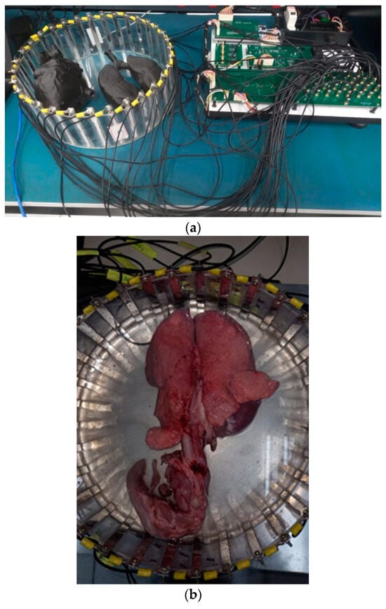
Figure 2.
(a) Tank with phantoms and (b) Tank with healthy swine organs.
Organic samples used in this experiment were potatoes, carrots, apples, and cucumbers, in cylindrical shape, 4.0 cm wide. Glass, metal, and aluminum were also used to characterize the measurement system and image depth.
Samples were placed in a tank with three liters of 0.9% NaCl solution in five different positions, with electrodes marked. The best image reconstruction was in the central position of the vat. Gains were varied from 0 (no gain) to 255 v/v and frequencies from 10 kHz to 1 MHz were varied to characterize the equipment and choose the best parameters for image reconstruction.
2.9. Signal Specification and Measurement Protocol
The equipment was designed to measure the Electrical Impedance Tomography Time Difference (TDEIT) at 10 kHz and the EIT Frequency Difference (FDEIT) at 10 kHz and 1 MHz. To prevent frequency variations caused by parasitic capacitances and other imperfections, the calibrated FDEIT method proposed by Wu et al. [61] was implemented. The frequencies were selected because they fall within the alpha and beta dispersion range, commonly used for tissue characterization [62]. During each scanning cycle, five periods of the voltage response signal were captured for each channel. As the signals were in the form of square waves, the Fast Fourier Transform (FFT) was applied to isolate the magnitude of the fundamental frequency. Only the absolute magnitude of this fundamental frequency was used in signal reconstruction.
The proposed MfEIT system implements the adjacent measurement protocol without measuring the voltage at the current electrodes. This protocol was chosen for its convenience and excellent performance in obtaining images of organic samples, as well as reducing the number of required measurements [61]. The opposite measurement protocol is an additional option that will be implemented in the future, offering a higher field density in the center of the tank and, therefore, better sensitivity to identify variations in central conductivity. With our prototype containing 32 electrodes, the adjacent measurement protocol requires 29 × 32 = 928 measurements. The time for each measurement can be calculated using Equation (8)
where ttotal is the total measurement time, ts is the sampling time, tsw is the switching time, and test is the channel stabilization period.
2.10. Firmawe and Host Computer
MfEIT UDESC Mark I System firmware consists of two codes described in Matlab version 2022a, MathWorks. The first code sets parameters such as port selection, baudrate = 115,200, buffer size = 1000, data bits = 8, stop bits = 1, parity = Odd, and uart delay = 1/1000. It operates with a sampling frequency of 2 × 10⁶ Hz. The user is prompted to choose whether to run the injection and adjacent measurement protocol for collecting voltage measurements between electrodes or to test the channels. Additionally, the user can select the gain value from 0 to 255 v/v and the measurement frequency from 10 kHz to 1 MHz. In this step, measurements of electrode voltages are taken by injecting 0.5 mA of electrical current. A text file with 928,004 points is saved, which will later be used for image reconstruction.
Injection value remains constant in this equipment. Channel testing can be performed if there are any inconsistencies in the measurements. For each frequency, gain, and sample, two measurements should be taken one with a homogeneous sample (without objects or organs inside, only 3.0 L of NaCl) and one with a heterogeneous sample (with an object or organ positioned in a specific location in the tank add 3.0 L of NaCl). Each measurement collection takes about 5 min to obtain.
Second code reads the matrix of 9,280,004 points and transforms it into a matrix of 928 points using an equation based on the first-order harmonic of the two signals (homogeneous and non-homogeneous). Graphs of the fast Fourier transform (FFT) in the time domain and frequency domain are generated, as shown in Figure 3.
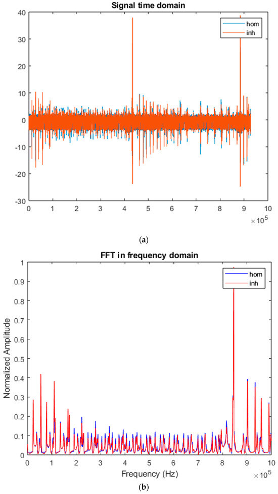
Figure 3.
Examples signal at 50 kHz: (a) FFT in time domain and (b) FFT in frequency domain.
Blue signal represents the homogeneous sample, and the red signal represents the non-homogeneous sample. The third step involves reconstructing the image from these matrices.
2.11. GREIT (EIDORS) for Image Reconstruction and SNR
This work uses EIDORS, version 3.9 [63], for image reconstruction for organic samples. GREIT (Graz Consensus Reconstruction Algorithm for EIT) [64] was modified to adapt the MfEIT UDESC Mark I System.
EIDORS consists of an open-source platform that aims to provide free algorithms for forward modelling and inverse problems solutions in EIT. Netgen, version 4.9.13, is used for EIDORS to create several bidimensional and tridimensional models of varying geometries and sizes.
For comparison, the image reconstruction methods One-Step Gauss–Newton [65] and Total Variation [66] were employed.
In GREIT, the model selected is “cylindrical shape” (32 × 1 electrode belt) with height equal to 2, tank radius equal to 16, and mesh refinement equal to 0.3. The parameter “electrode position” is chosen as 32 electrodes at z = 1 (i.e., one electrode layer only) and “electrode shape” was chosen radius of rectangular electrodes is 0.05, “0” means full electrode model, and mesh refinement is equal to 128. Options chosen were no measurement current and no rotate measurement, following the pattern established by the algorithm.
In this parameter “[fmdl.stimulation,fmdl.meas_select] = mk_stim_patterns”, 32 electrodes were selected, layer, adjacent injection and measurement pattern, and 0.5 mA of injected electrical current.
The creation of the two-dimensional GREIT model utilizes the image size options (opt.imgsz) selected as 64 × 64 pixels; 128 would be the optimal choice, but the processing time becomes excessively high. The value of the noise addition parameter in the image (opt.noise_figure) can be adjusted, in our case, between 0.2 and 0.9. Noise figure values equal to 0.1 or 1.0 result in the image having many unnecessary artifacts. We used the value of 0.3 to 0.45 for most objects whose images were reconstructed. The “opt.distr” parameter for organic sample images was chosen as 1, and for swine lungs, we selected 2. Finally, opt.square_pixels was set to true, as the default for GREIT.
For comparison of images generated using 2D algorithms, the code for the EIDORS Gauss–Newton Solver was chosen, and the creation of the two-dimensional inverse model used “eidors_obj(‘inv_model’, ‘EIT inverse’)” with a background value of 1 and a reconstruction type of “difference.” The hyperparameter value is 2.9 with a Noser prior. The model is “mk_common_model(‘d2c’,32)” with 1024 elements, and the Gauss–Newton solver used was “inv2d.solve = @eidors_default”.
Finally, the Total Variation Solution code was also tested with a hyperparameter value of 0.004, “invtv.solve = @inv_solve_TV_pdipm”, a tolerance of 1 × 10⁻³, and the number of iterations set to 1, 100, 125, and 150. Previously, it was tested with 1, 3, 5, and 25 iterations, showing significantly poorer performance. Other parameters used were “invtv.solve = @inv_solve_TV_pdipm” and “invtv.R_prior = @prior_TV,” which are default settings for the algorithm. Hyperparameter values in OSGN and TV algorithms controls the amount of regularization in the image reconstruction.
The SNR of the images was calculated using the EIDORS function [SNRmean, SE, debug] = calc_image_SNR(imdl, hyperparameter, doPlot). The input and output parameters of this function are explained in reference [67].
The modified codes of the three image reconstruction programs, as well as the remaining codes, can be found in can be found in Supplementary Materials.
2.12. Calibration
In all images, discrepancies between channels were calibrated. The calibration process involved multiplying the data by a calibration factor as shown in Equation (9).
The term error(%) corresponds to the error vector. Additionally, the difference frequencies EIT (FDEIT) images data was subsequently calibrated to mitigate the effects of circuit parasitic components. The calibration method implemented was proposed by Wu [46], who conducted FDEIT measurements on a homogeneous saline sample and used the data vector as a reference, as shown in Equation (10).
It is assumed that the reference saline sample is frequency-invariant, so any detected variation is generated by the circuit itself. Considering that the impedance of the samples is not significantly different from the homogeneous reference, the variations remain constant across all samples. Therefore, by subtracting the reference vector, the circuit error can be eliminated.
3. Results
It is still a proof of concept to use the UDESC Mark I MfEIT in the veterinary field, as multifrequency EIT has never been used in either living or ex vivo animals. In this initial stage, the prototype and software were tested and validated on ex vivo pig lungs. Subsequently, the equipment will be tested with a belt of zinc or stainless-steel electrodes on live animals.
The image reconstruction software used was EIDORS. Initially, we reconstructed the images in the MfEIT UDESC Mark I in EIDORS and, later, we will use deep learning for classification and regression. Each step of the prototype project has been described in the Methodology section. In this section, the characterization of the electrical circuits designed for the tomograph, its electrical performance, will be presented and analyzed, with the aim of validating its possible future applicability in detecting lung pathologies.
MfEIT UDESC Mark I was calibrated at 10 kHz (frequency of the reference image) and at other frequencies without heterogeneous samples inside the tank. The channels were also calibrated based on Matlab codes. To validate this system, several experiments were conducted with conductive and insulating materials over a period of two months in a laboratory at 23 °C. Image reconstruction tests were conducted with apple, potato, carrot, cucumber, banana, glass, and aluminum pieces with various geometries and diverse gains. This allowed for selecting the best gain values, which go up to 50 v/v, adjusting the positions of the elements in the tank, and concluding that larger objects provide images with more faithful contours.
The measurements of potentials were obtained, and images of two domestic swine, lineage of large white, were reconstructed on 9 November 2023. The swine were slaughtered using the UMANA [68] captive bolt stunner, following the gold standard in veterinary care for the humane slaughter of swine. One lung was deemed healthy by the veterinarians overseeing the experiment, while the other showed signs of swine pneumonia. The hearts and trachea were included in the image reconstruction. The protocol of experiment was registered with the Committee on Ethics in Animal Use—CEUA/UDESC, under number 6931201222.
Lungs Swine Images Reconstruction
The size of healthy lungs containing the heart and trachea is 21 cm for the left lung and 17 cm for the right lung. The size of lungs with pathology (plus heart and trachea) is 20 cm for the left lung and 16 cm for the right lung. The central position of the tank was chosen due to the size of the animals’ organs and images of healthy swine lungs and heart versus pneumonia swine lungs at frequencies of 10 kHz, 20 kHz, 30 kHz, 40 kHz, 50 kHz, 90 kHz, 100 kHz, 200 kHz, 300 kHz, 400 kHz, 500 kHz, 900 kHz, and 1 MHz, respectively, were obtained.
Images using GREIT algorithm modified were selected at three frequencies—10 kHz (reference), 200 kHz, and 1 MHz—as shown in Figure 4.
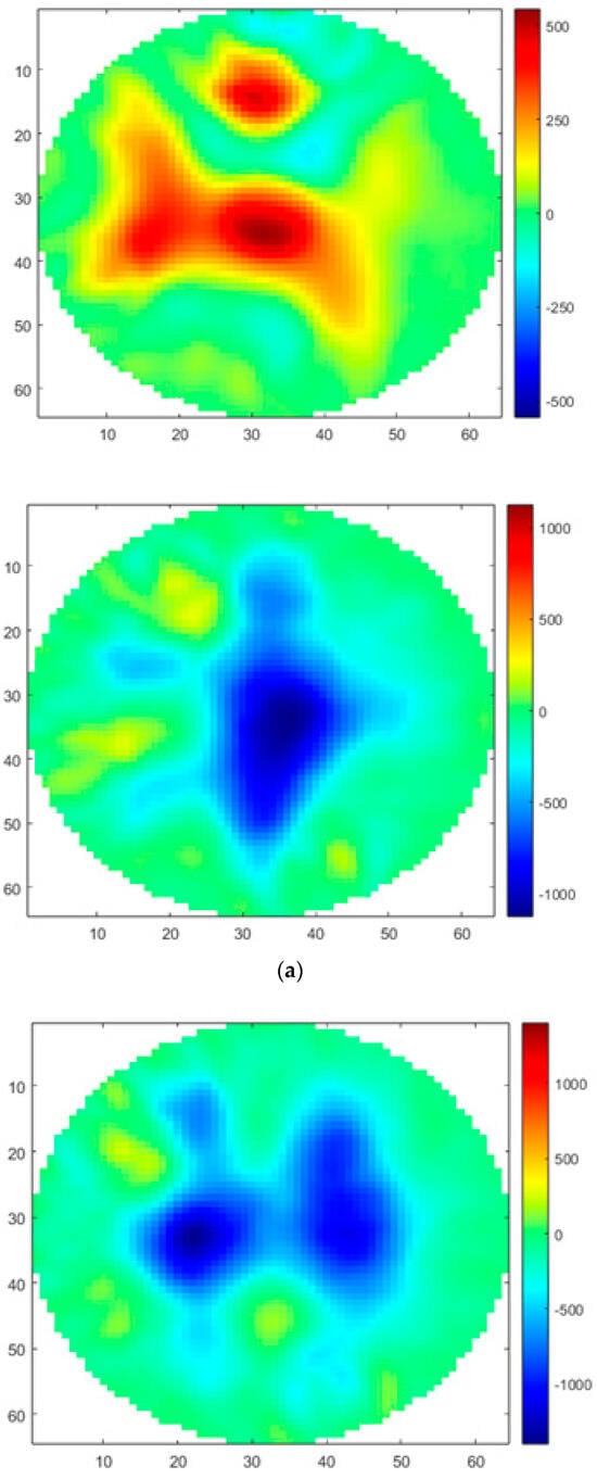
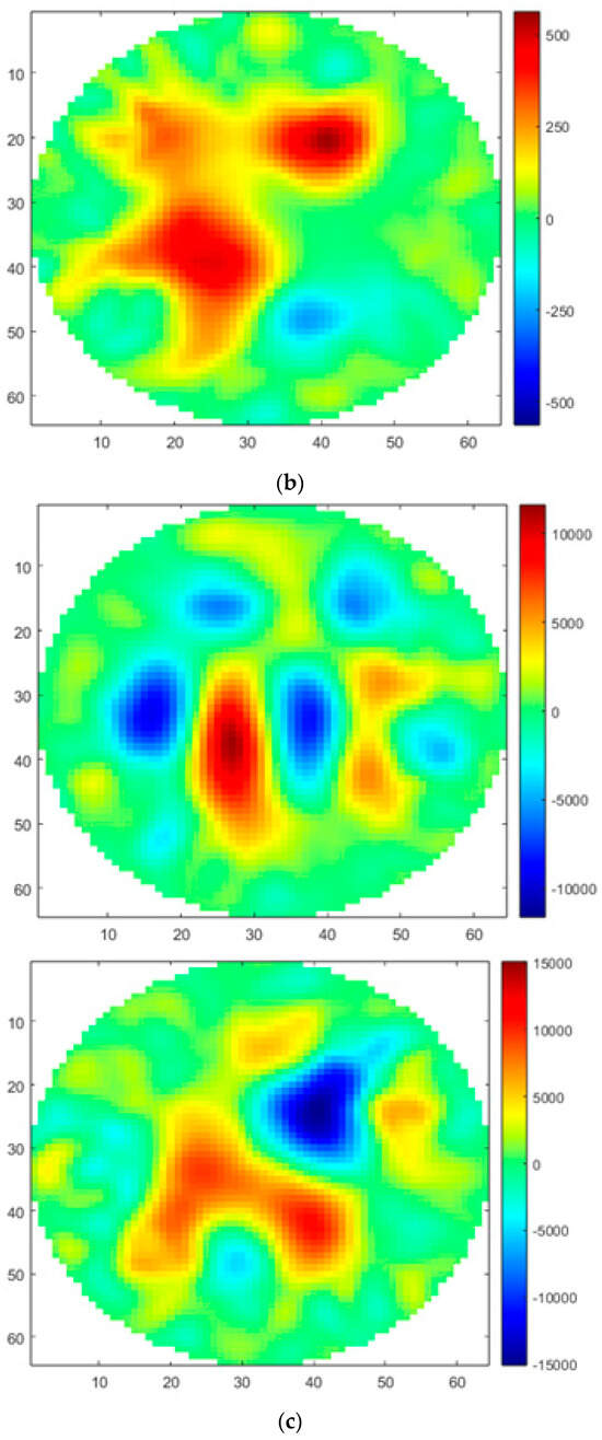
Figure 4.
Sets of reconstructed images of swine lungs without gain, where (a) 10 kHz—up: healthy lungs and down: pathological lungs swine; (b) 200 kHz—up: healthy swine lungs and down: pneumonia swine lungs; (c) 1 MHz—up: healthy swine lungs and down: pneumonia swine lungs.
The images of healthy swine lungs and heart at frequencies of 10 kHz, 20 kHz, 30 kHz, 40 kHz, 50 kHz, 90 kHz, 100 kHz, 200 kHz, 300 kHz, 400 kHz, 500 kHz, 900 kHz, and 1 MHz, respectively, no gain, reconstructed using the Total Variation and One-Step Gauss–Newton algorithms, are shown in Supplementary Materials.
4. Discussion
It is noted that the MfEIT UDESC Mark I System reconstructs tomographic images by varying the contour shapes of the object as the frequency changes and it can be applied to veterinary medicine using a frequency of 200 kHz. It also detects the position of the object inside the tank and displays this displacement in the reconstructed image. The conductivity variation for each pair of lungs and heart, in [S/m], is shown through the color scale and values described in the colorbar, allowing the veterinarian to distinguish the diseased lung.
As this is a preliminary test and validation of the equipment, further future tests on live animals should be conducted, and the results published for discussion.
GREIT algorithm used for image reconstruction exhibits superior performance and resolution compared to the Total Variation (TV) and One-Step Gauss–Newton (OSGN) algorithms [69,70]. The images obtained using the TV and OSGN algorithms were not shown in this article as they were not of useful interest and were only used to select the best algorithm for veterinary use. Anyway, GREIT was the best image reconstruction software tested up to the present moment for the suggested hardware. Performing preprocessing of the potential difference signals will help achieve sharper images with fewer artifacts. This is the next step in this study.
In some frequencies, such as 900 kHz and 1 MHz, it is noted that the GREIT algorithm did not accurately depict the organ positions, nor did it accurately represent their correct geometry. For this reason, it is recommended to use the MfEIT UDESC Mark I system at other frequencies. At 10 kHz and 200 kHz, the images are more faithful to the actual organs.
For organic samples, whose images were not shown in this article to avoid extending the reading, the most difficult place to detect a small object is the center of the tank. One suggestion for future work is to adjust the position in the algorithm as suggested in the literature.
However, for the lungs and hearts of pigs, which are larger organs, this difficulty does not occur.
Hardware limitations also interfere with the quality and accuracy of the reconstructed images. The suggestion is to test the prototype with a current source with an excitation value greater than 0.5 mA. Another idea is to test this system with the opposite measurement standard or by varying the excitation current as the frequency increases.
A stainless-steel grounding plate was used as a reference to avoid artifacts and unwanted interferences in the images, thus enhancing their reliability. However, it is suggested to 3D-print a tank in PLA with two layers using a 3D printer, and to use ring electrodes instead of rectangular electrodes.
From these initial images obtained from the MfEIT UDESC Mark I, the intention is to refine algorithms for the specific case of veterinary medicine, with applications in swine respiratory diseases. Analyzing lung lesions in pig slaughterhouses is crucial for obtaining relevant information about the prevalence of respiratory diseases in pigs [70,71].
Due to limitations in image algorithms, such as bidimensionality, manual adjustment of parameters to obtain the best image, object positioning adjustments in the tank, and the need for post-processing of images with the use of a filter in the initial data treatment, the image quality was reduced. However, except at 1 MHz, changes in conductivity and lung contours are visible at other frequencies. Some artifacts are present but can be avoided by applying the Independent Component Analysis (ICA) technique [72,73,74].
The evaluation of pneumonia in pigs is a key factor in monitoring the health of the animal for slaughter and the quality of meat in slaughterhouses. The normal temperature of a healthy pig, from birth to several months of age, is around 39.2 °C. Currently, pig health diagnosis is carried out through a veterinarian’s visit to pig facilities, where various aspects are observed, such as the condition of the pen and feeders, the condition of each specific animal, analysis of abdominal size, fever measurement, blood tests, PCR, ELISA, vaccine verification, histopathology, and other invasive exams.
In cases of swine pneumonia, extravascular lung water can be determined by assessing the characteristic changes seen in MfEIT. Swine tuberculosis, caused by Mycobacterium tuberculosis, is currently considered rare, with the microorganism Mycobacterium avium being the most common. This contamination occurs through water. The disease causes nodules in the neck lymph nodes, resulting in carcass rejection at the slaughterhouse. In cases of tuberculosis, MfEIT can also be useful in early detection through imaging. In most countries, if neck lesions are detected during post-mortem inspection at the slaughterhouse, the head is rejected, and if lesions are found in the mesenteric lymph nodes that drain the intestine, the viscera are rejected. If the disease is widespread throughout the body, which is rare, there will be total carcass rejection. If small lesions are not detected during inspection, normal meat cooking will destroy the microorganism.
Therefore, the use of MfEIT is suggested for the early detection of respiratory diseases in pigs. The veterinary field lacks this type of equipment, often having only magnetic resonance imaging and X-rays. MfEIT becomes interesting for monitoring lung diseases in pigs due to its portability, low cost, radiation-free nature, and its ability to be used at the bedside in cases of pig hospitalization. EIT can also assist in the diagnosis of African swine fever, where recent outbreaks have occurred mainly in small livestock farms that purchase breeds of unknown origin and have poor hygiene in their facilities. In many locations, producers are not interested in using ASF vaccines on their pigs.
In cases where the abdomen of the pig is enlarged, it is estimated that the pig is infected with Taenia solium. Therefore, MfEIT imaging monitoring prevents the parasite from spreading throughout the body of pig, helping the rural producer diagnose the problem early and carry out appropriate treatment, without affecting the sale of pigs for slaughter and meat consumption. This problem was also detected with MfEIT UDESC Mark I.
5. Conclusions
This work showed the development and validation of an MfEIT system for measuring d.d.p. in 32 electrodes for real-time reconstruction of lung images. Firmware was developed on the Matlab platform for the development board, generating the current excitation signal and acquiring potential differences for each electrode pair in the tank. This firmware processes the data obtained using the prototype and sends it to the host computer. Another Matlab code was developed to filter the signal’s harmonic and reduce the number of acquired points used in the image reconstruction algorithm. The 2D GREIT algorithm was modified and adapted for image reconstruction. The Total Variation and One-Step Gauss–Newton algorithms were also adapted, but they did not show good performance compared to the two-dimensional GREIT.
TPU, PLA, and conductive ABS phantoms were researched and developed for the tests and the ontained results were explained.
The obtained results included bench testing and the reconstruction of conductivity distribution images using the two-dimensional GREIT in conductive (with gelatin inside) and insulating phantoms. The MFEIT reconstructed the phantoms and recognized the conductivity differences. The same occurred with images of organic samples, allowing for setting the optimal object position in the tank and selecting the most appealing gain values according to the desired frequency. The 1 MHz frequency does not reliably reconstruct objects due to the presence of numerous artifacts. The images of pig lungs open up the possibility of using MfEIT equipment in veterinary medicine for the detection of lung diseases, thereby increasing the reliability of the quality of pork for human consumption.
In future works, the development of a belt with 32 electrodes is suggested to apply the MfEIT system to live pigs and study the presence of edema, pneumonia, and other respiratory diseases to detect pathologies in advance of the animal’s slaughter.
Supplementary Materials
The materials and codes was deposited in GitHub: https://github.com/juliagwolff.
Author Contributions
Conceptualization, J.G.B.W. and A.S.P.; methodology, J.G.B.W. and A.S.P.; software, J.G.B.W. and R.K.; validation, J.G.B.W. and R.K.; formal analysis, J.G.B.W., A.S.P. and W.P.d.S.; investigation, J.G.B.W.; resources, J.G.B.W.; data curation, J.C., S.D.T. and J.G.B.W.; writing—original draft preparation, J.G.B.W.; writing—review and editing, J.G.B.W. and R.K.; visualization, W.P.d.S.; supervision, A.S.P.; project administration, A.S.P.; funding acquisition, A.S.P. All authors have read and agreed to the published version of the manuscript.
Funding
This research and the APC was funded by Coordenação de Aperfeiçoamento de Pessoal de Nível Superior (CAPES) under Grant PROAP/AUXPE DS 1928/2023, Proc. 88881.898694/2023-01.
Institutional Review Board Statement
The study was conducted according to the guidelines of the “CONSELHO NACIONAL DE CONTROLE DA EXPERIMENTAÇÃO ANIMAL (CONCEA)” and approved by the Ethics Committee of “COMISSÃO DE ÉTICA NO USO DE ANIMAIS DA UNIVERSIDADE DO ESTADO DE SANTA CATARINA (CEUA/UDESC)” (protocol code 6931201222 (ID 039702), and 24 November 2023).
Data Availability Statement
Data are contained within the article and Supplementary Materials.
Acknowledgments
The authors would like to thank Coordenação de Aperfeiçoamento de Pessoal de Nível Superior (CAPES), PROAP/AUXPE and André Bittencourt Leal.
Conflicts of Interest
The authors declare no conflicts of interest.
References
- Chen, R.L.; András, B.B.; Moeller, K. Electrical Impedance Tomography might be a Practical Tool to Provide Information about COVID-19 Pneumonia Progression. Curr. Dir. Biomed. Eng. 2021, 7, 276–278. [Google Scholar] [CrossRef]
- Zhao, Z.; Kung, W.H.; Chang, H.T.; Hsu, Y.L.; Frerichs, I. COVID-19 pneumonia: Phenotype assessment requires bedside tools. Crit. Care 2020, 24, 272. [Google Scholar] [CrossRef]
- Pulletz, S.; Krukewitt, L.; Gonzales-Rios, P.; Teschendorf, P.; Kremeier, P.; Waldmann, A.; Zitzmann, A.; Müller-Graf, F.; Acosta, C.; Tusman, G.; et al. Dynamic relative regional strain visualized by electrical impedance tomography in patients suffering from COVID-19. J. Clin. Monit. Comput. 2022, 36, 975–985. [Google Scholar] [CrossRef]
- Bachmann, M.C.; Morais, C.; Bugedo, G.; Bruhn, A.; Morales, A.; Borges, J.B.; Costa, E.; Retamal, J. Electrical impedance tomography in acute respiratory distress syndrome. Crit Care 2018, 22, 263. [Google Scholar] [CrossRef]
- Ivanenko, M.; Smolik, W.T.; Wanta, D.; Midura, M.; Wróblewski, P.; Hou, X.; Yan, X. Image Reconstruction Using Supervised Learning in Wearable Electrical Impedance Tomography of the Thorax. Sensors 2023, 23, 7774. [Google Scholar] [CrossRef]
- Sun, B.; Yue, S.; Hao, Z.; Cui, Z.; Wang, H. An improved Tikhonov regularization method for lung cancer monitoring using electrical impedance tomography. IEEE Sens. J. 2019, 19, 3049–3057. [Google Scholar] [CrossRef]
- He, H.; Long, Y.; Frerichs, I.; Zhao, Z. Detection of acute pulmonary embolism by electrical impedance tomography and saline bolus injection. Am. J. Respir. Crit. Care Med. 2020, 202, 881–882. [Google Scholar] [CrossRef]
- Cherepenin, V.; Karpov, A.; Korjenevsky, A.; Kornienko, V.; Mazaletskaya, A.; Mazourov, D.; Meister, D. A 3D electrical impedance tomography (EIT) system for breast cancer detection. Physiol. Meas. 2021, 22, 9–18. [Google Scholar] [CrossRef]
- Choi, M.H.; Kao, T.J.; Isaacson, D.; Saulnier, G.J.; Newell, J.C.A. Reconstruction algorithm for breast cancer imaging with electrical impedance tomography in mammography geometry. IEEE Trans. Biomed. Eng. 2007, 54, 700–710. [Google Scholar] [CrossRef]
- Rao, A.; Murphy, E.K.; Halter, R.J.; Odame, K.M. A 1 MHz miniaturized electrical impedance tomography system for prostate imaging. IEEE Trans. Biomed. Circuits Syst. 2020, 14, 787–799. [Google Scholar] [CrossRef]
- Abdulla, U.G.; Bukshtynov, V.; Seif, S. Cancer detection through Electrical Impedance Tomography and optimal control theory: Theoretical and computational analysis. Math. Biosci. Eng. 2021, 18, 4834–4859. [Google Scholar] [CrossRef]
- Costa, E.L.; Chaves, C.N.; Gomes, S.; Beraldo, M.A.; Volpe, M.S.; Tucci, M.R.; Schettino, I.A.; Bohm, S.H.; Carvalho, C.R.; Tanaka, H.; et al. Real-time detection of pneumothorax using electrical impedance tomography. Crit. Care Med. 2008, 36, 1230–1238. [Google Scholar] [CrossRef]
- Bayford, R.; Polydorides, N. Focus on recent advances in electrical impedance tomography. Physiol. Meas. 2019, 40, 100401. [Google Scholar] [CrossRef]
- Kolehmainen, V.; Vauhkonen, M.; Karjalainen, P.A.; Kaipio, J.P. Assessment of errors in static electrical impedance tomography with adjacent and trigonometric current patterns. Physiol. Meas. 1997, 18, 289–303. [Google Scholar] [CrossRef]
- Silva, O.L.; Lima, R.G.; Martins, T.C.; Moura, F.S.; Tavares, R.S.; Tsuzuki, M.S.G. Influence of current injection pattern and electric potential measurement strategies in electrical impedance tomography. Control Eng. Pract. 2017, 58, 276–286. [Google Scholar] [CrossRef]
- Ravagli, E.; Mastitskaya, S.; Thompson, N.; Aristovich, K.; Holder, D. Optimization of the electrode drive pattern for imaging fascicular compound action potentials in peripheral nerve with fast neural electrical impedance tomography. Physiol. Meas. 2019, 40, 115007. [Google Scholar] [CrossRef]
- Demidenko, E.; Hartov, A.; Soni, N.; Paulsen, K.D. On optimal current patterns for electrical impedance tomography. IEEE Trans. Biomed. Eng. 2005, 52, 238–248. [Google Scholar] [CrossRef]
- Murphy, E.K.; Mueller, J.L. Effect of domain shape modeling and measurement errors on the 2-D D-Bar method for EIT. IEEE Trans. Med. Imaging 2009, 28, 1576–1584. [Google Scholar] [CrossRef]
- Edic, P.M.; Saulnier, G.J.; Newell, J.C.; Isaacson, D. A real-time electrical impedance tomograph. IEEE Trans. Biomed. Eng. 1995, 42, 849–859. [Google Scholar] [CrossRef]
- Adler, A.; Boyle, A. Electrical impedance tomography: Tissue properties to image measures. IEEE Trans. Biomed. Eng. 2017, 64, 2494–2504. [Google Scholar]
- Holder, D. Electrical Impedance Tomography: Methods, History and Applications, 2nd ed.; CRC Press: Boca Raton, FL, USA, 2023. [Google Scholar]
- Bikker, I.G.; Leonhardt, S.; Bakker, J.; Gommers, D. Lung volume calculated from electrical impedance tomography in ICU patients at different PEEP levels. Intensive Care Med. 2009, 35, 1362–1367. [Google Scholar] [CrossRef]
- Zou, Y.; Guo, Z. A review of electrical impedance techniques for breast cancer detection. Med. Eng. Phys. 2023, 25, 79–90. [Google Scholar] [CrossRef]
- Camargo, E.D.L.B. Desenvolvimento de algoritmo de imagens absolutas de tomografia por impedância elétrica para uso clínico. In Tese de Doutorado; Poli-USP: São Paulo, Brazil, 2013. [Google Scholar]
- Martinsen, O.; Heiskanen, A. Bioimpedance and Bioelectricity Basics, 4th ed.; Academic Press: Cambridge, MA, USA, 2023. [Google Scholar]
- Kuen, J.; Woo, E.J.; Seo, J.K. Multi-frequency time-difference complex conductivity imaging of canine and human lungs using the KHU Mark1 EIT system. Physiol. Meas. 2009, 30, S149. [Google Scholar] [CrossRef]
- Mueller, J.M.; Siltanen, S.; Isaacson, D. A direct reconstruction algorithm for electrical impedance tomography. IEEE Trans. Med. Imaging 2002, 21, 555–559. [Google Scholar] [CrossRef]
- de Castro Martins, T.; Sato, A.K.; de Moura, F.S.; de Camargo, E.D.; Silva, O.L.; Santos, T.B.; Zhao, Z.; Möeller, K.; Amato, M.B.; Mueller, J.L.; et al. A review of electrical impedance tomography in lung applications: Theory and algorithms for absolute images. Annu. Rev. Control 2019, 48, 442–471. [Google Scholar] [CrossRef]
- Moura, F.S.; Aya, J.C.; Fleury, A.T.; Amato, M.B.; Lima, R.G. Dynamic imaging in electrical impedance tomography of the human chest with online transition matrix identification. IEEE Trans. Biomed. Eng. 2009, 57, 422–431. [Google Scholar] [CrossRef]
- Seo, J.K.; Lee, J.; Kim, S.W.; Zribi, H.; Woo, E.J. Frequency-difference electrical impedance tomography (fdEIT): Algorithm development and feasibility study. Physiol. Meas. 2008, 29, 929–944. [Google Scholar] [CrossRef]
- Oh, T.I.; Koo, H.; Lee, K.H.; Kim, S.M.; Lee, J.; Kim, S.W.; Seo, J.K.; Woo, E.J. Validation of a multi-frequency electrical impedance tomography (mfEIT) system KHU Mark1: Impedance spectroscopy and time-difference imaging. Physiol. Meas. 2008, 29, 295–307. [Google Scholar] [CrossRef]
- Bayford, R.H. Biompedance tomography. Annu. Rev. Biomed. Eng. 2006, 8, 63–91. [Google Scholar] [CrossRef]
- Darnajou, M.; Dupré, A.; Dang, C.; Ricciardi, G.; Bourennani, S.; Bellis, C. On the implementation of simultaneous multi-frequency excitations and measurements for electrical impedance tomography. Sensors 2019, 19, 3679. [Google Scholar] [CrossRef]
- Metherall, P.; Barber, D.C.; Smallwood, R.H.; Brown, B.H. Three-dimensional electrical impedance tomography. Nature 1996, 380, 509–512. [Google Scholar] [CrossRef] [PubMed]
- Brabant, O.A.; Byrne, D.P.; Sacks, M.; Moreno Martinez, F.; Raisis, A.L.; Araos, J.B.; Waldmann, A.D.; Schramel, J.P.; Ambrosio, A.; Hosgood, G.; et al. Thoracic Electrical Impedance Tomography—The 2022 Veterinary Consensus Statement. Front. Vet. Sci. 2022, 9, 946911. [Google Scholar] [CrossRef] [PubMed]
- Fagerberg, A.; Stenqvist, O.; Åneman, A. Electrical impedance tomography applied to assess matching of pulmonary ventilation and perfusion in a porcine experimental model. Crit. Care 2009, 13, 1–12. [Google Scholar] [CrossRef] [PubMed]
- Schramel, J.; Nagel, C.; Auer, U.; Palm, F.; Aurich, C.; Moens, Y. Distribution of ventilation in pregnant Shetland ponies measured by Electrical Impedance Tomography. Respir. Physiol. Neurobiol. 2012, 180, 258–262. [Google Scholar] [CrossRef] [PubMed]
- Ferrario, D.; Grychtol, B.; Adler, A.; Sola, J.; Bohm, S.H.; Bodenstein, M. Toward morphological thoracic EIT: Major signal sources correspond to respective organ locations in CT. IEEE Trans. Biomed. Eng. 2012, 59, 3000–3008. [Google Scholar] [CrossRef] [PubMed]
- Ayati, S.B.; Bouazza-Marouf, K.; Kerr, D.O.; Toole, M. Haematoma Detection Using Eit in a Sheep Model. Int. J. Comput. Appl. 2014, 36, 87–92. [Google Scholar] [CrossRef][Green Version]
- Moens, Y.; Schramel, J.P.; Tusman, G.; Ambrisko, T.D.; Solà, J.; Brunner, J.X.; Kowalczyk, L.; Böhm, S.H. Variety of non-invasive continuous monitoring methodologies including electrical impedance tomography provides novel insights into the physiology of lung collapse and recruitment–case report of an anaesthetized horse. Vet. Anaesth. Analg. 2014, 41, 196–204. [Google Scholar] [CrossRef] [PubMed]
- Mosing, M.; Waldmann, A.D.; Sacks, M.; Buss, P.; Boesch, J.M.; Zeiler, G.E.; Hosgood, G.; Gleed, R.D.; Miller, M.; Meyer, L.C.; et al. What hinders pulmonary gas exchange and changes distribution of ventilation in immobilized white rhinoceroses (Ceratotherium simum) in lateral recumbency? J. Appl. Physiol. 2020, 129, 1140–1149. [Google Scholar] [CrossRef] [PubMed]
- Ambrisko, T.D.; Schramel, J.P.; Adler, A.; Kutasi, O.; Makra, Z.; Moens, Y.P.S. Assessment of distribution of ventilation by electrical impedance tomography in standing horses. Physiol. Meas. 2015, 37, 175. [Google Scholar] [CrossRef] [PubMed]
- Ambrisko, T.D.; Schramel, J.; Hopster, K.; Kästner, S.; Moens, Y. Assessment of distribution of ventilation and regional lung compliance by electrical impedance tomography in anaesthetized horses undergoing alveolar recruitment manoeuvres. Vet. Anaesth. Analg. 2017, 44, 264–272. [Google Scholar] [CrossRef]
- Crivellari, B.; Raisis, A.; Hosgood, G.; Waldmann, A.D.; Murphy, D.; Mosing, M. Use of electrical impedance tomography (EIT) to estimate tidal volume in anaesthetized horses undergoing elective surgery. Animals 2021, 11, 1350. [Google Scholar] [CrossRef]
- Kozłowska, N.; Wierzbicka, M.; Jasiński, T.; Domino, M. Advances in the Diagnosis of Equine Respiratory Diseases: A Review of Novel Imaging and Functional Techniques. Animals 2022, 12, 381. [Google Scholar] [CrossRef]
- Mosing, M.; Sacks, M.; Tahas, S.A.; Ranninger, E.; Böhm, S.H.; Campagnia, I.; Waldmann, A.D. Ventilatory incidents monitored by electrical impedance tomography in an anaesthetized orangutan (Pongo abelii). Vet. Anaesth. Analg. 2017, 44, 973–976. [Google Scholar] [CrossRef]
- Sacks, M.; Byrne, D.P.; Herteman, N.; Secombe, C.; Adler, A.; Hosgood, G.; Mosing, M. Electrical impedance tomography to measure lung ventilation distribution in healthy horses and horses with left-sided cardiac volume overload. J. Vet. Intern. Med. 2021, 35, 2511–2523. [Google Scholar] [CrossRef]
- Ambrosio, A.M.; Carvalho-Kamakura, T.P.; Ida, K.K.; Varela, B.; Andrade, F.S.; Facó, L.L.; Fantoni, D.T. Ventilation distribution assessed with electrical impedance tomography and the influence of tidal volume, recruitment and positive end-expiratory pressure in isoflurane-anesthetized dogs. Vet. Anaesth. Analg. 2017, 44, 254–263. [Google Scholar] [CrossRef]
- Brabant, O.; Karpievitch, Y.V.; Gwatimba, A.; Ditcham, W.; Ho, H.Y.; Raisis, A.; Mosing, M. Thoracic electrical impedance tomography identifies heterogeneity in lungs associated with respiratory disease in cattle. A pilot study. Front. Vet. Sci. 2023, 10, 1275013. [Google Scholar] [CrossRef]
- Wong, A.M.; Lum, H.Y.; Musk, G.C.; Hyndman, T.H.; Waldmann, A.D.; Monks, D.J.; Mosing, M. Electrical impedance tomography in anaesthetised chickens (Gallus domesticus). Front. Vet. Sci. 2023, 11, 1202931. [Google Scholar] [CrossRef]
- Morcelles, K.F. Dissertation. In Real-Time Monitoring Device for 4D Bioprinting Based on Electrical Impedance Tomography; UDESC: Joinville, Brazil, 2021; Volume 19, p. il. [Google Scholar]
- KiCad. Available online: https://www.kicad.org/ (accessed on 10 October 2023).
- Analog Devices. ADG732. Available online: https://www.analog.com/en/products/adg732.html (accessed on 10 October 2023).
- ST Microelectronics. STM32F303ZE. Available online: https://www.st.com/en/evaluation-tools/nucleo-f303ze.html (accessed on 10 October 2023).
- Sirtoli, V.G.; Morcelles, K.F.; Vincence, V.C. Design of current sources for load common mode optimization. J. Electr. Bioimpedance 2018, 9, 59–71. [Google Scholar] [CrossRef]
- Analog Devices. AD8132ARZ. Available online: https://www.mouser.com/ProductDetail/Analog-Devices/AD8132ARZ?qs=%2FtpEQrCGXCy3tTCVvse0HQ%3D%3D (accessed on 10 October 2023).
- Texas Instruments. OPA2810IDR. Available online: https://www.ti.com (accessed on 10 October 2023).
- Texas Instruments. REF 2033. Available online: https://www.ti.com/product/REF2033 (accessed on 10 October 2023).
- Analog Devices. AD8338. Available online: https://www.analog.com (accessed on 10 October 2023).
- Analog Devices. AD732BUSZ Analog Multiplexers. Available online: https://www.digchip.com/datasheets/parts/datasheet/041/ADG732BUSZ.php (accessed on 2 December 2023).
- Wu, H.; Yang, Y.; Bagnaninchi, P.O.; Jia, J. Calibrated frequency-difference electrical impedance tomography for 3D tissue culture monitoring. IEEE Sens. J. 2019, 19, 7813–7821. [Google Scholar] [CrossRef]
- Russo, S.; Nefti-Meziani, S.; Carbonaro, N.; Tognetti, A. A quantitative evaluation of drive pattern selection for optimizing EIT-based stretchable sensors. Sensors 2017, 17, 1999. [Google Scholar] [CrossRef]
- EIDORS: Electrical Impedance Tomography and Diffuse Optical Tomography Reconstruction Software. Available online: https://eidors3d.sourceforge.net/ (accessed on 1 October 2023).
- Adler, A.; Arnold, J.H.; Bayford, R.; Borsic, A.; Brown, B.; Dixon, P.; Faes, T.J.; Frerichs, I.; Gagnon, H.; Gärber, Y.; et al. GREIT: A unified approach to 2D linear EIT reconstruction of lung images. Physiol. Meas. 2009, 30, S35. [Google Scholar] [CrossRef] [PubMed]
- EIDORS: Gauss Newton. Available online: https://eidors3d.sourceforge.net/tutorial/ (accessed on 7 September 2023).
- EIDORS: Total Variation. Available online: https://eidors3d.sourceforge.net/tutorial/adv_image_reconst/total_variation.shtml (accessed on 7 September 2023).
- Braun, F.; Proença, M.; Sola, J.; Thiran, J.-P.; Adler, A. A Versatile Noise Performance Metric for Electrical Impedance Tomography Algorithms. IEEE Trans. Biomed. Eng. 2017, 64, 2321–2330. [Google Scholar] [CrossRef] [PubMed]
- Abategil. Umana. Available online: https://www.abategil.com.br/umana (accessed on 9 November 2023).
- Grychtol, B.; Müller, B.; Adler, A. 3D EIT image reconstruction with GREIT. Physiol. Meas. 2016, 37, 85–800. [Google Scholar] [CrossRef] [PubMed]
- Hahn, G.; Just, A.; Dudykevych, T.; Frerichs, I.; Hinz, J.; Quintel, M.; Hellige, G. Imaging pathologic pulmonary air and fluid accumulation by functional and absolute EIT. Physiol. Meas. 2006, 27, S187. [Google Scholar] [CrossRef] [PubMed]
- Trepte, C.J.; Phillips, C.R.; Solà, J.; Adler, A.; Haas, S.A.; Rapin, M.; Böhm, S.H.; Reuter, D.A. Electrical impedance tomography (EIT) for quantification of pulmonary edema in acute lung injury. Crit. Care 2015, 20, 18. [Google Scholar] [CrossRef] [PubMed]
- Rahman, T.; Hasan, M.M.; Farooq, A.; Uddin, M.Z. Extraction of cardiac and respiration signals in electrical impedance tomography based on independent component analysis. J. Electr. Bioimpedance 2013, 4, 38–44. [Google Scholar] [CrossRef]
- Yan, P.; Mo, Y. Using independent component analysis for electrical impedance tomography. Image Process. Algorithms Syst. III 2004, 5298, 447–454. [Google Scholar]
- Abu-Amara, F.; Abdel-Qader, I. Detection of breast cancer using independent component analysis. In Proceedings of the 2007 IEEE International Conference on Electro/Information Technology 2007, Chicago, IL, USA, 17–20 May 2007; pp. 428–431. [Google Scholar]


Disclaimer/Publisher’s Note: The statements, opinions and data contained in all publications are solely those of the individual author(s) and contributor(s) and not of MDPI and/or the editor(s). MDPI and/or the editor(s) disclaim responsibility for any injury to people or property resulting from any ideas, methods, instructions or products referred to in the content. |
© 2024 by the authors. Licensee MDPI, Basel, Switzerland. This article is an open access article distributed under the terms and conditions of the Creative Commons Attribution (CC BY) license (https://creativecommons.org/licenses/by/4.0/).