Abstract
This work introduces an identification scheme capable of obtaining the unknown dynamics of a nonlinear plant process. The proposed method employs an iterative algorithm that prevents confinement to a sole trajectory by fitting a neural network over a series of trajectories that span the desired subset of the state space. At the core of our contributions lie the applicability of our method to open-loop unstable systems and a novel way of generating the system’s reference trajectories, which aim at sufficiently stimulating the underlying dynamics. Following this, the prescribed performance control (PPC) technique is utilized to ensure accurate tracking of the aforementioned trajectories. The effectiveness of our approach is showcased through successful identification of the dynamics of a two-degree of freedom (DOF) robotic manipulator in both a simulation study and a real-life experiment.
1. Introduction
Nonlinear dynamic models play a vital role in capturing the complex behaviors exhibited by the majority of real-world physical systems. Beyond the inherent nonlinearity, challenges emerge due to the lack of precise model knowledge, impacting various domains such as model-based control and the design of optimal and fault-tolerant control laws. In this spirit, developing a nonlinear system identification scheme is essential for enhancing our understanding of these systems’ behaviors and for crafting robust and efficient control strategies tailored to their characteristics.
Over the last decades several approaches that tackle nonlinear system identification have emerged. Volterra series [] methods involve estimating the Volterra kernels that describe the nonlinear behavior of a system. However, a typical issue in the estimation of Volterra series models is the exponential growth of the regressor terms. Various works have been proposed to address this problem through the regularization [,] and incorporation of prior structural knowledge in block-oriented models []. Block-oriented nonlinear models such as the Hammerstein and Wiener models [] consist of a cascade combination of a static nonlinear element and a linear dynamic model and address the computational issue of multidimensional Volterra kernels. For the Hammerstein–Wiener model, where a nonlinear block both precedes and follows a linear dynamic system [], the authors in [] suggest an adaptive scheme for system identification in which only quantized output observations are available due to sensor limitations. Nevertheless, these methods are generally limited to a highly specific model form in each case, and typically, knowledge of this form is required prior to the identification process.
On the other hand, the NARMAX [] framework provides a flexible and powerful approach for modeling and understanding the dynamics of nonlinear systems in which the system is modeled in terms of a nonlinear functional expansion of lagged inputs, outputs and prediction errors. In [], a multilayer perceptron neural network is used to build a NARMAX model in order to identify the dynamics of a DC motor. A significant challenge in system identification using NARMAX models lies in the trade-off between selection of the model parameters and an adequate representation of the system dynamics. Finally, artificial intelligence tools such as Fuzzy Logic (FL) and Artificial Neural Networks (ANNs) have proved to be successful computational tools in any attempt to model nonlinear systems. More specifically, fuzzy system identification techniques have found extensive application in a variety of nonlinear systems [,,].
2. State of the Art and Contributions
ANNs have been widely employed for nonlinear system identification, due to their ability to serve as universal approximators []. NNs can be categorized into two main structures, namely Feedforward Neural Networks (FNNs) and Recurrent Neural Networks (RNNs). The former does not incorporate any feedback loops in its structure (i.e., it solely features feedforward connections), while the latter includes both feedforward and feedback connections. Regarding RNNs, they have been successfully utilized to approximate dynamical systems []. More specifically, in [], a continuous time RNN is employed to be used as a predictive controller, while in [], the authors suggest a modified Elman–Jordan NN for the identification and online control of a nonlinear single-input single-output (SISO) process model. Furthermore, ref. [] proposes a fixed time control scheme for strict-feedback nonlinear systems where an RNN is used to estimate the uncertain dynamics. Additionally, in [], a novel finite memory estimation-based learning algorithm for RNNs is introduced; however, it shows an inability for real-time implementation. The aforementioned issue is alleviated in [] with a moving window iterative identification algorithm for unknown nonlinear systems in discrete time. Finally, Ref. [] proposes an improved version of the classical Elman NN, where it is used to identify the unknown dynamics of time-delayed nonlinear plants.
Concerning FNNs, they have been employed in various works to handle uncertainties in adaptive neural network control [,]. In addition, several studies have explored adaptive identification of nonlinear systems using FNNs [,,,,,], utilizing Radial Basis Functions (RBFs) to approximate the unknown dynamics. While these works address a wide range of systems, they typically only consider a partial Persistency of Excitation (PE) [] condition over periodic trajectories. The PE condition is crucial in adaptive control of nonlinear systems as it influences the convergence properties of the identification algorithm; it is, however, very difficult to be verified a priori. This issue is tackled in [], where the full PE condition is addressed, specifically for systems in the Byrnes–Isidori [] canonical form. In the aforementioned work, a reference trajectory is designed to a priori ensure satisfaction of the PE condition for RBF networks, based on []. Subsequently, the PPC technique [] is applied to track this trajectory for uncertain input affine dynamical systems in canonical form.
In NN-based learning algorithms, the nonlinearities of a system are modeled using an NN with unknown, yet constant weights, reducing the identification process to the estimation of the network’s parameters. The effectiveness of the aforementioned approach relies heavily on factors such as the structure of the network, the training algorithm employed and the quality of the training data. During training, the network is provided with input–output data pairs, representing the system’s behavior across various conditions. These data are acquired by probing the plant with properly designed input signals. The success of the identification process depends significantly on the ability of the input signals to effectively stimulate the system dynamics across the entire compact region of interest. However, even in the presence of sufficiently rich reference trajectories, precise tracking remains a challenging task owing to the system’s nonlinearity as well as the identification error during initialization of the training process.
The majority of the existing options for nonlinear system identification are ineffective, particularly when open-loop stable dynamics cannot be assumed. This highlights the necessity of an online approach applicable to a wide range of systems. In this work, we propose a novel approach for designing reference trajectories along with an algorithm that iteratively improves the approximation of the unknown input–output mapping over a compact set. These trajectories sufficiently stimulate the system dynamics and are tracked using the PPC scheme. This allows accurate tracking of a reference trajectory, ensuring that the system’s response meets predefined performance criteria throughout both transient and steady-state phases. We note that the aforementioned control technique is vital to the identification process since it does not require prior knowledge of the underlying dynamics []. The proposed methodology is motivated by the inadequacy of conventional open-loop excitation signals that are utilized in the identification literature to effectively stimulate unknown dynamics since they may lead to instability, e.g., open-loop unstable dynamical systems.
The proposed method employs a two-phase strategy. Initially, the system is driven through a path characterized by known and desired traits, by linking together multiple points located over the desired workspace, with a trajectory that minimizes certain response criteria. Subsequently, a neural network is utilized to learn the dynamics of the unknown open-loop system, even in cases where it could be unstable. The iterative training procedure of the network entails adjusting it across a series of trajectories that encompass the specific subset of input and state space being targeted. This algorithm guarantees that the acquired knowledge remains applicable across the entire set and is not just limited to a single trajectory’s neighborhood.
Our key contributions in this work can be summarized as follows:
- A method for designing reference trajectories that are capable of adequately stimulating the dynamics of a system.
- An identification scheme capable of retrieving the unknown plant dynamics even in the case of open-loop instability.
- Full coverage of the targeted system state space instead of limitation to a sole trajectory.
Finally, the overall methodology is demonstrated through an extensive simulation study, as well as a real-life experiment on a two-degree of freedom robotic manipulator.
3. Problem Formulation and Preliminaries
Consider a class of SISO non-affine nonlinear dynamical systems described in the canonical form:
where is the state vector and is the system’s order, while denotes the control input. Subsequently, we define the nonlinear function that can be regarded as the control input gain of System (1) as:
Throughout this work, the following assumptions are asserted:
Assumption 1.
The function is Lipschitz continuous and is known to be strictly positive (or negative), i.e., for all . Without loss of generality, we assume that is strictly positive, i.e., it holds that , where g is a positive constant.
Assumption 2.
The state vector is available for measurement.
Assumption 1 essentially translates into a controllability condition, which is prevalent among a wide spectrum of nonlinear dynamical systems. Furthermore, regarding Assumption 2, we stress that the necessity for full-state feedback is a common feature in identification processes. The rapid advancement of sensing technologies and the wide availability of data, combined with the fact that identification processes typically take place in specific environments where access to the system’s states is available, renders this assumption less restrictive.
In this work, the objective is to establish an iterative learning framework that allows the extraction of the unknown non-affine mapping in a compact region of interest . We have to stress that the adopted scheme can be readily extended to encompass multi-input multi-output (MIMO) square systems (i.e., with an equal number of inputs and outputs) by implementing the identification process that will be described in the sequel, separately along each output. In such a case, Assumption 1 pertains to the positive definiteness of the input Jacobian of the nonlinear dynamics.
4. Methodology
In this section, we initially present the structure that will be utilized for the approximation of the unknown system dynamics. Additionally, we design a set of trajectories that sufficiently excite the system within a targeted compact set . Furthermore, a comprehensive presentation of the controller employed to trace the generated reference trajectories is provided. Ultimately, the entire iterative identification algorithm, along with its individual steps, will be outlined.
4.1. Approximation Structure
In order to approximate the unknown nonlinear system dynamics, the following neural network will be used
where represents the vector that contains the optimal synaptic weights that minimize the modeling error term , i.e., within a compact set for the smallest positive constant . By approximating the nonlinear function f, we obtain the estimate
based on which the approximation error can be written as
Hence, our objective reduces to the formulation of an iterative learning scheme capable of estimating the unknown weights , in order to navigate the approximation error to an arbitrarily small neighborhood of the origin.
4.2. Reference Trajectory Design
Guiding the system along a predefined path with specified characteristics produces crucial data, which will be used for the successful estimation of the unknown dynamics. To create a reference trajectory that sufficiently excites the system dynamics, multiple points scattered all over the compact set are smoothly linked together to form the trajectory path. First, a set of M points is selected such that they cover ; then, a closed path is obtained by traversing these points. Towards this direction, we connect any pair of points with a trajectory that minimizes the derivative . Thus, to obtain the trajectory that connects the aforementioned points, a minimum-energy optimization problem with a fixed final state [] is solved for each transition.
In order to successfully acquire the desired trajectory between two points and , consider the following dynamic system:
where denotes the system’s input. In addition, A and B are given by:
where and are the zero and the identity matrix, respectively, and the subscripts denote their dimensions. Our aim is to drive the system from the initial state to the desired final state that is fixed to , where denotes the transition time between the two points. In addition, the following positive definite quadratic form is subjected to minimization:
The solution to the aforementioned optimal control problem is an open-loop control signal that can be obtained in closed form (i.e., it depends only on the initial and final states):
where denotes the reachability Grammian:
Since the pair is reachable, the Grammian matrix is invertible, and therefore, a minimum-energy control exists for any pair , . Therefore, the solution to System (6), and thus the reference trajectory between and , is obtained by:
where the transition time is yet to be determined. Towards this direction, notice that since the control law is available in closed form, we can readily determine the value of the optimal quadratic cost when applying it:
where represents the final state difference:
The transition time for which the system state will traverse is obtained by solving the following optimization problem:
whose computation can be efficiently tackled []. The positive weighting parameters , and specify a trade-off between the quadratic cost , the minimization of the curve length of the transition and the transition time , while and denote the lower and upper bound of the latter, respectively. More specifically, the curve length of the transition is given by:
As our goal is to approximate the underlying dynamics within a confined workspace, specific constraints need to be imposed on the transition curve. This justifies the incorporation of the length of the curve in the performance index (13). The time that results from minimizing (13) yields a minimum-energy open-loop control that guides the system’s state from the initial to the final state while the length of the curve is taken into account. An alternative approach would be to treat the curve length as the sole performance index. However, this strategy proves to be insufficient as a trajectory comprised of a sole straight line (which is what minimizing only the curve length would achieve) fails to adequately stimulate the dynamics of the system. It is important to emphasize that the collection of transition points and their corresponding times is an offline procedure. Following this process, all the parameters are stored in a matrix H and can be accessed to generate online solutions using (10).
Finally, the complete algorithm for generating a sole reference trajectory is summarized in Algorithm 1. Given a set of M points that cover the compact region of interest , the aforementioned algorithm produces a reference trajectory that spans a significant part of the targeted state space .
| Algorithm 1 Reference Trajectory Design |
|
4.3. Controller Design
The aforementioned reference trajectories will be tracked by employing a controller that utilizes the PPC technique. Employing this scheme proves essential when working with unknown systems since it does not incorporate any prior knowledge of the system dynamics. To achieve prescribed performance, a scalar error must remain bounded within a predefined region, formed by decaying functions of time, as illustrated in Figure 1:
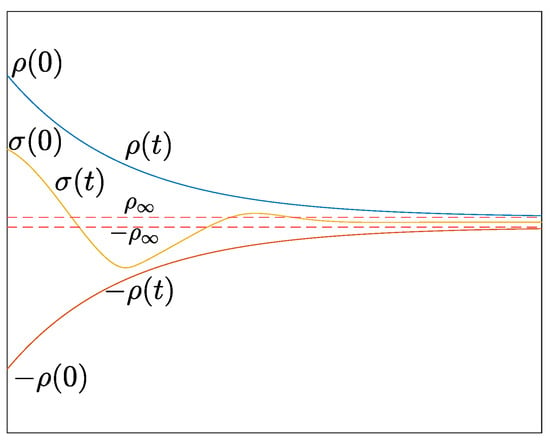
Figure 1.
Graphical representation of (16).
The function is a smooth, bounded, strictly positive and decreasing function of time called performance function and is chosen as follows:
with and l being positive gains that are chosen to satisfy the designer’s specifications. Specifically,
- is selected according to the maximum allowable tracking error at the steady state;
- l determines a lower bound on the speed of convergence;
- affects the maximum overshoot and is selected such that .
For the scalar error , we define the linear filtered error:
where is a positive constant and denotes the tracking error. In addition, consider the normalized error and the transformation that maps the constrained behavior as defined in (16), into an unconstrained one. More specifically, is a strictly increasing, symmetric and bijective mapping, e.g., . Finally, prescribed performance is achieved by employing the following control law []:
where k is a positive gain.
4.4. Iterative Learning
The identification algorithm involves an iterative process, aiming to enhance the approximation of the unknown underlying dynamics until convergence is reached (i.e., , where is an arbitrarily small positive value). More specifically, we adopt an artificial neural network with any number of hidden layers and sigmoidal activation functions, which is trained based on the collected data over a series of reference trajectories. The aforementioned training process takes place in a supervised learning environment, where the necessary input–output data for the estimation of the network’s weights at each iteration are acquired by tracing a reference trajectory designed through the process outlined in Section 4.2.
However, in order to guarantee that the final result is devoid of bias along a specific trajectory, a distinct random sequence of points is employed to construct the reference trajectory in each iteration. In addition, to ensure accurate tracking, the aforementioned trajectory will be tracked with predefined transient and steady-state performance using the PPC technique, as described in Section 4.3. During each instance of learning, the weights of the neural network are obtained by optimizing the matching between the network’s output and the target values via a backpropagation algorithm. Notice that under Assumption 2, the system’s state (i.e., the input training data) is available for measurement. However, since we do not have access to , the target output values to train the neural network are not available.
To overcome this challenge, during each iteration the following tracking differentiator [] is employed:
with positive gains . When , then based on [], and consequently , from which we may derive the input–output pair that will be employed for the training process. Notice that during the first round () over the closed reference trajectory, the structure in (20) is not initialized yet, as we have not gathered the necessary data. Therefore, the network is activated after the first training stage has taken place. As a result, in each subsequent round (m), the extracted neural structure originates from the previous iteration. After each round of training, the obtained knowledge regarding the system’s dynamics is employed not only to enhance the estimation of but also to provide improved initial weights for the consecutive iterations. Consequently, an accurate model of the system dynamics can be acquired after sufficient iterations (e.g., when the weights do not change above a threshold). The complete algorithm for the iterative learning of the unknown dynamics is summarized in Algorithm 2.
Remark 1.
The collection of transition points and their corresponding times that are utilized in the design of the online reference trajectories, as described in Algorithm 1, is an offline procedure. Consequently, once the trajectories have been generated, the problem is reduced to a tracking control problem with the PPC scheme, which is efficiently tackled owing to the low complexity control signal. In a similar manner, once the tracking of the reference trajectories is complete, we have successfully acquired all the necessary data that will be employed in the final part of Algorithm 2, in order to train the adopted neural structure. Therefore, we stress that our approach can be employed to tackle identification of complex systems without sacrificing online performance since the computational burden mainly stems from offline procedures.
| Algorithm 2 Iterative Learning |
|
5. Results
In this section, we demonstrate the effectiveness of the proposed identification scheme with the goal of obtaining the underlying system dynamics of a two-degree of freedom robotic manipulator without assuming any prior knowledge, via two scenarios: a simulated one, showcasing the full capabilities of our method, and a real-life experiment to demonstrate the applicability of our algorithm to real-world systems.
5.1. Simulation Study
Initially, we present the simulation results for the successful identification of the unknown dynamics of a two-degree of freedom robotic manipulator, as illustrated in Figure 2. All simulations were conducted in MATLAB R2023a. The robotic manipulator obeys the following dynamic model
where and denote the joint angular positions and velocities, respectively, is a positive definite inertia matrix, is the matrix that describes the Coriolis–centrifugal phenomena, is the vector describing the influence of gravity and is the torque that acts as the system’s input. More specifically, the inertia matrix is formulated as
where
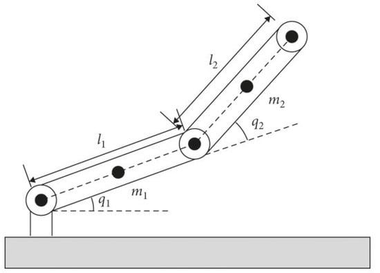
Figure 2.
Two-DOF robotic manipulator.
In addition, the vector containing the Coriolis and centrifugal torques is defined as follows:
with c being . Additionally, the gravity vector is given by:
and the terms and correspond to and , respectively. The values adopted for simulation are provided in Table 1, with , and denoting the mass, the moment of inertia and the length of link i, respectively, being the joint friction coefficient and g the acceleration of gravity. The aforementioned dynamics can be expressed as , aligning with the form described in Section 3. Our goal is to learn the unknown nonlinear mapping f over the domain set for .

Table 1.
System parameter values.
To achieve this, a reference trajectory traversing in random order 27 points scattered over the domain set is designed. A closed path of 27 such points, along with the workspace are depicted in Figure 3. It is evident that the generated trajectory, which traverses all points, spans a significant part of the desired state space. In order to obtain the time of transition between the points of the sequence, the performance index (13) was minimized, with the weighting parameters set as , and . Subsequently, a PPC controller with gains , and specifications , , , , and is used to track the reference trajectory. Finally, the gains of the tracking differentiator are set to and . In Figure 4 and Figure 5, the tracking of one of the reference signals by the PPC controller is depicted, along with the error and the control input, for both of the manipulator’s joints.
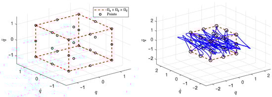
Figure 3.
The workspace (left) and a closed path (blue) traversing it (right).
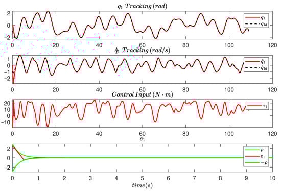
Figure 4.
The tracking responses of and , the evolution of the tracking error and the control input under PPC.
Figure 5.
The tracking responses of and , the evolution of the tracking error and the control input under PPC.
In addition, for the training process, a single hidden-layer neural network with 15 neurons was utilized. To elaborate further on this, 15 different reference trajectories were formed by permuting the 27 points of the workspace to sufficiently improve iteratively the estimation of the underlying dynamics. During each iteration, data are collected by tracking a different reference trajectory with the PPC controller. The gathered data are fed to the neural network, whose training is conducted by the MATLAB toolbox employing the default Levenberg–Marquardt algorithm. After the first iteration, the resulting network is employed in the tracking differentiator to improve both the acceleration estimation and the selection of the initial weights for the consecutive iterations. To avoid overfitting of the employed neural network and achieve satisfactory generalization capabilities, after tracking the reference trajectories, the acquired dataset was split into a training and a testing set, with a ratio of 85% and 15%, respectively. This was to ensure that the acquired neural structure performs well, not only on the training set, but also on the unseen data represented by the testing set.
In Figure 6, the curve fitting evolution for both components of the unknown dynamics can be observed. Furthermore, by comparing the initial estimations in Figure 7 with the results of the approximation problem in Figure 8, it becomes evident that the proposed scheme has resulted in a highly accurate estimate of the system dynamics with no dependence on any prior knowledge. We stress that to ensure that the evaluation of the identification scheme is free of bias, the testing is conducted using a reference trajectory different from the ones employed during the training stages.
Figure 6.
Improvement of fitting during iterations for a testing dataset.
Figure 7.
Actual values and estimates of after the first iteration.
Figure 8.
Actual values and estimates of at the end of the iterative process.
5.2. Experimental Study
This section showcases the results of an experimental study which validates the effectiveness and applicability of the proposed scheme in a real-world system. Towards this direction, we consider the two-degree of freedom planar robot manipulator with DC geared motor actuation, depicted in Figure 9. Measurements regarding the system’s state (i.e., position and velocity) for each joint are obtained through a rotary encoder attached at each motor’s shaft. Furthermore, a microcontroller was employed to acquire the necessary sensor data as well as to drive the motors. This is achieved through utilization of a motor driver that allows the direction and speed of a DC motor to be adjusted by using a Pulse–Width-Modulated (PWM) signal.
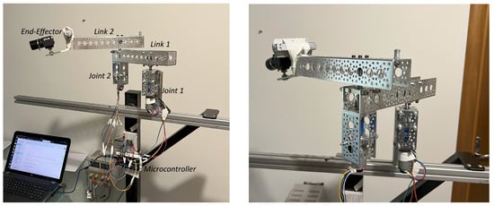
Figure 9.
Two-DOF robotic manipulator.
In order to calculate the applied input control signal, note that the produced torque is given by:
where denotes the armature current and is the motor torque constant. Moreover, at a constant operating point, by applying Kirchoff’s Voltage Law, we obtain:
where is the supplied voltage, denotes the armature’s resistance, while denotes the angular velocity and and are the back-EMF voltage and constant, respectively. By applying the law of conservation of energy, it can be shown that = , and therefore, the applied control input signal can be approximately obtained as follows:
Finally, the constant can be obtained by dividing the rated voltage of each motor by its no-load speed. For the motors employed in our experiment, the following parameter values were extracted: , , and .
Similarly to the previous study, we aim at learning the unknown nonlinear mapping f over the domain set for ; therefore, a reference trajectory traversing in random order 27 points scattered over the domain set is designed. The time of transition between the points of the sequence was obtained by minimizing the performance index (13), with the weighting parameters set as , and . Subsequently, a PPC controller with gains and and specifications , , , , , is used to track the reference trajectory. In Figure 10 and Figure 11, the tracking of one of the reference signals by the PPC controller is depicted, along with the control input, for both of the robot’s joints. A Savitzky–Golay filter [] was used to eliminate the noise of the experimental data. In addition, a video of the robotic manipulator tracking a reference trajectory of 27 points using the PPC technique can be accessed through the following hyperlink: https://youtu.be/CrUUgfKE6t4 (accessed on 27 February 2024).
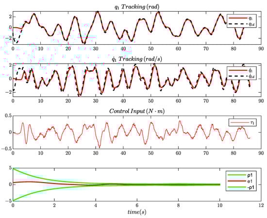
Figure 10.
The tracking responses of and , the evolution of the tracking error and the control input under PPC.
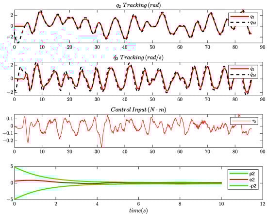
Figure 11.
The tracking responses of and , the evolution of the tracking error and the control input under PPC.
In the initial phase of the experiment, we track 20 different reference trajectories and store the obtained data (i.e., position, velocity and applied torque) that will be used in the next phase to iteratively improve the underlying dynamics estimation. In the learning phase, the gathered data along with the target acceleration output (which is obtained through a tracking differentiator as described in Section 4.4) are fed to a single hidden-layer neural network with 15 neurons whose training is conducted by the MATLAB toolbox employing the default Levenberg–Marquardt algorithm. Similar to the simulation study, overfitting of the employed neural network is avoided by splitting the acquired dataset into a training and a testing set, with a ratio of 85% and 15%, respectively. After the first iteration, the resulting network is utilized in the tracking differentiator, whose gains are set to , and , to improve both the acceleration estimation and the selection of the initial weights for the consecutive iterations. To evaluate the learning capabilities of the identification scheme, a reference trajectory different from the ones employed during the training stages was used to compare the results of the approximation problem. More specifically, the initial and final estimations of the unknown dynamics are provided in Figure 12 and Figure 13, where decreases in the Root Mean Square Error (RMSE) of and are witnessed for the underlying dynamics and , respectively. It is clear that the suggested approach yields an adequate estimation of the system dynamics, without relying on any prior knowledge.
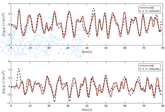
Figure 12.
Actual values and estimates of after the first iteration.
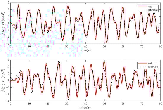
Figure 13.
Actual values and estimates of at the end of the iterative process.
6. Conclusions and Future Work
In this work, we present an iterative learning process that aims at extracting the unknown nonlinear dynamics of a plant in the targeted system state space. The approach was demonstrated through both an extensive simulation study and a real-life experiment on a robotic manipulator with two degrees of freedom. Our main contributions consist of a novel reference trajectory generation scheme that is capable of sufficiently exciting the underlying dynamics and an iterative algorithm that progressively improves the unknown parameters of the employed neural network, even in the case of open-loop instability. Future formal approaches should consider tackling the issue of input and state constraints through the design of a trajectory that inherently avoids configurations associated with physical system constraints/limitations (e.g., mechanical constraints).
Author Contributions
Conceptualization, C.P.B.; methodology, C.P.B.; software, C.V. and F.T.; validation, C.V. and F.T.; formal analysis, C.V. and F.T.; investigation, all; resources, C.P.B.; data curation, C.V. and F.T.; writing—original draft preparation, C.V.; writing—review and editing, C.P.B. and G.C.K.; visualization, C.V. and F.T.; supervision, C.P.B.; project administration, C.P.B. and G.C.K.; funding acquisition, C.P.B. and G.C.K. All authors have read and agreed to the published version of the manuscript.
Funding
The work of C.V. and C.P.B. was funded by the Hellenic Foundation for Research and Innovation (H.F.R.I.) under the second call for research projects to support postdoctoral researchers (HFRI-PD19-370).
Data Availability Statement
Data for this study are available from the corresponding author on request.
Conflicts of Interest
The authors declare no conflicts of interest.
References
- Volterra, V. Sopra le Funzioni Che Dipendono da Altre Funzioni; Tipografia della R. Accademia dei Lincei: Rome, Italy, 1887. [Google Scholar]
- Birpoutsoukis, G.; Marconato, A.; Lataire, J.; Schoukens, J. Regularized nonparametric Volterra kernel estimation. Automatica 2017, 82, 324–327. [Google Scholar] [CrossRef]
- Dalla Libera, A.; Carli, R.; Pillonetto, G. Kernel-based methods for Volterra series identification. Automatica 2021, 129, 109686. [Google Scholar] [CrossRef]
- Xu, Y.; Mu, B.; Chen, T. On Kernel Design for Regularized Volterra Series Model with Application to Wiener System Identification. In Proceedings of the 2022 41st Chinese Control Conference (CCC), Hefei, China, 25–27 July 2022; pp. 1503–1508. [Google Scholar] [CrossRef]
- Nelles, O. Nonlinear Dynamic System Identification. In Nonlinear System Identification: From Classical Approaches to Neural Networks and Fuzzy Models; Springer: Berlin/Heidelberg, Germany, 2001; pp. 547–577. [Google Scholar] [CrossRef]
- Wills, A.; Schön, T.B.; Ljung, L.; Ninness, B. Identification of Hammerstein–Wiener models. Automatica 2013, 49, 70–81. [Google Scholar] [CrossRef]
- Li, L.; Zhang, J.; Wang, F.; Zhang, H.; Ren, X. Binary-Valued Identification of Nonlinear Wiener–Hammerstein Systems Using Adaptive Scheme. IEEE Trans. Instrum. Meas. 2023, 72, 3001110. [Google Scholar] [CrossRef]
- Chen, S.; Billings, S.A. Representations of non-linear systems: The NARMAX model. Int. J. Control 1989, 49, 1013–1032. [Google Scholar] [CrossRef]
- Abdul Rahim, N.; Taib, M.N.; Adom, A.; Abdul Halim, M.A. Nonlinear System Identification for a DC Motor using NARMAX Model with Regularization Approach. In Proceedings of the International Conference on Control, Instrumentation and Mechatronics Engineering (CIM’07), Johor, Malaysia, 28–29 May 2007. [Google Scholar]
- Al-Mahturi, A.; Santoso, F.; Garratt, M.A.; Anavatti, S.G. Online System Identification for Nonlinear Uncertain Dynamical Systems Using Recursive Interval Type-2 TS Fuzzy C-means Clustering. In Proceedings of the 2020 IEEE Symposium Series on Computational Intelligence (SSCI), Canberra, Australia, 1–4 December 2020; pp. 1695–1701. [Google Scholar] [CrossRef]
- Zou, W.; Zhang, N. A T-S Fuzzy Model Identification Approach Based on a Modified Inter Type-2 FRCM Algorithm. IEEE Trans. Fuzzy Syst. 2018, 26, 1104–1113. [Google Scholar] [CrossRef]
- Ferdaus, M.M.; Pratama, M.; Anavatti, S.; Garratt, M. Online Identification of a Rotary Wing Unmanned Aerial Vehicle from Data Streams. Appl. Soft Comput. 2018, 76, 313–325. [Google Scholar] [CrossRef]
- Hornik, K.; Stinchcombe, M.; White, H. Multilayer feedforward networks are universal approximators. Neural Netw. 1989, 2, 359–366. [Google Scholar] [CrossRef]
- Delgado, A.; Kambhampati, C.; Warwick, K. Dynamic recurrent neural network for system identification and control. Control Theory Appl. IEE Proc. 1995, 142, 307–314. [Google Scholar] [CrossRef]
- Al Seyab, R.; Cao, Y. Nonlinear system identification for predictive control using continuous time recurrent neural networks and automatic differentiation. J. Process. Control 2008, 18, 568–581. [Google Scholar] [CrossRef]
- Sen, G.D.; Gunel, G.Ö.; Guzelkaya, M. Extended Kalman Filter Based Modified Elman-Jordan Neural Network for Control and Identification of Nonlinear Systems. In Proceedings of the 2020 Innovations in Intelligent Systems and Applications Conference (ASYU), Istanbul, Turkey, 15–17 October 2020; pp. 1–6. [Google Scholar] [CrossRef]
- Ni, J.; Ahn, C.K.; Liu, L.; Liu, C. Prescribed performance fixed-time recurrent neural network control for uncertain nonlinear systems. Neurocomputing 2019, 363, 351–365. [Google Scholar] [CrossRef]
- Kang, H.H.; Su Lee, S.; Kim, K.S.; Ki Ahn, C. Finite Memory Estimation-Based Recurrent Neural Network Learning Algorithm for Accurate Identification of Unknown Nonlinear Systems. In Proceedings of the 2019 IEEE Symposium Series on Computational Intelligence (SSCI), Xiamen, China, 6–9 December 2019; pp. 470–475. [Google Scholar] [CrossRef]
- Kang, H.H.; Ahn, C.K. Neural Network-Based Moving Window Iterative Nonlinear System Identification. IEEE Signal Process. Lett. 2023, 30, 1007–1011. [Google Scholar] [CrossRef]
- Kumar, R. Memory Recurrent Elman Neural Network-Based Identification of Time-Delayed Nonlinear Dynamical System. IEEE Trans. Syst. Man Cybern. Syst. 2023, 53, 753–762. [Google Scholar] [CrossRef]
- Chen, M.; Ge, S.S.; How, B.V.E. Robust Adaptive Neural Network Control for a Class of Uncertain MIMO Nonlinear Systems With Input Nonlinearities. IEEE Trans. Neural Netw. 2010, 21, 796–812. [Google Scholar] [CrossRef]
- He, W.; Chen, Y.; Yin, Z. Adaptive Neural Network Control of an Uncertain Robot With Full-State Constraints. IEEE Trans. Cybern. 2016, 46, 620–629. [Google Scholar] [CrossRef]
- Wang, M.; Wang, C. Neural learning control of pure-feedback nonlinear systems. Nonlinear Dyn. 2014, 79, 2589–2608. [Google Scholar] [CrossRef]
- Liu, T.; Wang, C.; Hill, D.J. Learning from neural control of nonlinear systems in normal form. Syst. Control Lett. 2009, 58, 633–638. [Google Scholar] [CrossRef]
- Wang, C.; Wang, M.; Liu, T.; Hill, D.J. Learning From ISS-Modular Adaptive NN Control of Nonlinear Strict-Feedback Systems. IEEE Trans. Neural Netw. Learn. Syst. 2012, 23, 1539–1550. [Google Scholar] [CrossRef]
- Dai, S.L.; Wang, C.; Wang, M. Dynamic Learning From Adaptive Neural Network Control of a Class of Nonaffine Nonlinear Systems. IEEE Trans. Neural Netw. Learn. Syst. 2014, 25, 111–123. [Google Scholar] [CrossRef]
- Wang, M.; Wang, C. Learning From Adaptive Neural Dynamic Surface Control of Strict-Feedback Systems. IEEE Trans. Neural Netw. Learn. Syst. 2015, 26, 1247–1259. [Google Scholar] [CrossRef]
- Wang, M.; Wang, C.; Liu, X. Learning from adaptive neural control with predefined performance for a class of nonlinear systems. In Proceedings of the 33rd Chinese Control Conference, Nanjing, China, 28–30 July 2014; pp. 8871–8876. [Google Scholar] [CrossRef]
- Wang, C.; Hill, D. Learning from neural control. IEEE Trans. Neural Netw. 2006, 17, 130–146. [Google Scholar] [CrossRef]
- Zisis, K.; Bechlioulis, C.P.; Rovithakis, G.A. Control-Enabling Adaptive Nonlinear System Identification. IEEE Trans. Autom. Control 2022, 67, 3715–3721. [Google Scholar] [CrossRef]
- Byrnes, C.; Isidori, A. Asymptotic stabilization of minimum phase nonlinear systems. IEEE Trans. Autom. Control 1991, 36, 1122–1137. [Google Scholar] [CrossRef]
- Kurdila, A.; Narcowich, F.; Ward, J. Persistency of Excitation in Identification Using Radial Basis Function Approximants. Siam J. Control Optim. 1995, 33, 625–642. [Google Scholar] [CrossRef]
- Bechlioulis, C.P.; Rovithakis, G.A. Robust Adaptive Control of Feedback Linearizable MIMO Nonlinear Systems With Prescribed Performance. IEEE Trans. Autom. Control 2008, 53, 2090–2099. [Google Scholar] [CrossRef]
- Dimanidis, I.S.; Bechlioulis, C.P.; Rovithakis, G.A. Output Feedback Approximation-Free Prescribed Performance Tracking Control for Uncertain MIMO Nonlinear Systems. IEEE Trans. Autom. Control 2020, 65, 5058–5069. [Google Scholar] [CrossRef]
- Lewis, F.L.; Vrabie, D.; Syrmos, V.L. Optimal Control Of Continuous-Time Systems. In Optimal Control; John Wiley & Sons, Ltd.: Hoboken, NJ, USA, 2012. [Google Scholar] [CrossRef]
- Brent, R.P. Algorithms for Minimization without Derivatives; Prentice-Hall: Englewood Cliffs, NJ, USA, 1973; p. 195. [Google Scholar]
- Guo, B.Z.; Zhao, Z. On convergence of tracking differentiator. Int. J. Control 2011, 84, 693–701. [Google Scholar] [CrossRef]
- Savitzky, A.; Golay, M.J.E. Smoothing and differentiation of data by simplified least squares procedures. Anal. Chem. 1964, 36, 1627–1639. [Google Scholar] [CrossRef]
Disclaimer/Publisher’s Note: The statements, opinions and data contained in all publications are solely those of the individual author(s) and contributor(s) and not of MDPI and/or the editor(s). MDPI and/or the editor(s) disclaim responsibility for any injury to people or property resulting from any ideas, methods, instructions or products referred to in the content. |
© 2024 by the authors. Licensee MDPI, Basel, Switzerland. This article is an open access article distributed under the terms and conditions of the Creative Commons Attribution (CC BY) license (https://creativecommons.org/licenses/by/4.0/).