Quantifying the Inverter-Interfaced Renewable Energy Critical Integration Capacity of a Power Grid Based on Short-Circuit Current Over-Limits Probability

Abstract

Power systems with a high proportion of inverter-based sources like photovoltaics require a substantial short-circuit current ratio to ensure strong voltage support capabilities. However, this also increases the system’s short-circuit current capacity and levels, which may potentially affect the safe operation of system equipment and current-carrying conductors. To evaluate the operational risks, this paper proposes a quantitative calculation model for the critical integration proportion of grid-connected inverter-interfaced power sources based on short-circuit current over-limit probability. Firstly, according to the verification criterion about short-circuit current during the selection of the switching equipment and conductors in the power system, the short-circuit current over-limit probability evaluation system with five indices is established. Secondly, considering the impact of the increased grid integration proportion of inverter-based power sources on short-circuit currents, an evaluation process for operational risk probabilities is proposed. Based on this, the critical access proportion for inverter-based power source integration in the power grid can be calculated. Finally, the proposed model is used to assess the operational risk probability for a 220 kV system which includes a high proportion of inverter-based power sources in the Anhui area, China. Through the analysis of cumulative probability distribution curves, the critical grid integration proportion interval for the transition from normal to high proportion stages of inverter-based power sources is determined.

1. Introduction

In recent years, facing the challenge of depleting fossil fuel resources and escalating environmental concerns, renewable energy sources (RES) such as wind power (WP) and photovoltaics (PV) have experienced rapid growth [1,2]. To achieve the global climate targets and carbon neutrality goals set for 2050, the penetration level of RESs within the power grid is continuously increasing [3]. However, the grid integration of PV and PV generation through inverter-based power sources introduces a challenge. The power electronic interfaces of these power sources can elevate the level of short-circuit currents in the system, potentially compromising the reliability of the power system and the safety of operation equipment [4]. Moreover, the characteristics of grid integration vary significantly at different levels of integration proportion [5,6]. Therefore, it is crucial to analyze the critical threshold at which the increased proportion of inverter-based power source integration begins to impact the safe operational risk of the system.

In 1975, B. Sørensen first proposed the idea of developing a power system entirely powered by RESs [7]. Since then, the proportion of inverter-based power sources including WP and PV within the power system has emerged as a key metric for assessing the system’s development. Currently, the integration proportion of inverter-based power sources is defined in two primary ways: (i) the ratio of the installed capacity of inverter-based power sources to the peak load of the power system; and (ii) the proportion of electricity generated from inverter-based power sources relative to total electricity use [8,9]. Among them, the former, focusing on installed capacity versus peak load, is more commonly adopted and is the approach utilized in our study.

In the study of high proportion characteristics of grid-connected inverter-based power sources, the research in [10] suggests that an increase in the grid integration proportion of inverter-based sources heightens the uncertainty of the power system, affecting the system’s flexibility balance. Reference [11] reveals that a high proportion of inverter-based power source integration introduces complexity into the grid infrastructure, resulting in intricate and fluctuating power flow patterns. Reference [12] emphasizes that a high integration level of inverter-based power sources significantly elevates the risk of voltage-related issues in distribution networks, encompassing voltage exceedances, voltage imbalances, and fluctuations in power. Reference [13] points out that an increased proportion of inverter-based power source integration could cause line power flows to reach thermal stability limits. Research in [14] demonstrates that the conventional distance relay on grid-connected inverter-based power sources has a high risk of malfunctioning or refusing to operate.

As the grid integration of inverter-based power sources continues to evolve, the power electronics equipment on the source side is driving a transition from traditional electromechanical grid equipment to power electronics-based systems [15]. Several studies have used the electrification of power systems to gauge the developmental stages of inverter-based power source integration. Reference [16] suggests that an increase in the proportion of inverter-based power source integration adds more power electronic interfaces to the power system, thereby reducing system inertia and altering the mechanisms of stability. References [17,18] note that due to the limited voltage endurance and current-carrying capacity of power electronic devices, an increase in the proportion of inverter-based power sources can lead to ambiguous fault current characteristics and limited magnitudes.

However, the references above cannot provide a quantitative assessment of the impacts on power systems after high proportion integration of inverter-based power sources. Besides, they fail to offer a clear boundary for the transition from normal to high proportion stages in the development of inverter-based power source integration in the power system. Consequently, specific principles for defining “high proportion” stages for a power system are not presented.

To address these issues, this paper introduces an operational risk evaluation framework based on short-circuit current over-limit probability to calculate the critical integration proportion of inverter-based power sources. First, by proposing five indices based on short-circuit current over-limit, an operational risk assessment system for the power grid is constructed. Then, considering the impact of increasing inverter-based power source integration proportions on short-circuit currents, an evaluation process for assessing the probability of operational risks is proposed to calculate the critical integration proportion of inverter-based power sources under the high-ratio stage. Finally, through a case study based on an actual power grid, the proposed model demonstrates its capability to accurately determine the critical integration proportion of inverter-based power sources under the high-ratio stage using various indices.

The remainder of this paper is organized as follows: Section 2 introduces five representative indices to quantify short-circuit current over-limit risk under high inverter-based power sources integration. Then, Section 3 presents the probabilistic operational risk assessment process for short-circuit current over-limit and the calculation method for critical integration proportion of inverter-based power sources under the high ratio stage. In Section 4, the numerical analysis is conducted to verify the proposed approach. Finally, the study is summarized and concluded in Section 5.

2. Indices of Short-Circuit Current Over-Limits Probability for High Proportion Grid-Connected Inverter-Based Power Sources Integration

In this paper, focusing on the operational safety of switching devices and conductors within the power system, a group of risk indices is established to quantify operational risks that arise from the increased short-circuit currents due to the escalating integration of inverter-based power sources into the power system.

2.1. Short-Circuit Current Breaking Failure Probability (SCCBFP)

The key to the normal opening and closing of a switch lies in the extinguishing of the electric arc. The main factor sustaining the arc’s combustion is thermal ionization, which depends on the root mean square (RMS) value of the current [19]. Therefore, the short-circuit current breaking failure probability (SCCBFP) index is proposed to measure the probability that the short-circuit current exceeds the breaking current capacity of the switch. In this paper, the assessment of this index utilizes the RMS value of the power system’s short-circuit current during a three-phase short circuit. It is widely accepted that a failure to interrupt occurs when the RMS value of the system’s short-circuit current surpasses the maximum interrupting capacity of the switch I_dl (which can be found by looking up tables). The evaluation method is shown in Equation (1):

$$SCCBFP=P(I_m>I_{dl})=\frac{M_{SCCBFP}}{M},$$

(1)

where I_m represents the maximum RMS value of the system short-circuit current during a three-phase short circuit; M_SCCBFP denotes the frequency with which I_m exceeds I_dl; and M is the total number of fault samples taken.

2.2. Equipment Dynamic Stability Failure Probability (EDSFP)

The equipment dynamic stability failure probability (EDSFP) is formulated to represent the probability of exceeding the maximum electrodynamic impact that the mechanical structure can withstand when the switch cuts off the short-circuit current [19]. The electromechanical force borne by the mechanical parts of the switch depends on the instantaneous value of the current; thus, the maximum current at the time of fault should be considered [20]. Accordingly, this paper selects the system short-circuit impact current occurring during a three-phase short circuit to assess this index. It is widely accepted that an electromechanical stability failure occurs when the impact current exceeds the dynamic stability current I_dw of the switch (which can be found by looking up tables). The evaluation method is presented as Equation (2):

$$EDSFP=P(I_{ch}>I_{dw})=\frac{M_{EDSEP}}{M},$$

(2)

where I_ch is the system short-circuit impact current during a three-phase short circuit. M_EDSEP represents the frequency with which I_ch exceeds I_dw.

2.3. Equipment Thermal Stability Failure Probability (ETSFP)

The equipment thermal stability failure probability (ETSFP) index refers to the probability of exceeding the short-term thermal endurance of its metal and insulation materials for the switch when conducting a short-circuit current [21]. When the switch has already been operating at its rated state and has reached the maximum permissible temperature θ_N·xu, a sudden increase in current to a certain value I_t for t_I seconds (both I_t and t_I can be obtained by looking up tables) can lead to a temperature rise to the maximum short-term thermal limit θ_f·xu as specified by design standards. In this situation, the integrity of the switch should still be maintained [19]. Therefore, this paper assesses this index by using the RMS value of the system short-circuit current occurring during a three-phase short circuit. The evaluation method is presented as Equation (3):

$$ETSEP=P({\displaystyle \underset{0}{\overset{t}{\int }}{i}_d^2}dt>I_t^2{t}_I)=\frac{M_{ETSEP}}{M},$$

(3)

where the i_d represents the RMS value of the system short-circuit current during a three-phase fault. M_EDSEP indicates the frequency with which the heat generated by the short-circuit current during the fault duration exceeds the maximum short-term thermal limit allowed for the switch.

The blue curve in Figure 1 illustrates the general curve of the system short-circuit current RMS value over fault duration which is widely adopted in short-circuit current calculations [22,23]. Although the actual curve may vary with changes in system parameters, the curve in Figure 1 summarizes the general characteristics of short-circuit currents over different phases in a time series. At moment t₀, a three-phase short circuit occurs. At moment t₁, the RMS value of the short-circuit current reaches its maximum. At moment t₂, the system enters a steady state, with I_∞ representing the steady-state short-circuit current RMS value. By applying the trapezoidal rule for integration [24], the entire area under the fault current versus time curve can be divided into three parts, denoted as S₁–S₃, as shown in the figure, therefore

$${\displaystyle \underset{0}{\overset{t}{\int }}{i}_d^2}dt=\frac{1}{2}(t_1-t_0)I_m+\frac{1}{2}(I_m+I_{\infty })(t_2-t_1)+(t_I-t_2)I_{\infty }.$$

(4)

Therefore, the ETSFP can be calculated by

$$\begin{array}{ll}ETSEP=& P(\frac{1}{2}(t_1-t_0)I_m+\frac{1}{2}(I_m+I_{\infty })(t_2-t_1)\\ & +(t_I-t_2)I_{\infty }>I_t^{2}t)=\frac{M_{ETSEP}}{M},\end{array}$$

(5)

where M_ETSEP represents the frequency at which the heat generated during an actual short-circuit period exceeds the switch’s allowable short-time heating value.

2.4. Conductor Short-Term Heating Temperature Over-Limit Probability (CSHTOP)

The fundamental condition for the thermal stability of a conductor under short-circuit current is that the maximum temperature due to short-time heating does not exceed the allowable limit θ_xu [19] (which can be obtained by looking up tables). Consequently, the evaluation method for the probability of the conductor short-term heating temperature over-limit probability (CSHTOP) is

$$CSHTOP=P({\theta }_k>{\theta }_{xu})=\frac{M_{CSHTOP}}{M},$$

(6)

where θ_k represents the temperature of the conductor during an actual short-circuit heating event. M_CSHTOP denotes the frequency at which the temperature of the conductor after short-time heating exceeds the maximum allowable temperature for short-time heating.

In the calculation of short-time heating of conductors, it is assumed that the heat dissipation power is neglected, and all the heat provided by the short-circuit current is consumed in raising the temperature of the conductor [25]. Therefore, the heat supplied by the short-circuit current Q_d is calculated by

$$Q_d={\displaystyle {\int }_0^{t_d}{i}_d^2\mathrm{d}t},$$

(7)

where i_d represents the RMS value of the short-circuit current RMS value flowing through the conductor. t_d is the actual duration of the short-circuit.

The heat content per unit volume of the conductor after short-time heating A_k is calculated as follows:

$$A_k=A_0+\frac{1}{S^2}{Q}_d,$$

(8)

where A₀ is the heat content per unit volume of the conductor at the start of the short-circuit. S is the cross-sectional area of the conductor, in mm². The temperature of the conductor after short-time heating θ_k can be obtained by consulting the curve that relates the material’s heat content to temperature after A_k is calculated.

In engineering applications, the minimum cross-sectional area is commonly used to ensure the thermal stability of a conductor. Specifically, the requirement is

$$S_f=\frac{I_{\infty }}{C}\sqrt{K_j{t}_j},$$

(9)

where C represents the material’s heat resistance value, which is related to the conductor material and heating temperature, which can be found in electrical design manuals. K_j is the skin effect coefficient for the conductor, and it can be ignored when K_j < 1. S_f is the equivalent cross-sectional area of the conductor during short-time heating measured in mm². To align with engineering applications, the evaluation method for the probability CSHTOP is modified as

$$CSHTOP=P(S_f>S)=\frac{M_{CSHTOP}}{M},$$

(10)

where M_CSHTOP denotes the frequency at which the equivalent cross-sectional area during short-time heating exceeds the actual cross-sectional area of the conductor.

2.5. Rigid Conductor Instantaneous Maximum Stress Over-Limit Probability (RCIMSOP)

Rigid conductors require verification of dynamic stability during a short circuit [26], while flexible conductors do not require verification. The fundamental condition for ensuring conductor dynamic stability is that the maximum stress generated in the conductor’s cross-section σ_max (N/cm²) does not exceed the material’s allowable stress σ₀ (which can be determined by looking up tables). The evaluation method for the rigid conductor instantaneous maximum stress over-limit probability (RCIMSOP) is as follows:

$$RCIMSOP=P({\sigma }_{\max }>{\sigma }_{xu})=\frac{M_{RCIMSOP}}{M},$$

(11)

where M_RCIMSOP denotes the frequency at which the maximum stress σ_max generated after a short circuit exceeds the allowable stress σ_xu. The maximum electromotive force on the conductor following a fault is generated by the impact current, and the maximum electromotive force and the bending moment it creates within a span are as follows:

$$F_{\max }=1.73I_{ch}^2\frac{l}{a}\times {10}^{-1},$$

(12)

$$M_F=\frac{F_{\max }l}{10}=1.73I_{ch}^2\frac{l^2}{a}\times {10}^{-2},$$

(13)

where F_max is the maximum electromotive force generated by the system’s short-circuit impact current within a span measured in “N” with the impact current measured in “kA”. M_F is the bending moment formed by the maximum electromotive force, l is the busbar span (i.e., the distance between two supports, cm). a is the phase-to-phase distance (i.e., the moment of the conductor center, m). Rigid conductors require an internal and external stress balance to maintain dynamic stability, where the maximum external bending moment is σW. σ represents the stress in the conductor material (N/cm²). W represents the conductor’s section modulus against bending (cm³), which is related to the cross-sectional size and arrangement of the conductors. Therefore,

$$\sigma W=M.$$

(14)

Given that the span of rigid conductors is clearly defined in engineering construction, the span can conveniently be used as an evaluation metric for the probability of exceeding the instantaneous maximum stress limit of rigid conductors for engineering applications. Once system parameters are established, the material properties of the conductors σ_xu and W are consequently determined. This allows for the calculation of the maximum stress required to maintain dynamic stability under short-circuit conditions, as follows:

$${\sigma }_{\max }=F_{\max }l/10W.$$

(15)

3. Probabilistic Operational Risks Assessment and Critical Access Proportion Calculation for High Proportion Grid-Connected Inverter-Based Power Sources Integration

In this section, the regulation for increasing the installed capacity of inverter-based power sources in the power grid is formulated first. Then, the overall process for evaluating the short-circuit current over-limit probability is outlined for assessing the operational risk probability. Finally, the method for calculating the critical integration proportion for high-ratio inverter-based power sources. Finally, the principles for categorizing different stages for the grid integration of inverter-based power sources are proposed with the help of operational risk evaluation.

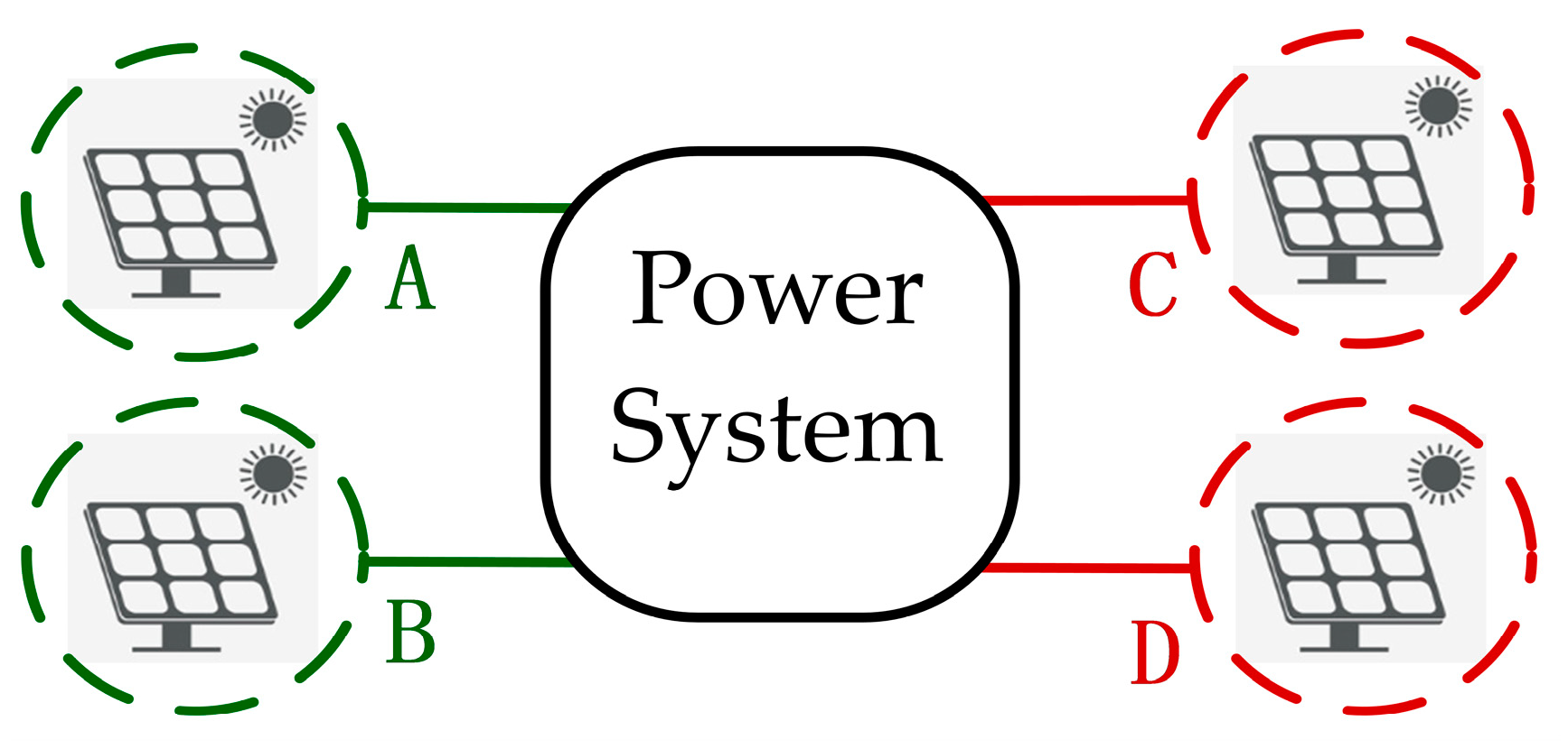
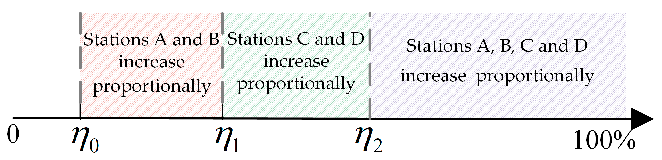
3.1. Regulations for Enhancing the Proportion of Inverter-Based Power in Grid Integration

The proportion of grid-connected inverter-based power sources refers to the ratio between the installed capacity of inverter-based power sources and the system’s maximum load. There are two methods for increasing the installed capacity of inverter-based sources: directly expanding the capacity at existing sites or constructing new inverter-based power stations. Different expansion approaches have varying impacts on the system’s short-circuit current. To facilitate analysis, this paper defines the following regulations for increasing the installed capacity of inverter-based power sources.

As shown in Figure 2, stations A and B represent existing inverter-based power stations, while stations C and D are newly selected sites. The current proportion of inverter-based power sources integrated into the grid is η₀. According to the regulation of this paper, during capacity expansion, stations A and B first increase their capacity proportionally until reaching a share of η₁. Subsequently, new stations C and D are constructed at the newly selected sites, with their installed capacity increasing proportionally until achieving a share of η₂. Finally, according to planning requirements, stations A, B, C, and D are jointly increased in proportion until the combined share reaches 100%, as illustrated in Figure 3.

The above process can be formulated as follows:

$${\eta }_0=\frac{S_{A0}+S_{B0}}{P_{l\max }},$$

(16)

$${\eta }_1=\frac{S_{A0}+S_{B0}+\Delta S_A+\Delta S_B}{P_{l\max }},$$

(17)

$${\eta }_2=\frac{S_{A0}+S_{B0}+\Delta S_A+\Delta S_B+S_C+S_D}{P_{l\max }},$$

(18)

where S_A0 and S_B0 represent the existing installed capacities of substations A and B, respectively, while ΔS_A and ΔS_B denote the additional capacities added to substations A and B, respectively. Similarly, S_C and S_D correspond to the newly installed capacities at substations C and D, respectively. P_lmax is the system’s maximum load. While the actual maximum load of an electrical power system tends to increase annually by a certain coefficient, this paper focuses on examining the impact of inverter-based power sources on system short-circuit currents. To simplify the analysis, it is assumed that the maximum load remains constant.

3.2. Overall Process for Short-Circuit Current Over-Limits Probability Evaluation

The methodology for assessing the operational risk probability following the grid connection of inverter-based power sources using the Monte Carlo simulation method is as follows: Based on the active power output of traditional synchronous power plants in a specific power grid, line parameters, switch parameters, and the grid connection status of inverter-based power sources, a fault currents analysis simulation platform for grid-connected inverter-based power sources is established. The Monte Carlo method is employed to conduct random sampling of uncertain factors including faulted line, fault location of the fault line, fault duration, and fault transition independence according to their corresponding probability distribution functions (PDFs). These PDFs are either derived from existing research or constructed based on historical data, the details are shown in

Table 1. Probability distribution functions of the stochastic fault information.

Parameter	PDF	Basis
Faulted line	Gaussian kernel density estimation [29]	Historic fault data
Fault location of the fault line	Gaussian kernel density estimation [29]	Historic fault data
Fault duration	Normal distribution	Reference [30]
Fault transition independence	Truncated normal distribution	Reference [30]

. The Kolmogorov–Smirnov test [27] and L1 distance [28] are applied to confirm that the data distribution aligns with the established PDFs, achieving consistency at a 95% significance level. Aimed at evaluating the probability of risks posed by the system short-circuit current levels to the safe operation of the system, a risk evaluation framework is developed. This evaluation framework involves fault-sampling analysis to assess the exceeding probability of risk levels in system short-circuit currents due to increased grid connection ratios of inverter-based power sources.

In summary, the process of assessing the operational risk probability for power systems incorporating inverter-based sources primarily involves the following steps:

• Establish a risk assessment index system based on grid parameters.
• Set the number of sampling iterations. Based on the PDFs, randomly obtain fault information including faulted line, fault location of the fault line, fault duration, and fault transition independence for each sampling time.
• Using data from the Mth sampling, obtain the RMS values of the system short-circuit current I_k, the system short-circuit impact current I_ch, along with the initial and steady-state RMS values of the short-circuit current flowing through the conductor I_m and I_∞ following a three-phase short-circuit in a grid-connected inverter-based system.
• Calculate the risk assessment indices to assess the occurrence of events such as failure in short-circuit current interruption, equipment dynamic stability failure, equipment thermal stability failure, excessive short-time conductor heating temperature rise, and exceeding the instantaneous maximum stress limit of rigid conductors.
• After M sampling iterations, compile the total frequency of failure events under different fault conditions, and calculate SCCBFP, EDSFP, ETSFP, CSHTOP, and RCIMSOP. The specific evaluation process is depicted in Figure 4.

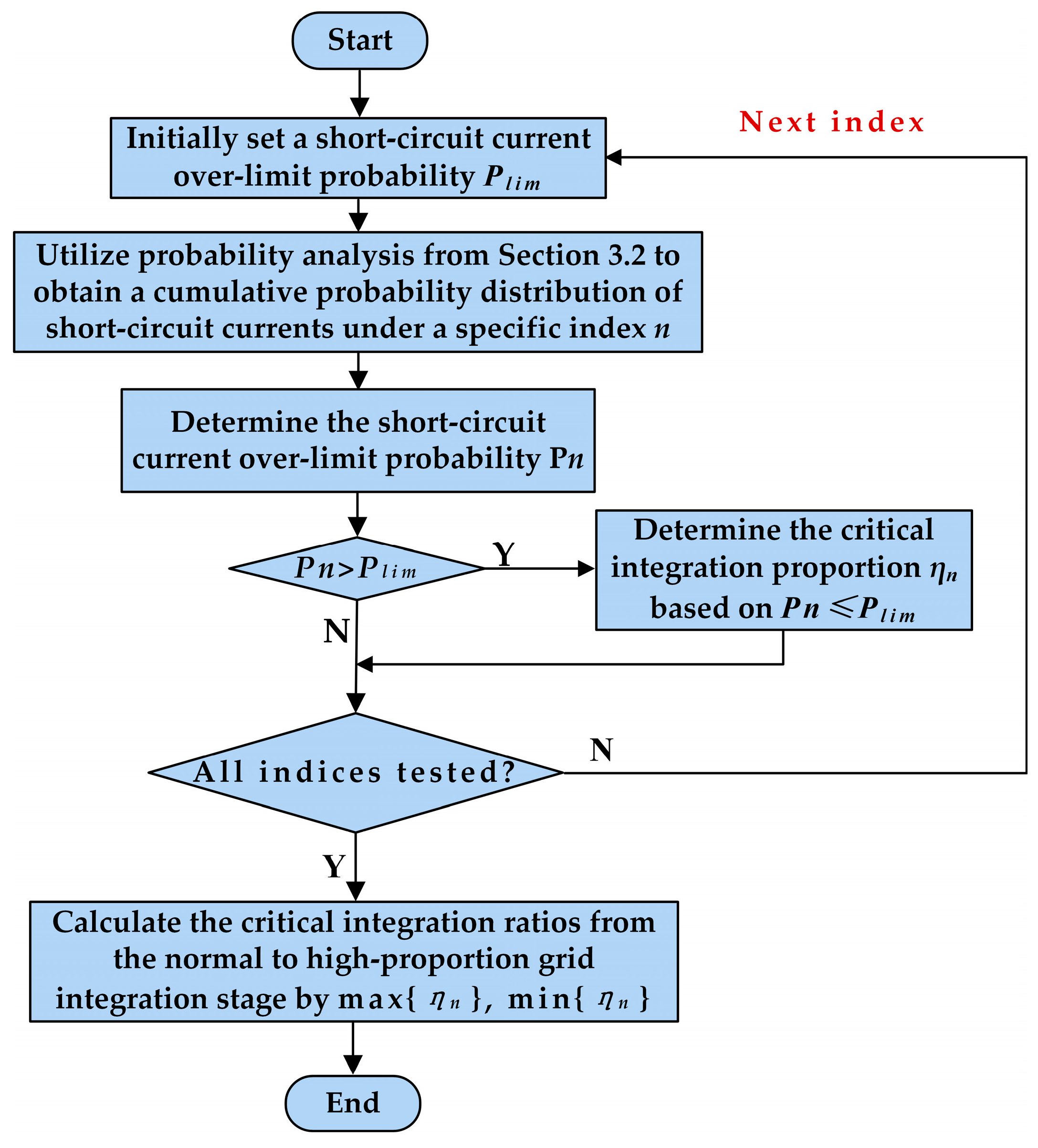
3.3. Calculation Method of Critical Integration Proportion of Inverter-Based Power Sources under High-Ratio Stage

The increasing proportion of the inverter-based power source integration has various impacts on the power system. Establishing the principles for categorizing different stages during the high proportion grid integration of inverter-based power sources can enhance the description and understanding of its effects on the power system. Therefore, the principles based on the operational risk assessment of the power system after grid integration of inverter-based power sources are proposed for categorizing these different grid integration stages for a high proportion of grid-connected inverter-based power sources.

This paper adopts a probabilistic and statistical approach to categorization, considering that the system enters the high-proportion stage of inverter-based power source integration when the exceeding probability of the system short-circuit current surpasses a threshold P_lim. P_lim is determined by the potential societal and economic losses resulting from the short-circuit current over-limit, and it is considered as the ratio of tolerable losses to the losses incurred from the short-circuit current over-limit. The five evaluative indices, SCCBFP, EDSFP, ETSFP, CSHTOP, and RCIMSOP, proposed in this paper, aim at assessing the operational risk to the system’s switching devices and conductors. Due to differing assessment methodologies, the grid integration proportion of inverter-based power sources corresponding to the probabilities of exceeding P_lim assessed by the different indices may vary. Therefore, a critical region (A, B) from a normal to a high proportion is defined as

$$\left\{\begin{array}{l}A=\min \left\{{\eta }_{SCCBFP},{\eta }_{EDSEP},{\eta }_{ETSEP},{\eta }_{CSHTOP},{\eta }_{RCIMSOP}\right\}\\ B=\max \left\{{\eta }_{SCCBFP},{\eta }_{EDSEP},{\eta }_{ETSEP},{\eta }_{CSHTOP},{\eta }_{RCIMSOP}\right\}\end{array}\right.$$

(19)

This critical region enables a stage categorization of the inverter-based power source integration proportion. Through this transitional critical area, the system enters the high-proportion stage of inverter-based power source grid integration, as illustrated in Figure 5.

The overall steps for calculating the high-proportion integration ratio of inverter-based power sources based on the risk assessment of short-circuit exceeding current limits are shown in Figure 6 and summarized as follows:

• Initially, set a short-circuit current over-limit probability P_lim for the high-proportion grid integration stage of the inverter-based power source.
• Utilize probability analysis from Section 3.2 to obtain a cumulative probability distribution [31] of short-circuit currents. Combine this with the maximum safe short-circuit current under a specific index to determine the short-circuit current over-limit probability P_n.
• Compare the high-proportion exceedance probability P_lim with the short-circuit current over-limit probability P_n to determine the critical integration proportion under the assessment criteria of a certain index constraint.
• Calculate the critical integration ratios from the normal- to high-proportion stage for inverter-based power sources under the assessment criteria of SCCBFP, EDSFP, ETSFP, CSHTOP, and RCIMSOP. The critical integration region is then defined by the maximum and minimum values of these critical proportions.

4. Case Study

4.1. Basic Data

In this case study, the proposed operational risk evaluation framework is validated based on a 220 kV level power system with inverter-based power sources in the middle area of China. The grid structure is depicted in Figure 7. The simulation is based on the actual equipment parameters and five years of fault data of the studied 220 kV system. The fault data include the specific line of each fault and its location within the line. The simulation model is developed in MATLAB/Simulink [32] to demonstrate the effectiveness of the proposed model through simulation analysis and calculations. Simscape [33] within MATLAB/Simulink offers readily available models for simulations in power systems and power electronics. By leveraging the physical connections of the studied system, relevant models can be directly constructed. With fault information set according to sampling, fault simulations can also be conducted efficiently.

According to the statistical data, the total installed capacity of photovoltaic (PV) generation in this region is 894 MW, while the year’s maximum load is 2848 MW, resulting in a PV power installation proportion of 31.4%. According to the region’s plans for PV expansion, combined with the PV addition scheme proposed in this paper, while disregarding the impact of load growth, this case study carries out system fault simulation sampling at 31%, 35%, 50%, 60%, 70%, and 90%. The Monte Carlo sampling iteration M for each PV installation capacity proportion scenario is set as 350 based on the method in reference [34] and empirical trial and error. Therefore, A total number of 2100 fault sampling simulations are conducted, with each sampling yielding fault parameters under the respective fault conditions.

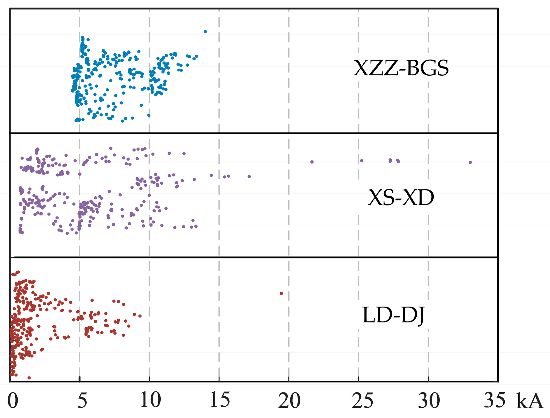
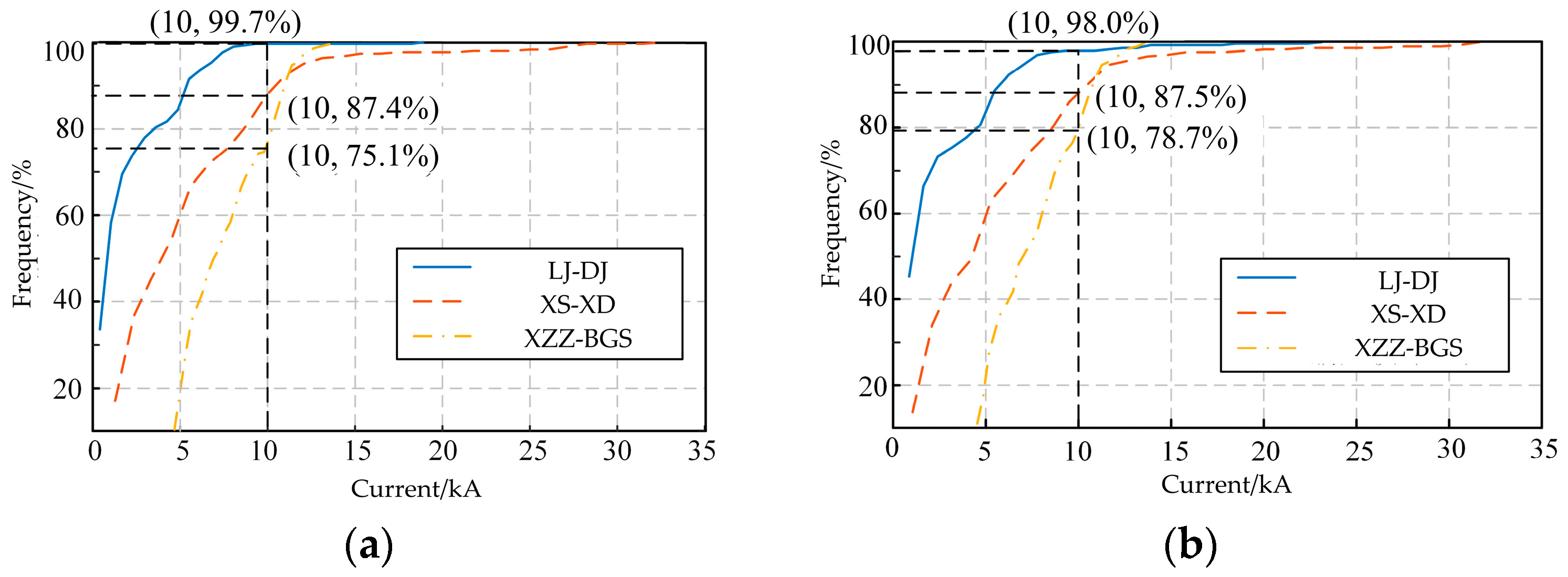
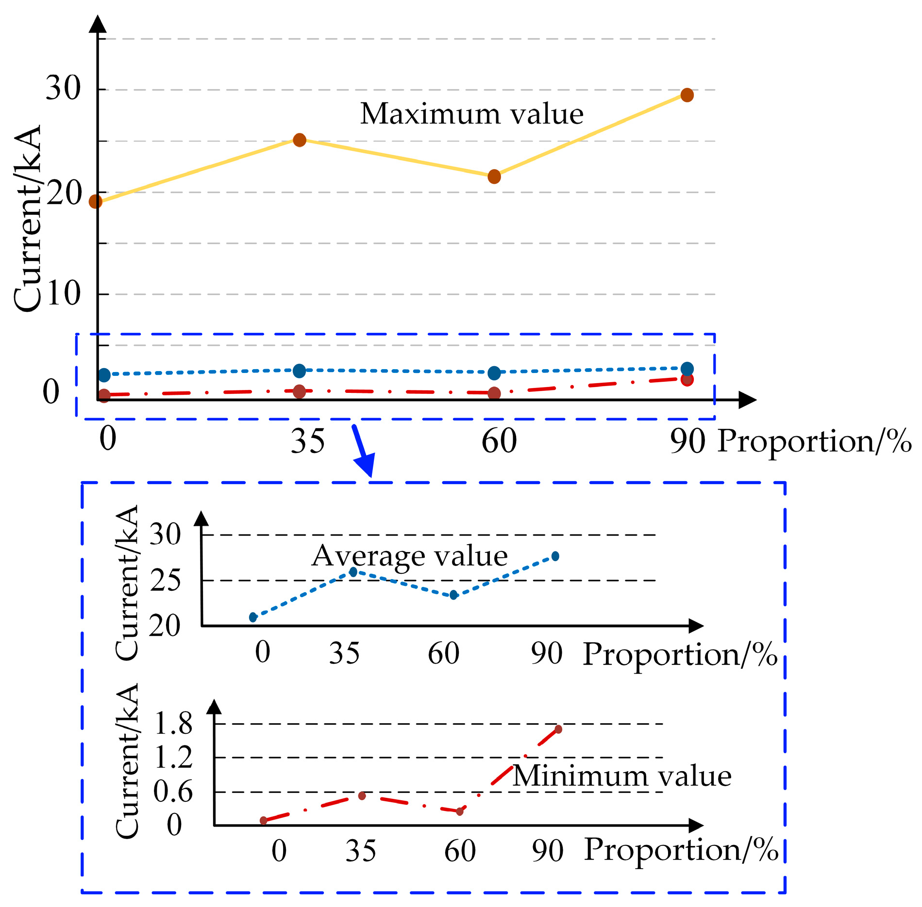
4.2. Short-Circuit Currents Analysis under Different Grid-Connection Scenarios of Inverter-Based Power Stations

By analyzing the fault data before the grid integration of inverter-based PV stations, the distribution of line short-circuit currents before grid connection can be obtained. Figure 8 shows the distribution of short-circuit impact currents for each fault sampling on the DJ-LJ, XS-XD, and XZZ-BGS lines within the studied power grid. The figure reveals that the background short-circuit current levels vary across different lines before the grid integration of inverter-based PV stations, leading to differences in the potential installed capacity for each station.

Figure 9a presents the cumulative probability distribution functions of fault currents for the three lines before the integration of PV stations into the power grid, while Figure 9b displays the cumulative probability distribution functions for the short-circuit impact currents after the integration of PV stations into the power grid, which can illustrate the changes in short-circuit current levels. From the figures, it is evident that the grid integration of PV stations has a minor impact on the fault current level of the XS-XD line, with the probability of exceeding 10 kA decreasing from approximately 12.6% to 12.5%. For the XZZ-BGS line, there is a noticeable reduction in the short-circuit current level, with the probability of exceeding 10 kA dropping from about 24.9% to 21.3%. Conversely, for the GQ-TZ line, there is a slight increase in the short-circuit current level, with the probability of exceeding 10 kA rising from approximately 0.3% to 2%. Therefore, differences in grid connection capacity caused by varying background short-circuit currents can affect the short-circuit current levels of lines after the grid connection of inverter-based power stations, potentially leading to increases, decreases, or stability of the short-circuit current over-limit probabilities.

The grid connection location of inverter-based power stations results in varying impacts on the system’s short-circuit current following a fault. According to the growth regulations for inverter-based power source installation capacity, the grid connection proportion of inverter-based power sources increases from 0% to 35% through proportional capacity expansion at existing stations, from 35% to 70% through proportional capacity expansion at four newly constructed stations, and beyond 70% through proportional capacity expansion at all stations. Figure 10 illustrates the trend of the short-circuit impact current on the DJ-LJ line as the grid connection proportion of inverter-based power sources increases. The figure shows that the short-circuit current level increases as the installed capacity at existing stations grows to a proportion of 35%. When the installed capacity begins to increase at new stations, the short-circuit current level tends to decrease. Finally, when all stations expand their installed capacity to a proportion of 90%, the short-circuit current level rises again. Therefore, the grid connection location of inverter-based power stations in the system directly affects the magnitude of the line’s short-circuit current level.

The impact of inverter-based power sources on system short-circuit currents varies with their grid connection ratio. Among 2100 fault-sampling data, the statistical diagram of the system short-circuit currents under different installed capacity ratios of PV is illustrated in Figure 11. Figure 11a uses the minimum, average, and maximum values to describe the level of short-circuit currents, with blue markers indicating maximum values, orange for average values, and green for minimum values. Each arrow corresponds to the short-circuit current for a specific proportion. Figure 11b shows the probability distribution of system short-circuit currents from a 31% to 90% integration ratio. The diagrams reveal that as the grid integration ratio of inverter-based power sources increases, so does the level of system short-circuit currents, which could potentially impact the operational safety of the system at certain ratios, underscoring the need for an assessment of the system’s operational risks.

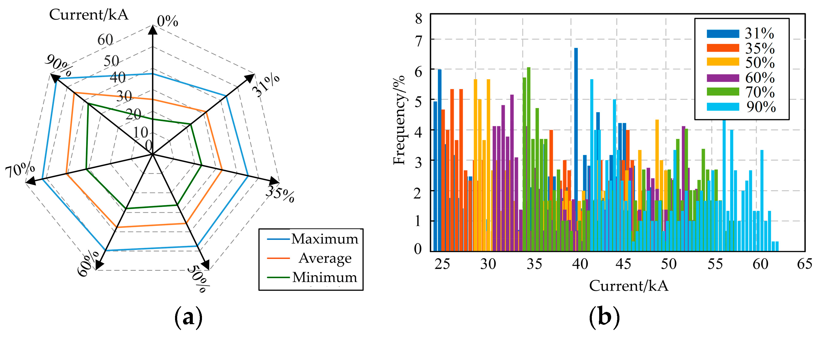
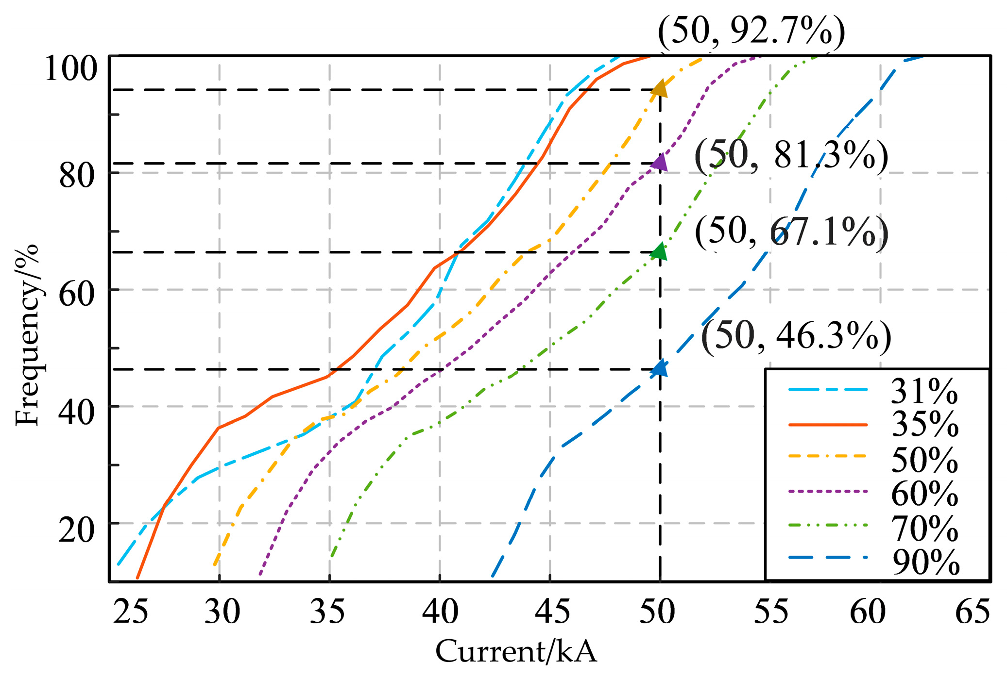
4.3. Calculation of Critical Integration Proportion of Inverter-Based Power Sources under High-Ratio Stage

From the analysis above, it is evident that as the grid integration ratio of inverter-based power sources increases, the system short-circuit currents level continuously rises, potentially causing damage to existing electrical equipment. Based on the operational risk evaluation indices of the power system, this paper considers that reaching an exceedance probability of 20% or above for any indices signifies the high-ratio stage. Due to the variation in the models of line equipment within the system, each equipment has different safe operational parameters. To make the conclusions more referenceable, the evaluation is conducted using fault sampling data for short-circuit currents on lines with identical equipment models, with parameters as shown in

Table 2. Parameters of circuit breaker.

Parameter	Value
Model	LW53-252/3150
Rated voltage/kV	252
Rated current/kA	3150
Rated breaking current/kA	50
Dynamic stability current/kA	125
Thermal stability current/kA·s−1	50/4

.

The SCCBFP index is assessed through the probability distribution for the RMS value of system short-circuit currents. Figure 12 shows the cumulative probability distribution function of system short-circuit currents under different grid integration ratios. The figure reveals that with increasing integration ratios, the probability of short-circuit current levels exceeding 50 kA increases. When the integration ratio of inverter-based power sources is below 35%, there is a high probability that short-circuit current interruption failure will not occur. At the 50% ratio, the probability of such failure is about 7.3%; when the ratio exceeds 60%, the failure probability exceeds 18.7%. Given that P_lim = 20%, it is considered that reaching an integration ratio of about 60% for inverter-based power sources marks the threshold of the high-ratio stage.

The selected model of a high-voltage circuit breaker can maintain dynamic and thermal stability during system fault conditions. Although high-voltage disconnect switches do not require verification for breaking current, they require checks for thermal and dynamic stability. The parameters for the disconnector are as shown in

Table 3. Parameters for disconnector.

Parameter	Value
Model	GW4-220D/1000
Rated voltage/kV	220
Rated current/kA	1000
Dynamic stability current/kA	80
Thermal stability current/kA·s−1	21.5/5

.

The index EDSFP is evaluated through the probability distribution of system short-circuit impulse currents. Figure 13 shows the cumulative probability distribution function of system impulse currents at different grid integration ratios. According to the diagram, dynamic stability is likely maintained when the ratio is below 60%. At the 70% integration ratio, the failure probability is approximately 10%, while at the 90% integration ratio, the probability rises to about 35%. Based on the trend of the distribution, it can be estimated that the high proportion stage is reached when the grid integration ratio of inverter-based power sources is around 80%.

The assessment of the ETSFP index relates to the moments when the short-circuit current RMS value reaches its maximum at time t₁ and when the current stabilizes at time t₂. Figure 14 shows the probability distribution for the occurrence times of the short-circuit impulse current and the maximum short-circuit current RMS value. Theoretically, the short-circuit impulse current should appear about half a cycle after the fault occurs [35] with a system frequency f = 50 Hz, indicating the impact current should appear at 0.01 s. As shown in Figure 14a, the highest probability of the impulse current appears at 0.009 s, with each fault sampling occurring within an error margin of 0.001 s, demonstrating that the simulation results are in line with theoretical expectations. Consequently, Figure 14b indicates that the peak of the short-circuit current RMS value occurs around 0.023 s. Similarly, the moment of stabilization is estimated to be around 0.13 s.

The maximum allowable short-time heating for the disconnector is 21.5² × 5 = 2311.25 kA²·s. The cumulative probability distribution function for short-time heating of the short-circuit current for each grid integration ratio calculated using the data from each sampling and Equation (4) is shown in Figure 15. From the figure, it is evident that thermal stability is likely to be maintained even when the installed capacity ratio reaches 90%, indicating that this metric does not impose constraints on categorizing different stages for inverter-based power source grid integration in this test system.

When assessing the operational risk for conductors, to ensure that the evaluation results are consistent across the same grid connection ratios, the maximum value of the line short-circuit current levels for each fault sampling is chosen from all lines with the same model of equipment. The parameters of the conductors are described in

Table 4. Parameters of conductor.

Parameter	Value
Model	JL/G1A-300/4
Calculated total cross-sectional area/mm2	338.99
Conductor outer diameter/mm	23.9
Weight per unit length/kg·km−1	1131
Calculated breaking force/N	92360
Elastic modulus/N/mm2	73000
Coefficient of linear expansion/×10−6·°C−1	19.6
DC resistance at 20 °C·Ω−1·km−1	0.0961

.

The assessment of the CSHTOP index is related to the conductor’s cross-sectional area. Substituting sampling data into Equation (9), since K_j is less than one for this system, it can be omitted in the calculation. Referring to the electrical design manual, the C value at the maximum allowable temperature of +70 °C is 67. This allows the calculation of the cumulative probability distribution function for the equivalent cross-sectional area of the conductor’s short-time heating at various integration ratios, as shown in Figure 16. The diagram indicates that at the installation ratio of 90%, the conductor short-term heating temperature over-limit probability is low. Therefore, this index does not impose a constraint on categorizing different stages of inverter-based power source grid integration for this test system.

Bus conductor parameters are outlined in

Table 5. Parameters of bus.

Parameter	Value
Material	Aluminum–manganese alloy tube
Conductor size D1/D2/mm	Φ100/90
Conductor cross-sectional area/mm2	1491
Current carrying capacity at maximum allowable temperature of +70 °C/A	2350
Section modulus/cm3	33.8
Radius of gyration/cm	3.36
Moment of inertia/cm⁴	169
Phase-to-phase distance/m	3
Span length/cm	1300
Allowable stress of material/N·cm−2	8820

. Substituting the system short-circuit impulse currents from each fault sampling into Equations (6) and (7), the cumulative probability distribution function for the maximum stress generated in rigid conductors by system short-circuit impulse currents at various integration ratios is shown in Figure 17. According to the figure, at the installed capacity ratio of 90%, the probability of the maximum stress induced by system short-circuit impact currents exceeding 2400 N/cm² is low, remaining below the material’s allowable stress. Therefore, this index also does not restrict the categorization of integration stages for inverter-based power sources in this test system.

To sum up, for the studied system in this case study, the operational risk assessment shows that the SCCBFP and EDSFP indices play a major role in the calculation of the critical integration proportion of inverter-based power sources. The critical integration ratios from the normal- to high-proportion stage for inverter-based power sources of the studied system range from 60% to 80%. Compared to existing studies that calculate PV hosting capacity based on steady-state operational conditions [36], the proposed short-circuit current over-limits probability-based approach accounts for the impact of short-circuit current impulse during faults on the system. Methods focusing solely on normal operational states may conclude that the maximum integration capacity of PV can exceed 100% [37], which fails to consider the potential risks associated with fault conditions.

5. Conclusions

This paper proposes an evaluation model for calculating the critical integration proportion of grid-connected inverter-based power sources considering the short-circuit current over-limit probability. Through the case study, the results can be summarized as follows:

• An increase in the grid integration ratio of inverter-based power sources elevates the risks associated with the switchgear failing to interrupt short-circuit currents, dynamic and thermal stability failures, as well as conductor heating and instantaneous stress over-limits during short-circuits.
• Evaluating the operational risks of the power system from a probabilistic perspective based on the inverter-based power source integration proportion provides a more objective approach compared to analyses that focus solely on specific scenarios. Through the evaluation, a more comprehensive basis for station planning and equipment selection can be obtained.
• The calculation of critical integration proportion categorization of inverter-based power sources from normal to high proportion stages shows that the baseline short-circuit current level, grid connection locations of inverter-based power stations, and the grid integration ratio of inverter-based power sources all significantly influence the system short-circuit current level. The dynamic stability and thermal stability of the equipment significantly influence the critical integration ratio of inverter-based power sources.

References

1. Yu, B.; Fang, D.; Xiao, K.; Pan, Y. Drivers of renewable energy penetration and its role in power sector’s deep decarbonization towards carbon peak. Renew. Sustain. Energy Rev. 2023, 178, 11237. [Google Scholar] [CrossRef]
2. Li, Y.; Zou, Y.; Tan, Y.; Cao, Y.; Liu, X.; Shahidehpour, M.; Tian, S.; Bu, F. Optimal stochastic operation of integrated low-carbon electric power, natural gas, and heat delivery system. IEEE Trans. Sustain. Energy 2017, 9, 273–283. [Google Scholar] [CrossRef]
3. Tan, L.; Yang, J.; Zhou, C. Historical review and synthesis of global carbon neutrality research: A bibliometric analysis based on R-tool. J. Clean. Prod. 2024, 449, 141574. [Google Scholar] [CrossRef]
4. Liao, J.; Guo, C.; Zeng, L.; Kang, W.; Zhou, N.; Wang, Q. Analysis of residual current in low-voltage bipolar DC system and improved residual current protection scheme. IEEE Trans. Instrum. Meas. 2022, 71, 9006013. [Google Scholar] [CrossRef]
5. Hossain, M.; Abboodi Madlool, N.; Al-Fatlawi, A.; El Haj Assad, M. High Penetration of Solar Photovoltaic Structure on the Grid System Disruption: An Overview of Technology Advancement. Sustainability 2023, 15, 1174. [Google Scholar] [CrossRef]
6. Telukunta, V.; Pradhan, J.; Agrawal, A.; Singh, M.; Srivani, S.G. Protection challenges under bulk penetration of renewable energy resources in power systems: A review. CSEE J. Power Energy Syst. 2017, 3, 365–379. [Google Scholar] [CrossRef]
7. Wen, Y.; Yang, W.; Wang, R.; Xu, W.; Ye, X.; Li, T. Review and Prospect of toward 100% Renewable Energy Power Systems. Proc. CSEE 2020, 40, 1843–1856. [Google Scholar]
8. Pandi, V.R.; Zeineldin, H.H.; Xiao, W.; Zobaa, A.F. Optimal penetration levels for inverter-based distributed generation considering harmonic limits. Electr. Power Syst. Res. 2013, 97, 68–75. [Google Scholar] [CrossRef]
9. Bai, X.; Fan, Y.; Hou, J.; Liu, J. Evaluation method of renewable energy flexibility confidence capacity under different penetration rates. Energy 2023, 281, 128327. [Google Scholar] [CrossRef]
10. Kondziella, H.; Bruckner, T. Flexibility requirements of renewable energy based electricity systems–a review of research results and methodologies. Renew. Sustain. Energy Rev. 2016, 53, 10–22. [Google Scholar] [CrossRef]
11. Hosseinzadeh, N.; Aziz, A.; Mahmud, A.; Gargoom, A.; Rabbani, M. Voltage Stability of Power Systems with Renewable-Energy Inverter-Based Generators: A Review. Electronics 2021, 10, 115. [Google Scholar] [CrossRef]
12. Wu, Y.; Liu, D.; Liao, W.; Fan, Q. A continuous-time voltage control method based on hierarchical coordination for high PV-penetrated distribution networks. Appl. Energy 2023, 347, 121274. [Google Scholar] [CrossRef]
13. Marzooghi, H.; Garmroodi, M.; Verbič, G.; Ahmadyar, A.S.; Liu, R.; Hill, D.J. Scenario and sensitivity based stability analysis of the high renewable future grid. IEEE Trans. Power Syst. 2022, 37, 3238–3248. [Google Scholar] [CrossRef]
14. Fang, Y.; Jia, K.; Yang, Z.; Li, Y.; Bi, T. Impact of inverter-interfaced renewable energy generators on distance protection and an improved scheme. IEEE Trans. Ind. Electron. 2018, 66, 7078–7088. [Google Scholar] [CrossRef]
15. Cecati, F.; Zhu, R.; Liserre, M.; Wang, X. Nonlinear modular state-space modeling of power-electronics-based power systems. IEEE Trans. Power Electron. 2021, 37, 6102–6115. [Google Scholar] [CrossRef]
16. Zhang, Y.; Xie, L. A transient stability assessment framework in power electronic-interfaced distribution systems. IEEE Trans. Power Syst. 2016, 31, 5106–5114. [Google Scholar] [CrossRef]
17. Sun, J.; Zheng, Z.; Li, C.; Wang, K.; Li, Y. Optimal fault-tolerant control of multiphase drives under open-phase/open-switch faults based on DC current injection. IEEE Trans. Power Electron. 2021, 37, 5928–5936. [Google Scholar] [CrossRef]
18. Zhang, B.L.; Guo, M.F.; Zheng, Z.Y.; Hong, Q. Fault Current Limitation with Energy Recovery Based on Power Electronics in Hybrid AC-DC Active Distribution Networks. IEEE Trans. Power Electron. 2023, 38, 12593–12606. [Google Scholar] [CrossRef]
19. Northwest Electric Power Design Institute, Ministry of Water Resources and Electric Power. Handbook of Electrical Design for Power Engineering—Electrical Primary Part; China Electric Power Press: Beijing, China, 2018; pp. 231–379. [Google Scholar]
20. Shan, Y.; Ai, M.; Liu, W. Research on simulation calculation on short-circuit electrodynamics force of power transformer winding. Int. J. Appl. Electromagn. Mech. 2021, 65, 451–465. [Google Scholar] [CrossRef]
21. Jin, M.; Chen, W.; Xu, W.; Li, J.; Zhao, Y.; Zhang, Q.; Wen, T. A path of power transformers failure under multiple short-circuit impacts. Electr. Power Syst. Res. 2024, 229, 110216. [Google Scholar] [CrossRef]
22. Ametani, A.; Nagaoka, N.; Baba, Y.; Ohno, T.; Yamabuki, K. New Power System Transients: Theory and Applications; CRC Press: Boca Raton, FL, USA, 2016. [Google Scholar]
23. Yin, J.; Qian, W.; Huang, X. A New Short-Circuit Current Calculation and Fault Analysis Method Suitable for Doubly Fed Wind Farm Groups. Sensors 2023, 23, 8372. [Google Scholar] [CrossRef] [PubMed]
24. Denich, E.; Novati, P. Some notes on the trapezoidal rule for Fourier type integrals. Appl. Numer. Math. 2024, 198, 160–175. [Google Scholar] [CrossRef]
25. Riba, J.R.; González, D.; Bas-Calopa, P.; Moreno-Eguilaz, M. Experimental Validation of the Adiabatic Assumption of Short-Circuit Tests on Bare Conductors. IEEE Trans. Power Deliv. 2023, 38, 3594–3601. [Google Scholar] [CrossRef]
26. Oliveira, A.R.E.; Freire, D.G. Dynamical modelling and analysis of aeolian vibrations of single conductors. IEEE Trans. Power Deliv. 1994, 9, 1685–1693. [Google Scholar] [CrossRef]
27. Zou, Y.; Wang, Q.; Chi, Y.; Wang, J.; Lei, C.; Zhou, N.; Xia, Q. Electric load profile of 5G base station in distribution systems based on data flow analysis. IEEE Trans. Smart Grid 2022, 13, 2452–2466. [Google Scholar] [CrossRef]
28. Huang, R.; Qu, S.; Gong, Z.; Goh, M.; Ji, Y. Data-driven two-stage distributionally robust optimization with risk aversion. Appl. Soft Comput. 2020, 87, 105978. [Google Scholar] [CrossRef]
29. Yan, Z.; Zhao, T.; Xu, Y.; Koh, L.H.; Go, J.; Liaw, W.L. Data-driven robust planning of electric vehicle charging infrastructure for urban residential car parks. IET Gener. Transm. Dis. 2020, 14, 6545–6554. [Google Scholar] [CrossRef]
30. Fang, D.Z.; Jing, L.; Chung, T.S. Corrected transient energy function-based strategy for stability probability assessment of power systems. IET Gener. Transm. Dis. 2008, 2, 424–432. [Google Scholar] [CrossRef]
31. Ye, R.; Wang, H.; Tasarruf, B.; Zhang, Y. Fast and accurate method for short-circuit current calculation in distribution network with IIDGs. Int. J. Electr. Power Energy Syst. 2024, 155, 109622. [Google Scholar]
32. Simulink—Simulation and Model-Based Design—MATLAB. Available online: https://ww2.mathworks.cn/products/simulink.html (accessed on 16 March 2024).
33. Simscape—Model and Simulate Multidomain Physical Systems. Available online: https://ww2.mathworks.cn/products/simscape.html (accessed on 9 April 2024).
34. Arouna, B. Adaptative Monte Carlo Method, A Variance Reduction Technique. Monte Carlo Methods Appl. 2004, 10, 1–24. [Google Scholar] [CrossRef]
35. Jia, K.; Hou, L.; Liu, Q.; Fang, Y.; Zheng, L.; Bi, T. Analytical calculation of transient current from an inverter-interfaced renewable energy. IEEE Trans. Power Syst. 2021, 37, 1554–1563. [Google Scholar] [CrossRef]
36. Yuan, J.; Weng, Y.; Tan, C.W. Determining maximum hosting capacity for PV systems in distribution grids. Int. J. Electr. Power Energy Syst. 2022, 135, 107342. [Google Scholar] [CrossRef]
37. Umoh, V.; Davidson, I.; Adebiyi, A.; Ekpe, U. Methods and Tools for PV and EV Hosting Capacity Determination in Low Voltage Distribution Networks—A Review. Energies 2023, 16, 3609. [Google Scholar] [CrossRef]
Figure 1. Temporal variation of short-circuit current RMS value (blue line: short-circuit current RMS value over fault duration).
Electronics 13 01486 g001
Figure 2. Schematic diagram of power system with inverter-interfaced power plants.
Electronics 13 01486 g002
Figure 3. Schematic diagram of the increase process in installed capacity of inverter-interfaced power plants.
Electronics 13 01486 g003
Figure 4. Flowchart of system operational risk probability evaluation.
Electronics 13 01486 g004
Figure 5. Schematic diagram of the development of the proportion of the grid-connected inverter-interfaced power source integration.
Electronics 13 01486 g005
Figure 6. Flowchart for the calculation of the high proportion grid integration of the inverter-interfaced power sources.
Electronics 13 01486 g006
Figure 7. Structure of the studied 220 kV power grid in the middle area of China.
Electronics 13 01486 g007
Figure 8. Scatter diagram of short-circuit impulse current on the three lines. (Note: The vertical dimension is expanded for visual clarity of closely spaced points and does not represent a specific scale.).
Electronics 13 01486 g008
Figure 9. Cumulative probability distribution diagram of the short-circuit impulse current on the three lines. (a) Before the PV integration; (b) after the 31% proportion of the PV integration.
Electronics 13 01486 g009
Figure 10. Trend of short-circuit impulse current in DJ-LJ line.
Electronics 13 01486 g010
Figure 11. Short-circuit current level and probability distribution of the system. (a) Short-circuit current level under integration proportion; (b) short-circuit current probability distribution under integration proportion.
Electronics 13 01486 g011
Figure 12. Cumulative probability distribution diagram for the RMS value of system short-circuit current.
Electronics 13 01486 g012
Figure 13. Cumulative probability distribution diagram of system short-circuit impulse current.
Electronics 13 01486 g013
Figure 14. Probability distribution of short-circuit impulse current and peak of RMS short-circuit current occurrence time. (a) Impulse current occurrence time; (b) peak RMS value occurrence time.
Electronics 13 01486 g014
Figure 15. Cumulative probability distribution diagram for the short-term heating of short-circuit current.
Electronics 13 01486 g015
Figure 16. Cumulative probability distribution of short-circuit current equivalent cross-sectional area.
Electronics 13 01486 g016
Figure 17. Cumulative probability distribution of stress generated by short-circuit impulse current.
Electronics 13 01486 g017