Model Predictive Control for Trajectory Planning Considering Constraints on Vertical Load Variation

Abstract

To address the issue of centrifugal force affecting the vertical load during the stability and trajectory planning of autonomous vehicles during high-speed cornering and obstacle avoidance, a model predictive control of trajectory planning and tracking is proposed that considers the roll factor using only a two-degrees-of-freedom vehicle dynamics model. Firstly, a trajectory planning controller is designed. As a predictive model, a dual-track two-degrees-of-freedom vehicle dynamics model is established. This model describes the relationship between tire lateral forces and vertical loads using a quadratic nonlinear tire model. To reflect the actual dynamic state of the vehicle, the controller incorporates a nonlinear constraint that considers vertical load variations. The nonlinear optimization problem is transformed into a simplified quadratic programming problem by using the Jacobian matrix method to linearize the constraints. By fitting a fourth-degree polynomial curve to the discrete points calculated by the replanning algorithm, an optimal collision-free trajectory is obtained. Secondly, an MPC trajectory tracking controller is designed to control the vehicle in real time along the optimal trajectory from the planning, incorporating control quantity constraints, control increment constraints, and lateral angle constraints to maintain the vehicle’s motion state. We transform the trajectory tracking control problem into a quadratic programming problem, solving for the optimal control sequence for the autonomous vehicle to track the trajectory, achieving an optimized solution and rolling time domain control. Finally, the effectiveness of the vehicle’s obstacle avoidance planning and tracking under high-speed double-lane-change maneuver conditions is validated using the Simulink simulation platform. The results indicate that the designed planning and tracking controllers effectively improve the obstacle avoidance planning and tracking control for high-speed autonomous vehicles.

1. Introduction

Autonomous driving technology, as one of the crucial innovations in the modern transportation sector, holds tremendous potential in enhancing traffic safety, reducing accidents, and improving traffic efficiency [1]. Trajectory planning, as one of the core aspects of autonomous driving technology, has attracted significant attention. To ensure the real-time safety [2] and stability of trajectory planning, scholars have conducted extensive research. More and more, trajectory planning is no longer limited to global trajectory planning, but also integrates local trajectory planning algorithms, including graph search methods [3], numerical optimization [4], interpolation [5], and sampling methods [6]. Compared to other methods of trajectory planning, the optimization-based model predictive control algorithm has advantages and limitations, as shown in

Table 1. Advantages and limitations of trajectory planning methods.

Trajectory Planning Methods	Advantages	Limitations
${\mathrm{A}}^{*}$ [7,8] and grid-based methods [9]	Low model requirements; fast calculation speed	Insufficient accuracy; limited scalability; large memory consumption
Model predictive control [10,11]	Real time; predictability; high accuracy; multi-constraint optimization; dynamic adaptability	High computational complexity; model uncertainty; difficulty in parameter adjustment
Online time-optimal trajectory planning [12]	Real time; accuracy; predictability; efficiency	Computational complexity draft; application scenario limitations; local optimal solution problem
Reinforcement learning [13,14]	Strong adaptability; suitable for complex environments	Large training data and resource requirements; possible convergence issues

.

Model predictive control, capable of multi-constraint multi-objective optimization control, is applicable to complex control problems involving multiple variables. When adopting model predictive control, the choice of the vehicle model in trajectory planning has an impact on computation, planning accuracy, and tracking effectiveness. To simplify calculations, it is common practice to use a point mass model or a simple vehicle single-track kinematic model and to neglect vehicle roll and pitch motion. For example, in [15], a point mass model is used for path planning and tracking control of the planned trajectory under different operating conditions, and the tracking accuracy is further improved. A simplified two-degrees-of-freedom single-track model based on vehicle kinematics is established in [16]. The MPC replanning algorithm is used for path planning, which reduces the computation time.

While using a simple vehicle model can reduce computation time, the effect of vehicle roll on the handling stability and dynamic characteristics of vehicles during high-speed operating, especially in turning conditions, is significant and cannot be ignored [17]. Therefore, in trajectory planning and tracking control, it is essential to consider the roll dynamics in the modeling. Therefore, in [18], modifications are made based on the vehicle kinematic model to establish a nonlinear full-vehicle model with understeering characteristics. The planner based on this model enables the vehicle to avoid obstacles in a safer and more comfortable manner. In [19], the vehicle model considers roll factors, and model predictive control is applied to improve motion planning based on passive roll control, resulting in a better obstacle avoidance performance. In [20], road curvature and banking constraints are used to describe lateral and roll dynamics in the construction of a vehicle dynamics model. Multiple constraints are constructed in the design of the MPC controller. As a result, the optimal smooth path is obtained while satisfying the lateral dynamic stability and environmental constraints. It is evident that the effectiveness of obstacle avoidance can be improved by considering roll dynamics in vehicle modeling during path planning.

Many scholars also consider high-degree-of-freedom vehicle models in trajectory planning to meet the requirements of vehicle stability and safety. For example, in [21], addressing the optimal trajectory planning for autonomous vehicles, a six-degrees-of-freedom nonlinear vehicle model is established considering the influence of tire dynamics and roll motion. Numerical solution methods are applied for linearization to simplify calculations, ensuring obstacle avoidance effectiveness and enabling fast tracking of reference trajectories. Furthermore, the influence of off-road terrain on the stability and trajectory planning of autonomous vehicles is considered in [22]. An eight-degrees-of-freedom vehicle dynamics model is developed, and a local trajectory planning algorithm suitable for this problem is proposed, which improves both trajectory tracking performance and vehicle stability. A mixed-integer quadratic programming method is used for optimal trajectory planning in [23]. Linear model predictive control is applied for trajectory tracking using a 12-degrees-of-freedom vehicle model as a predictive model. The designed vehicle model is compared with the traditional kinematic model, a single-track model, and a complex high-fidelity multi-degree-of-freedom dynamic model to evaluate its performance. The study demonstrates the significant influence of pitch and roll angles on lateral acceleration. Therefore, considering high-degree-of-freedom vehicle models can improve obstacle avoidance planning and tracking performance.

Although considering the roll degree of freedom in the vehicle predictive model can accurately represent the vehicle’s dynamic characteristics, the model is complex, computationally intensive, and cannot guarantee real-time trajectory planning. In response to this dilemma, this paper proposes a solution for the high-speed operating conditions of autonomous vehicles by introducing model predictive control for trajectory planning and tracking using only a two-degrees-of-freedom vehicle dynamics model to account for roll factors. This model predictive control uses only a dual-track two-degrees-of-freedom vehicle dynamics model and employs a relatively simple quadratic nonlinear tire model to describe the relationship between vertical load and tire lateral forces. Constraints on the left and right vertical load variations are introduced into the cost function to express the vehicle roll dynamics problem in real time. Nonlinear constraint functions are linearized using the Jacobian matrix method for solving quadratic programming problems. The lateral acceleration is selected as the control variable for the planning controller, and the front wheel steering angle is selected for the tracking controller, facilitating trajectory planning and tracking control for the vehicle model. Finally, simulation is used to verify the effectiveness of the designed planning and control.

The innovation of this paper lies in proposing a trajectory planning and tracking model predictive control that considers roll factors using only a two-degrees-of-freedom vehicle dynamics model. The specific methods comprise the following two key points:

• A simple quadratic nonlinear tire model is introduced to describe the relationship between tire lateral force and vertical load;
• We incorporate consideration of the variation in vertical loads on the left and right sides of the vehicle into the controller design and integrate them into the constraints to represent the roll factor.

2. Dual-Track Dynamics Model

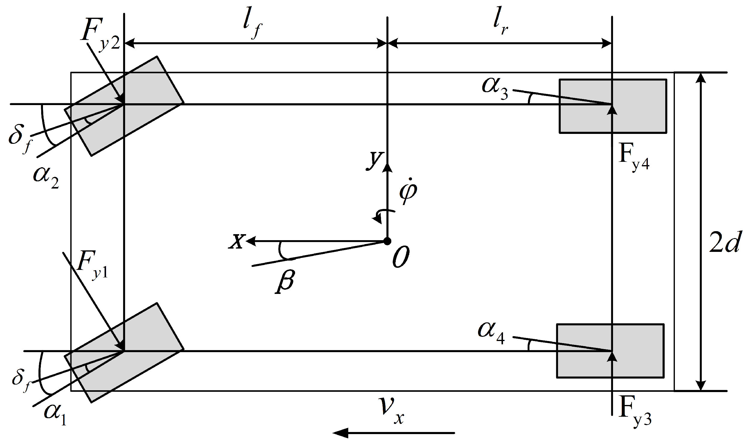
The dual-track two-degrees-of-freedom vehicle dynamic model is established as shown in Figure 1 and is used as the prediction model for model predictive control. The model uses a quadratic nonlinear tire model to express the relationship between vehicle vertical load, lateral deviation angle, and tire lateral forces.

When modeling vehicle dynamics, the motion characteristics of both longitudinal and lateral degrees of freedom are considered. In this model, the suspension is assumed to be rigidly connected to the chassis, neglecting the suspension motion and its effect on the coupling relationship. Due to the unpredictable and uncontrollable nature of real road conditions, the vehicle is assumed to be traveling on a flat road. Meanwhile, the influence of lateral and longitudinal aerodynamics on the vehicle’s yaw characteristics is disregarded due to computational complexity.

Based on the above description and assumptions, according to Newton’s second law of motion, we establish the equations of motion for the dual-track two-degrees-of-freedom vehicle dynamics to be as follows:

$$m\ddot{y}+m\dot{x}\dot{\phi }=F_{y1}+F_{y2}+F_{y3}+F_{y4}$$

(1)

$$I_z\ddot{\phi }=l_f(F_{y1}+F_{y2})-l_r(F_{y3}+F_{y4})$$

(2)

In Equations (1) and (2), m is the total vehicle mass; $\dot{y}$ is the lateral velocity of the vehicle center of mass; $\dot{x}$ is the longitudinal velocity of the vehicle center of mass; $\phi$ is the yaw angle of the vehicle; $\dot{\phi }$ is the yaw rate of the vehicle; $I_z$ is the yaw moment of inertia; $F_{yi}$ is the lateral force on the vehicle’s tires, where $i=1,2,3,4$; and $l_f$ and $l_r$ are the distances from the front and rear axles to the center of mass, respectively.

The lateral dynamic characteristics of a vehicle can be effectively described by including a tire model in vehicle modeling. Using the following quadratic tire empirical model [24], which can combine computational efficiency and practicality, the relationship between tire lateral force and vertical load can be expressed as:

$$F_{yi}=C_1{\alpha }_i{N}_i+C_2{\alpha }_i{N}_i^2,i=1,2,3,4$$

(3)

In the equation, $F_{yi}$ is the lateral force generated by the i-th tire, ${\alpha }_i$ is the side slip angle of the i-th tire, $N_i$ is the positive pressure on the tire, and $C_1$ and $C_2$ are empirical constants determined based on the tire experimental data.

Assuming that the lateral tire force is proportional to the small tire slip angle, and the value of the center of mass side slip angle $\beta$ is considered to be very small, the side slip angle ${\alpha }_i$ can be calculated using the following equation:

$$\begin{array}{c}{\alpha }_{1,2}=\beta +\frac{l_f\dot{\phi }}{\dot{x}}-{\delta }_f\hfill \\ {\alpha }_{3,4}=\beta -\frac{l_r\dot{\phi }}{\dot{x}}\hfill \end{array}$$

(4)

In the equation, ${\delta }_f$ is the front wheel steering angle.

The positive pressure $N_i$ on the four wheels, front and rear, left and right, can be expressed as:

$$\begin{array}{c}{N}_1=mg\frac{l_r}{2\left(l_f+l_r\right)}-\frac{l_r}{2d\left(l_f+l_r\right)}\left(m_{\mathrm{s}}{a}_{y}h\right)\hfill \\ N_2=mg\frac{l_r}{2\left(l_f+l_r\right)}+\frac{l_r}{2d\left(l_f+l_r\right)}\left(m_{\mathrm{s}}{a}_{y}h\right)\hfill \\ N_3=mg\frac{l_f}{2\left(l_f+l_r\right)}-\frac{l_f}{2d\left(l_f+l_r\right)}\left(m_{\mathrm{s}}{a}_{y}h\right)\hfill \\ N_4=mg\frac{l_f}{2\left(l_f+l_r\right)}+\frac{l_f}{2d\left(l_f+l_r\right)}\left(m_{\mathrm{s}}{a}_{y}h\right)\hfill \end{array}$$

(5)

In Equation (5), $m_s$ is the sprung mass of the vehicle, h is the distance from the vehicle center of mass to the roll axis, d is the half-track width, and $a_y$ is the lateral acceleration of the vehicle.

Additionally, geometric kinematic analysis can be used to obtain the approximate expression for the position of the vehicle, and the center of mass in the inertial coordinate system can be obtained as follows:

$$\begin{array}{c}\dot{Y}=\dot{x}sin\phi +\dot{y}cos\phi \hfill \\ \dot{X}=\dot{x}cos\phi -\dot{y}sin\phi \hfill \end{array}$$

(6)

In Equation (6), X and Y represent the position of the center of mass in the inertial coordinate system.

3. Design of Model Predictive Control Trajectory Planning Controller

In the design of the model predictive planning controller, the point mass model and the two-degrees-of-freedom model are simple but do not consider roll factors. On the other hand, multi-degree-of-freedom models considering roll factors are complex and computationally intensive. Here, a trajectory planning model predictive control is proposed that can consider the roll factor using only a two-degrees-of-freedom vehicle dynamics model.

3.1. Design of Obstacle Avoidance Function in Planner

Firstly, we design the obstacle avoidance function for each individual obstacle by adjusting the function value based on the distance deviation between the obstacle point and the target point. The closer the distance, the larger the function value. Considering the effect of vehicle speed and the weight of penalty functions in the objective function on obstacle avoidance, the following form of obstacle avoidance function is selected:

$${\mathrm{J}}_{obs,i}=\frac{S_{obs}{v}_i}{{(x_i-x_0)}^2+{(y_i-y_0)}^2+\rho }$$

(7)

Here, $\rho$ is the relaxation factor, set to 0.000001 to prevent division by zero in the denominator. $S_{obs}$ is the obstacle avoidance weight factor. ($x_i$, $y_i$) are the coordinates of the obstacle point with respect to the vehicle body coordinate system, while ($x_0$, $y_0$) are the coordinates of the vehicle’s center of mass.

3.2. Design of Planner’s Cost Function and Constraints

The control objective in the trajectory replanning layer is to minimize the deviation from the global reference path considering the condition of vertical load transfer, and to achieve obstacle avoidance.

Therefore, the designed cost function, including the obstacle avoidance function, control variables, and the global expected trajectory deviation for planned trajectory, is formulated as shown in the following equation:

$$\sum _{t=1}^{N_p}\left|\right|\eta \left(t+1|t\right)-{\eta }_{ref}{(t+1|t)\left|\right|}_Q^2+\left|\right|U_i{\left|\right|}_R^2+J_{obs,i}$$

(8)

In Equation (8), $N_p$ is the prediction time domain, ${\eta }_{ref}={[Y_{ref},{\phi }_{ref}]}^{\mathrm{T}}$ is the original reference trajectory, $\eta ={\left[Y,\phi \right]}^{\mathrm{T}}$ is the planned trajectory, the control variable is $U_i={\delta }_f$, and $J_{obs,i}$ is the obstacle avoidance function at sampling time i.

To compute a collision-free optimal trajectory that conforms to dynamic characteristics, constraints on the cost function need to be designed.

In cornering conditions, due to the effect of centrifugal force, the tire loads on the left and right sides are unequal, with the inner side being smaller and the outer side being larger. Since the tire lateral force and the vertical load have a nonlinear relationship, the inner tire lateral force decreases while the outer tire lateral force increases, resulting in an overall reduction of the lateral force [25]. In previous studies, constraints on the variation of lateral tire forces on both sides were not considered, resulting in a difference from actual conditions. Therefore, this paper constructs separate constraints for the left and right sides to reflect the actual relationship between the maximum lateral force and the vertical load as follows:

$$\begin{array}{c}{F}_{yl}\le \mu F_{zl}\hfill \\ F_{yr}\le \mu F_{zr}\hfill \end{array}$$

(9)

In the equation, $F_{yl}$ and $F_{yr}$ are the lateral forces of the left and right wheels, $\mu$ is the ground friction coefficient. Using Equation (5), the vertical loads on the left and right sides can be expressed as follows:

$$\begin{array}{c}{F}_{zl}=\frac{1}{2}mg-\frac{m{a}_{y}h}{2d}\hfill \\ F_{zr}=\frac{1}{2}mg+\frac{m{a}_{y}h}{2d}\hfill \end{array}$$

(10)

Furthermore, based on the balance of lateral tire forces and centrifugal force on the left and right sides, the following relationships are satisfied:

$$F_{yl}+F_{yr}=m{a}_y$$

(11)

From Equations (3), (9), (10), and (11), the nonlinear inequality constraints $c_1\left(x\right)$, $c_2\left(x\right)$ and the equality constraint $g_i\left(x\right)$ can be simplified to the following form:

$$\left\{\begin{array}{c}{c}_1\left(x\right)=C_1\left({\alpha }_1{N}_1+{\alpha }_3{N}_3\right)+C_2\left({\alpha }_1{N}_1^2+{\alpha }_3{N}_3^2\right)-\frac{1}{2}\mu mg+\frac{\mu m{a}_{y}h}{2d}\le 0,\hfill \\ c_2\left(x\right)=C_1\left({\alpha }_2{N}_2+{\alpha }_4{N}_4\right)+C_2\left({\alpha }_2{N}_2^2+{\alpha }_4{N}_4^2\right)-\frac{1}{2}\mu mg-\frac{\mu m{a}_{y}h}{2d}\le 0,\hfill \\ g_i\left(x\right)=C_1\left({\alpha }_1{N}_1+{\alpha }_3{N}_3\right)+C_2\left({\alpha }_1{N}_1^2+{\alpha }_3{N}_3^2\right)+C_1\left({\alpha }_2{N}_2+{\alpha }_4{N}_4\right)+\hfill \\ C_2\left({\alpha }_2{N}_2^2+{\alpha }_4{N}_4^2\right)-m{a}_y=0\hfill \end{array}\right.$$

(12)

The constraints that the cost function (8) must satisfy are shown in the above equation.

3.3. Linearization of Nonlinear Constraints

For practical constraints, solving for constraints is complicated by their nonlinear character; therefore, it is necessary to linearize the studied constraints. Linearizing nonlinear constraints greatly simplifies the solving process, and the Jacobian matrix method is used for linearization.

Firstly, based on Equation (12), we define the form of the inequality constraint function $c_j\left(x\right)$ as follows:

$$c_j\left(x\right)=\left\{\begin{array}{c}{c}_1\left(x\right)\hfill \\ c_2\left(x\right)\hfill \end{array}\right.$$

(13)

Secondly, we define the variable $x=[{\alpha }_i,N_i,a_y]$, where $i=1,2,3,4$, and the variable x is updated with the changing state at different times.

Additionally, to compute the function value of $c_j\left(x\right)$ at point $x^{*}$ and its gradient $\nabla c_j\left(x^{*}\right)$, we take partial derivatives with respect to each variable in the variable x. These derivative values will form the vectors of each row of the Jacobian matrix.

Thus, we construct the Jacobian matrix $A_n$ composed of gradient vectors, as shown in Equation (14).

$$A_n=\left[\begin{array}{c}\nabla c_1{\left(x\right)}^{\mathrm{T}}\hfill \\ \nabla c_2{\left(x\right)}^{\mathrm{T}}\hfill \end{array}\right]$$

(14)

$$\nabla c_1{\left(x\right)}^{\mathrm{T}}=\left[\begin{array}{ccc}\frac{\partial c_1}{\partial {\alpha }_i}& \frac{\partial c_1}{\partial N_i}& \frac{\partial c_1}{\partial a_y}\end{array}\right],i=1,2,3,4$$

(15)

$$\nabla c_2{\left(x\right)}^{\mathrm{T}}=\left[\begin{array}{ccc}\frac{\partial c_2}{\partial {\alpha }_i}& \frac{\partial c_2}{\partial N_i}& \frac{\partial c_2}{\partial a_y}\end{array}\right],i=1,2,3,4$$

(16)

where $\nabla c_1{\left(x\right)}^{\mathrm{T}}$ and $\nabla c_2{\left(x\right)}^{\mathrm{T}}$ are the gradient vectors of each constraint, as expressed by Equations (15) and (16).

The final expression for the Jacobian matrix is as follows:

$${A_n}^T=\left[\begin{array}{cc}{C}_1{N}_1+2C_1{C}_2{N}_1{\alpha }_1& 0\\ C_1·N_3& C_1{N}_4+2C_2{N}_4{\alpha }_4\\ C_1{\alpha }_1+2C_2{{\alpha }_1}^2·N_1& 0\\ 0& C_1{\alpha }_2+2C_2{N}_2{{\alpha }_2}^2\\ C_1{\alpha }_3+2C_2{N}_3{{\alpha }_3}^2& 0\\ 0& C_1{\alpha }_4+2C_2{N}_4{{\alpha }_4}^2\\ \begin{array}{c}\left(C_1{\alpha }_1+2C_2{\alpha }_1{N}_1\right)\frac{\partial N_1}{\partial a_y}+\hfill \\ \left(C_1{\alpha }_3+2C_2{\alpha }_3{N}_3\right)\frac{\partial N_3}{\partial a_y}+\frac{\mu mh}{d}\hfill \end{array}& \begin{array}{c}\left(C_1{\alpha }_2+2C_2{\alpha }_2{N}_2\right)\frac{\partial N_2}{\partial a_y}+\hfill \\ \left(C_1{\alpha }_4+2C_2{\alpha }_4{N}_4\right)\frac{\partial N_4}{\partial a_y}-\frac{\mu mh}{d}\hfill \end{array}\end{array}\right]$$

(17)

In solving quadratic programming problems, the inequality constraint is $c_j\left(x\right)\le 0$, which we linearize as:

$$c_j\left(x\right)\approx c_j\left(x_k\right)+A_n\left(x_k\right)\left(x-x_k\right)$$

(18)

In Equation (18), $x_k$ is the current iteration solution, and $A_n\left(x_k\right)$ is the Jacobian matrix of $c_j\left(x\right)$ at $x_k$.

Similarly, for the nonlinear equality constraint $g_i\left(x\right)$ in Equation (12), the linearization process is as described above.

3.4. Controller Solving

For the constrained optimal control problem of the MPC trajectory planning controller, obtaining its analytical optimal solution is difficult. Therefore, it can be reduced to solving the following quadratic programming problem, where $f,g,c$ represent the cost function, equality constraints, and inequality constraints, respectively:

$$\begin{array}{c}\underset{x\in R^n}{min}f\left(x\right)\hfill \\ \begin{array}{cc}{g}_i\left(x\right)=0& i=1,2,\end{array}\cdots ,m_p\hfill \\ \begin{array}{cc}{c}_j\left(x\right)\le 0& j=\end{array}{m}_p+1,\cdots ,m\hfill \end{array}$$

(19)

Constrained nonlinear programming is solved using quadratic programming (QP). It requires solving several QP subproblems to obtain the optimal solution of the original problem. Let $x_k$ be the current iteration solution, and solve the following QP subproblem:

$$\begin{array}{c}\underset{d\in R^n}{min}\frac{1}{2}{d}^T{B}_{k}d+\nabla f{\left(x_k\right)}^{T}d\hfill \\ \nabla g{\left(x_k\right)}^{T}d+g\left(x_k\right)=0\hfill \\ \nabla c{\left(x_k\right)}^{T}d+c\left(x_k\right)\le 0\hfill \end{array}$$

(20)

Assuming $d_k$ is the solution of Equation (20), using $d_k$ as the line search direction, and obtaining the step length $l_k$ through this search, the iteration point at time $k+1$ is $x_{k+1}=x_k+l_k{d}_k$. The gradients of $f,g,c$ at point $x_k$ are represented by $\nabla f\left(x_k\right)$, $\nabla g\left(x_k\right)$, $\nabla c\left(x_k\right)$, and $B_k$ is a positive definite matrix obtained from the weight matrices Q and R.

Finally, the quadratic programming problem is simplified to the following minimization problem:

$$\begin{array}{c}\underset{d\in R^n}{min}\frac{1}{2}{d}^T{B}_{k}d+q^{T}d\hfill \\ A_{n}d-b\le 0\hfill \\ \nabla g{\left(x_k\right)}^{T}d+g\left(x_k\right)=0\hfill \end{array}$$

(21)

Problem (21) always has an optimal solution $d_k$, $A_n$ is given by Equation (14), b is the upper bound value at the constraint points, $q={[0,0,S_{obs}]}^{\mathrm{T}}$, and S is the obstacle avoidance weight factor.

Additionally, in the trajectory replanning algorithm, the planned trajectory is provided as discrete points in the predicted time domain using a highly accurate fourth-degree polynomial for curve fitting. The planning layer and control layer are integrated to achieve the vehicle’s real-time tracking of the locally replanned desired trajectory.

4. Design of Model Predictive Control Trajectory Tracking Controller

An MPC trajectory tracking controller is designed based on the dual-track two-degrees-of-freedom dynamic model. A linear time-varying model predictive control is used, the nonlinear dynamic model is linearized, and a state-space model is established.

The system of equations can be written as:

$$\left\{\begin{array}{c}{\dot{\xi }}_{dyn}\left(t\right)=f\left({\xi }_{dyn}\left(t\right),u\left(t\right)\right)\hfill \\ y\left(t\right)=C{\xi }_{dyn}\left(t\right)\hfill \end{array}\right.$$

(22)

where ${\xi }_{dyn}={[\dot{y},\phi ,\dot{\phi },X,Y]}^{\mathrm{T}}$ is the state variable, $u={\delta }_f^{\prime }$ is the control variable, $y={[Y,\phi ]}^{\mathrm{T}}$ is the system output, and C is the identity matrix.

To ensure real-time control, the following objective function is established:

$$J({\xi }_{dyn}\left(t\right),u_{dyn}\left(t-1\right),\Delta U_{dyn}\left(t\right))=\sum _{i=1}^{N_p}∥y\left(t+i\left|t\right.\right)-{y_{dyn}\left(t+i\left|t\right.\right)∥}_Q^2+\sum _{i=1}^{N_c-1}{∥\Delta u_{dyn}\left(t+i\left|t\right.\right)∥}_R^2+\rho {\epsilon }^2$$

(23)

where $y_{dyn}=[Y_{ref},{\phi }_{ref}]$ is the input variable, and the expected output $y_{ref,local}={[Y_{local},{\phi }_{local}]}^{\mathrm{T}}$ is provided by the planning controller, where $Y_{local}$ and ${\phi }_{local}$ are the desired lateral position and yaw angle, respectively.

In addition, constraints are defined, including constraints on control variables and control increments, output constraints, and state constraints. These constraints are used to limit the trajectories generated during the optimization process, ensuring their feasibility and meeting the system’s performance requirements.

Therefore, constraints on front wheel steering angle and steering angle increment, vehicle yaw angle, and lateral displacement are defined as:

$$s.t.\left\{\begin{array}{c}-15\le {\delta }_f\le 15\left(\mathrm{deg}\right),\hfill \\ -0.8\le \Delta {\delta }_f\le 0.8\left(\mathrm{deg}\right),\hfill \\ -0.3\le \phi \le 0.35\left(\mathrm{rad}\right),\hfill \\ -3\le Y\le 5\left(\mathrm{m}\right)\hfill \end{array}\right.$$

(24)

These constraints are important reference criteria in the optimization process to obtain optimal and reasonable trajectory planning results.

Finally, the optimization function consisting of (23) and (24) is solved. Based on the two-degrees-of-freedom dynamic model, the MPC trajectory tracking controller needs to obtain the optimal solution in each control cycle.

At this point, the model predictive control problem can be transformed into solving a quadratic programming problem. At each sampling time t, by rolling through the time domain to solve the above optimization problem, the first element $u_{dyn}\left(t\right)$ of the optimal control sequence $\Delta U_{dyn,t}$ is used as the actual control input at the current time t, and the optimization process is repeated at the next sampling time $t+1$ to achieve tracking control of the desired trajectory.

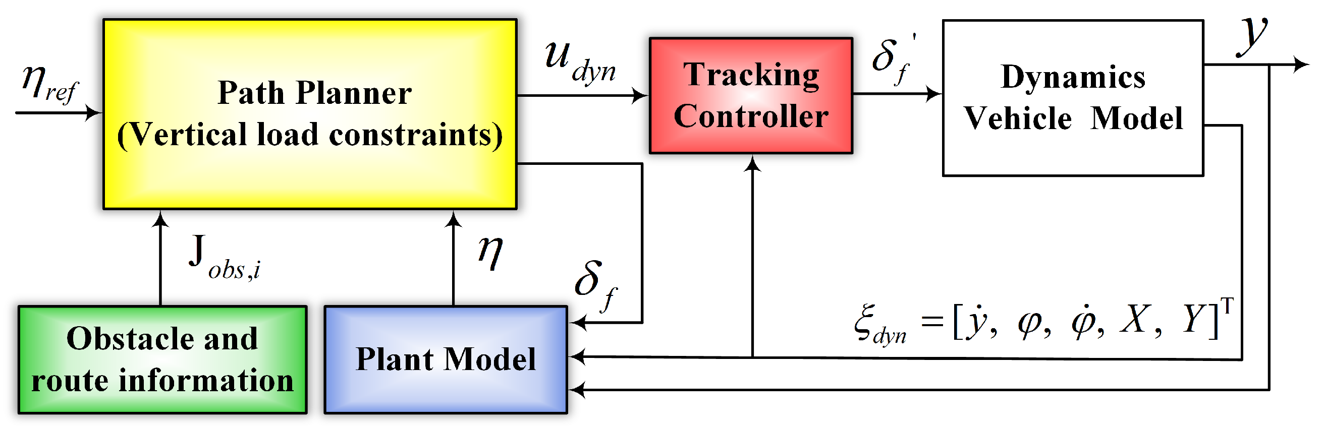
The two-layer trajectory planning, obstacle avoidance, and tracking system consists of the MPC trajectory planning controller and the tracking controller, as shown in the schematic diagram in Figure 2.

In Figure 2, firstly, nonlinear constraints considering vertical load variation are set in the upper-level trajectory planner. Based on the obstacle information detected by the vehicle sensors and the current vehicle state, the original expected path ${\eta }_{ref}={[Y_{ref},{\phi }_{ref}]}^{\mathrm{T}}$ is used as the actual input for the planner. Through MPC, the control quantity ${\delta }_f$ is adjusted in real time and input into the planning model for optimization. Eventually, a locally replanned trajectory $\eta$ is obtained, forming a closed-loop control. The variable ${\xi }_{dyn}$ is the feedback of state variables output by the dual-track two-degrees-of-freedom model to both the tracking controller and the planning controller.

Figure 2. MPC trajectory planning and tracking control system schematic diagram.

Figure 2. MPC trajectory planning and tracking control system schematic diagram.

The updated reference trajectory $u_{dyn}$ from the upper-level planner is received in the lower-level tracking controller, processed by MPC rolling optimization, and the updated control quantity ${\delta }_f^{\prime }$ is fed back to the dual-track two-degrees-of-freedom vehicle model for iterative optimization, forming a closed-loop control. The final output of the system is shown as y.

5. Simulation and Analysis

To validate the effectiveness of the designed model predictive control trajectory planning and tracking controller that take into account the constraints of the vehicle’s vertical load variation, Simulink simulation experiments are designed to simulate and analyze the vehicle’s obstacle avoidance planning and tracking control. The implementation of MPC trajectory obstacle avoidance planning and tracking is achieved through the use of MATLAB’s S-Function. The double-lane-change maneuver trajectory is chosen as the desired trajectory for the vehicle’s movement. This desired trajectory is highly dependent on speed [26]; hence, simulations and comparative analysis are conducted at longitudinal speeds of 20 m/s and 30 m/s, respectively.

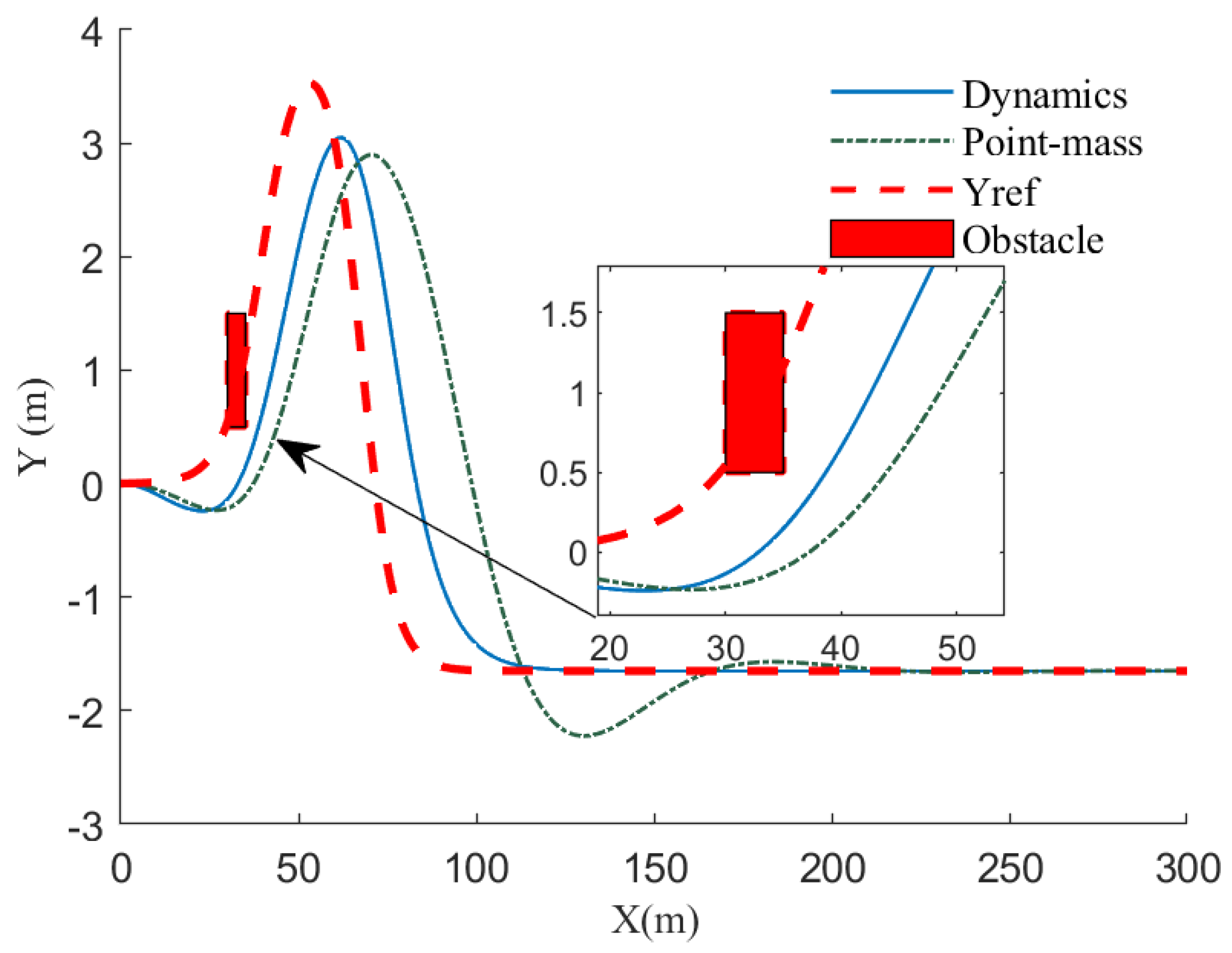
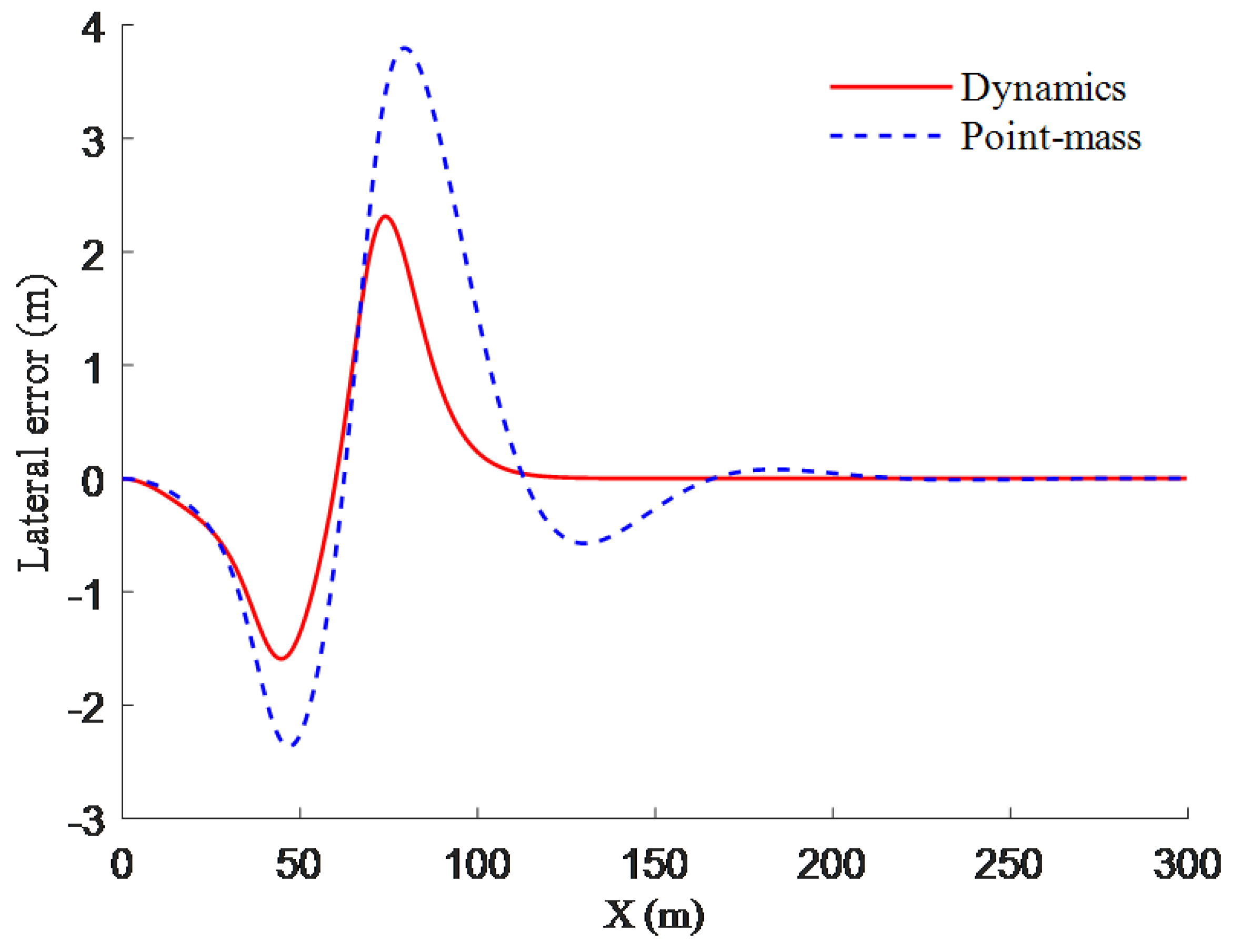
In the legend for all figures below, “Point-mass” denotes the MPC trajectory planner using a point mass model as the comparative planner; “Dynamics” represents the MPC trajectory planner with added nonlinear constraints, employing a dual-track two-degrees-of-freedom dynamic model as the predictive model, referred to as the “improved planner” in the following text; “Yref” stands for the original reference trajectory; “Obstacle” indicates the position information of obstacles, with obstacle coordinates set as (30, 0.5), (32.5, 0.5), (35, 0.5), (30, 1.5), (32.5, 1.5), and (35, 1.5) and the obstacles positioned on the double-lane-change maneuver trajectory. Additionally, the main parameters of the model are presented in

Table 2. Vehicle model parameters.

Parameter	Value	Parameter	Value
m (kg)	1740	$m_s$ (kg)	1500
$l_f$ (m)	1.4	$l_r$ (m)	1.7
h (m)	0.45	d (m)	0.75
$I_z$ (kg·m2)	2500	g (m·s−2)	9.8
$C_{cf}$ (N·rad−1)	76,339	$C_{cr}$ (N·rad−1)	70,351
$C_1$ (rad−1)	13.098	$C_2$ (N−1·rad−1)	−0.001045

[27].

5.1. Simulation of 20 m/s

Setting the vehicle speed to 20 m/s, initial position to (0, 0), ground friction coefficient $m_u$ to 0.8, simulation time to 10 s, and time step to 0.02 s, the simulation results are as illustrated in Figure 3, Figure 4, Figure 5, Figure 6 and Figure 7.

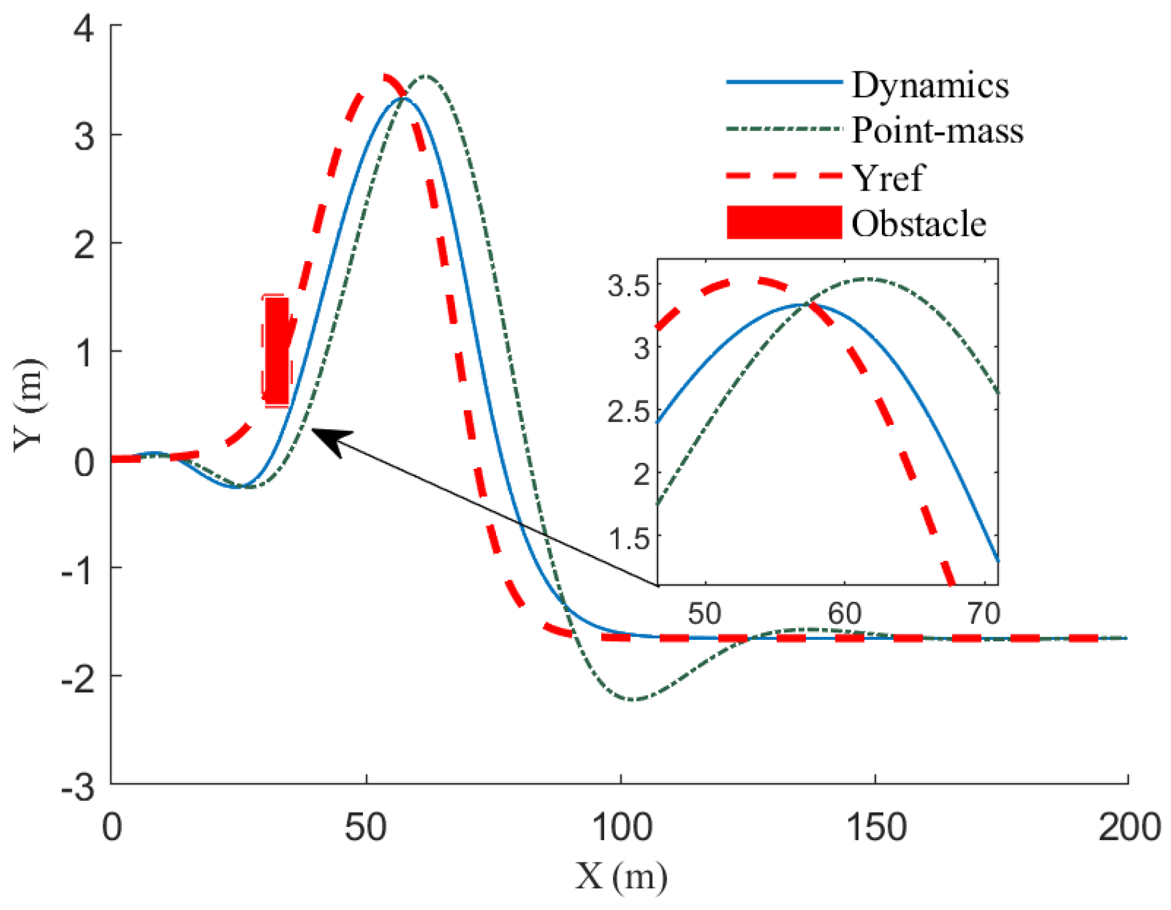
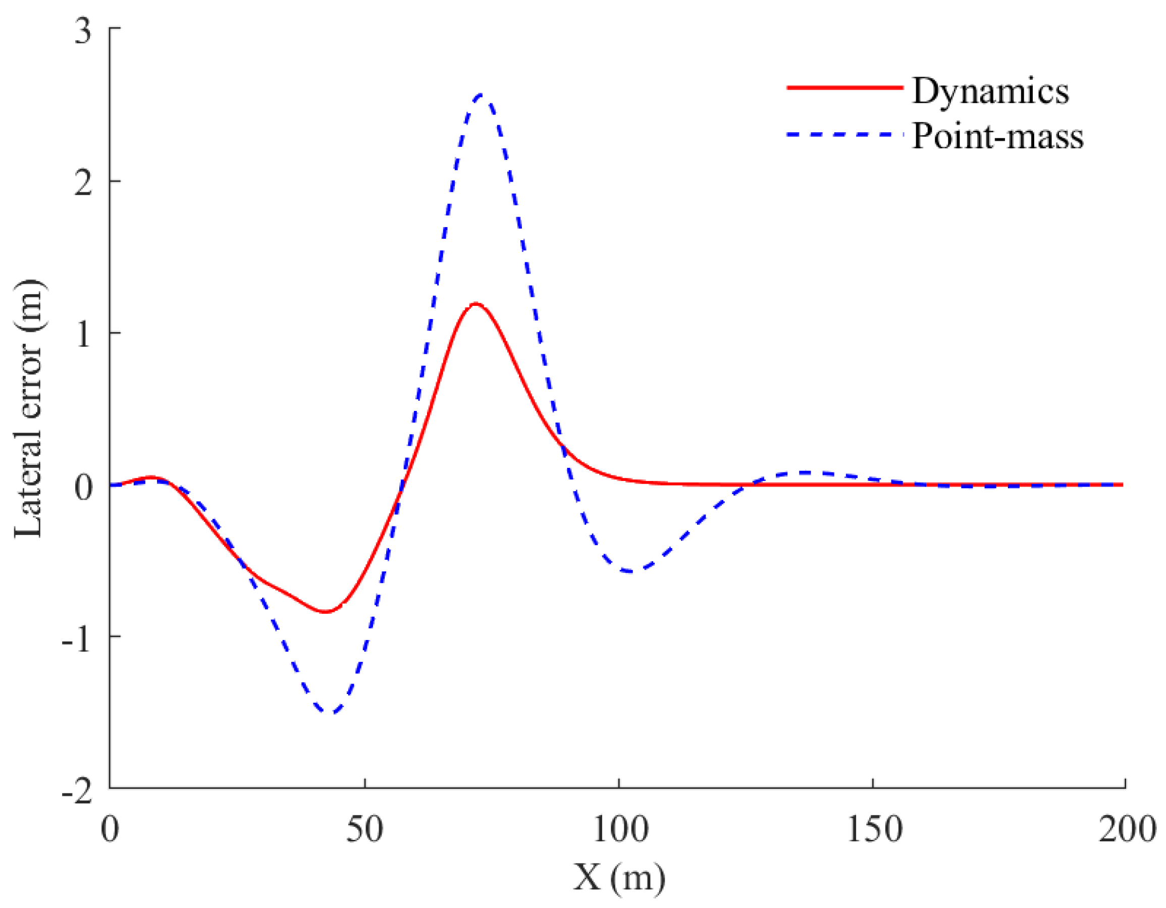
Figure 3 and Figure 4 depict the vehicle trajectory and lateral error diagram at a speed of 20 m/s, respectively. As can be observed from Figure 3, under the double-lane-change maneuver condition, the improved planner obtains a feasible trajectory at a speed of 20 m/s. It effectively accounts for obstacle avoidance, resulting in smoother vehicle trajectories at turns. After navigating the curve, the vehicle quickly approaches the desired trajectory. Examining the peak local magnification of Figure 3 and Figure 4, it is evident that the improved planner, after passing the highest point of the curve, exhibits a continuous reduction in lateral error. The maximum error is 1.19 m, which is 1.37 m less than the comparative planner, resulting in a 53.5% improvement in tracking performance at the curve. Figure 4 indicates that, during obstacle avoidance, the maximum lateral error for the comparative planner is 1.50 m, while the improved planner achieves a maximum lateral error of 0.83 m, a reduction of 44.7%. Furthermore, the lateral errors during obstacle avoidance are consistently lower for the improved planner compared to the comparative planner, improving the effectiveness of obstacle avoidance. At the curve where X = 100 m, the lateral error of the improved planner approaches zero, and the vehicle rapidly aligns with the reference trajectory, achieving quicker convergence to steady-state straight-line motion. In contrast, the lateral error of the comparative planner only approaches zero at X = 150 m, indicating better stability in the lateral error of the improved planner. As a result, the improved planner significantly outperforms the comparative planner in overall planning, obstacle avoidance, and tracking efficiency.

Figure 3. Comparison of the vehicle trajectories at 20 m/s.

Figure 3. Comparison of the vehicle trajectories at 20 m/s.

Figure 4. Comparison of lateral error at 20 m/s.

Figure 4. Comparison of lateral error at 20 m/s.

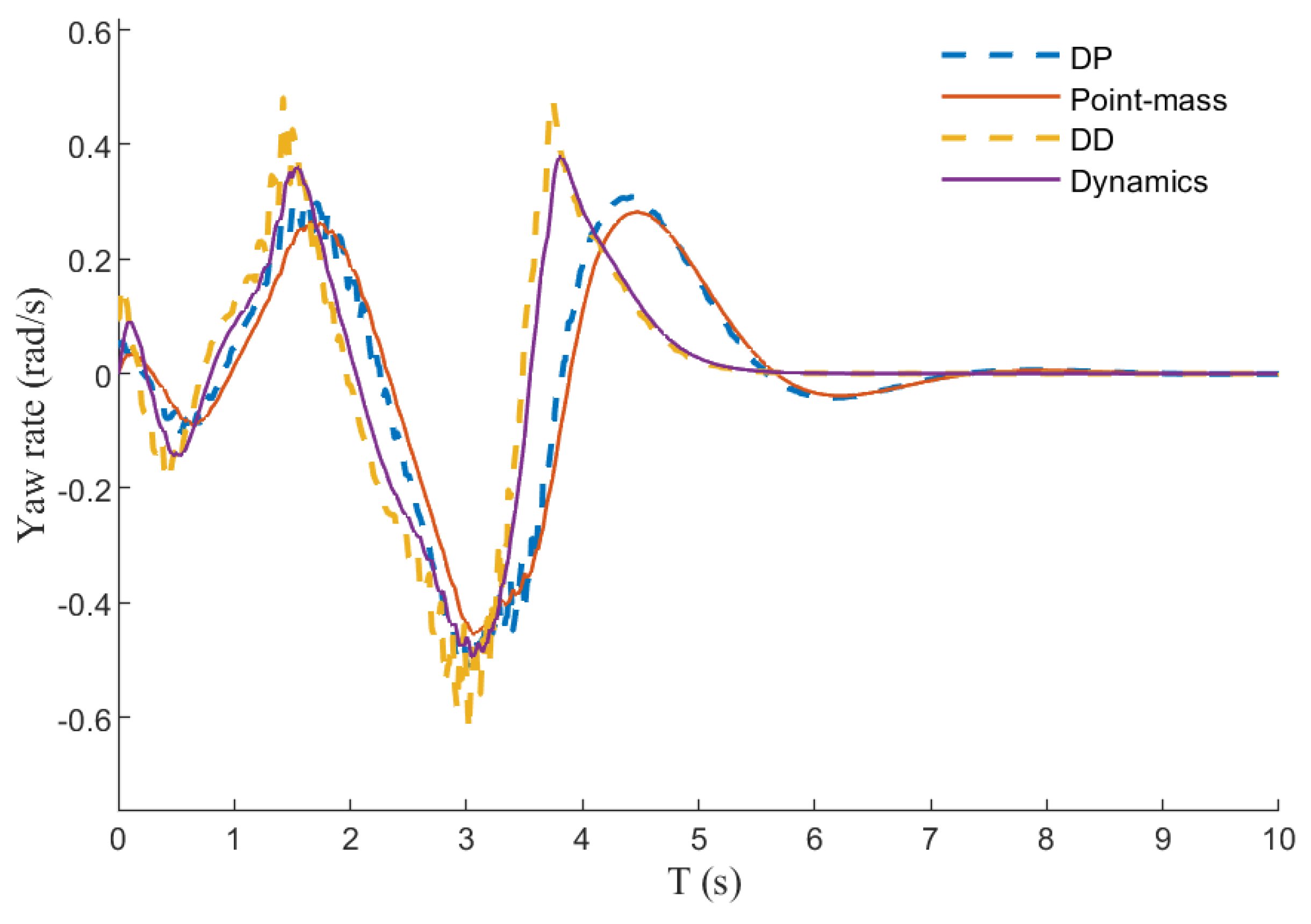
Figure 5 shows the yaw rate produced by the two planners at 20 m/s. “DP” represents the expected values of the comparative planner, and “DD” represents the expected values of the improved planner. It can be observed that the actual output yaw rate can effectively track the expected values. The output yaw rate of the improved planner exhibits a stable state. In comparison with the comparative planner, the output yaw rate slightly increases. This is due to the centrifugal force acting when the vehicle turns, causing the vehicle body to tilt towards the outside of the curve. The vertical load transfer generates a lateral yaw moment so considering this constraint results in a slight increase in the output yaw rate.

Figure 5. Comparison of yaw rate at 20 m/s.

Figure 5. Comparison of yaw rate at 20 m/s.

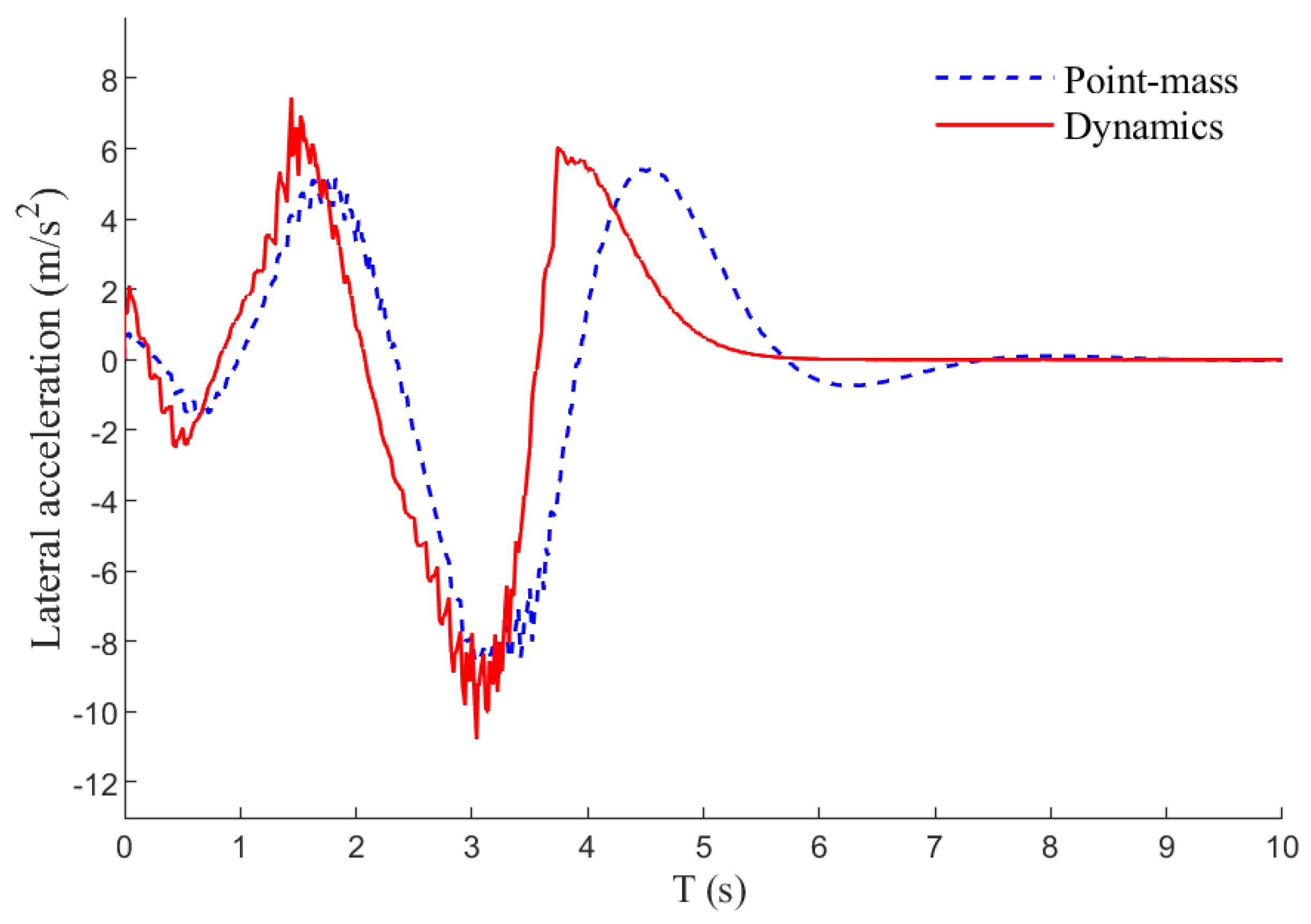
Figure 6 shows the lateral acceleration output at 20 m/s. The lateral acceleration of the improved planner is slightly greater than that of the comparative planner at each moment, and the curve trend is basically the same. This is because the improved planner can quickly complete the obstacle avoidance tracking behavior, resulting in larger steering angles.

Figure 6. Comparison of lateral acceleration at 20 m/s.

Figure 6. Comparison of lateral acceleration at 20 m/s.

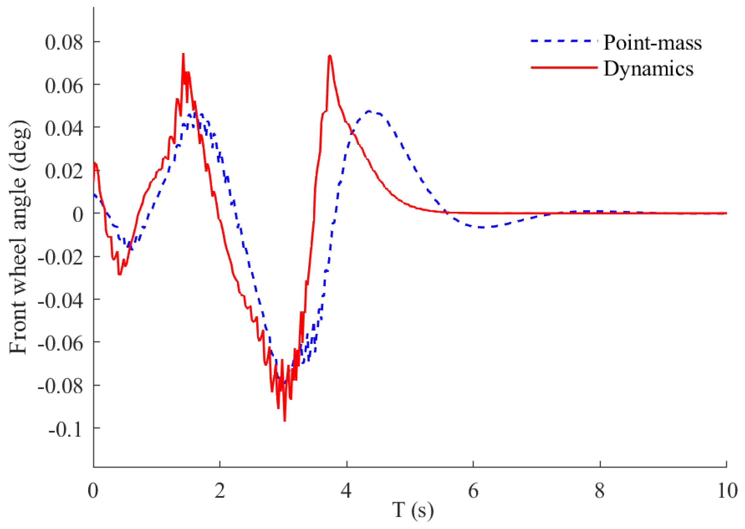
Figure 7 shows the front wheel steering angle output of the trajectory planner. It can be observed that the improved planner’s front wheel steering angle output is slightly higher than that of the comparative planner. The slightly higher front wheel steering angle indicates its more proactive steering measures during the vehicle’s motion, leading to better tracking of the planned trajectory. By increasing the front wheel steering angle when the lateral error is small, the vehicle can quickly adjust its heading, thereby reducing the accumulation of lateral error and enhancing the stability and precision of motion.

Figure 7. Comparison of front wheel steering angle at 20 m/s.

Figure 7. Comparison of front wheel steering angle at 20 m/s.

5.2. Simulation of 30 m/s

Setting the vehicle speed to 30 m/s, initial position to (0, 0), ground friction coefficient $m_u$ to 0.8, simulation time to 10 s, and time step to 0.02 s, the simulation results are as illustrated in Figure 8 and Figure 9.

Figure 8 shows the effects of trajectory planning and local obstacle avoidance planning at a speed of 30 m/s, while Figure 9 shows the lateral error of the planned trajectory. It can be observed that the improved planner has a maximum lateral error of 1.59 m during obstacle avoidance, significantly smaller than the maximum lateral error of 2.35 m for the comparative planner. The lateral error is reduced by 32.3%. Furthermore, after obstacle avoidance, the maximum lateral error of the improved planner in the first turn is 2.31 m, a reduction of 1.48 m compared to the comparative planner. This further illustrates the superior obstacle avoidance tracking performance of the improved planner. The lateral error of the improved planner approaches zero after X = 100 m, whereas the comparative planner achieves this after X = 170 m, indicating that the improved planner can quickly stabilize straight-line driving after high-speed cornering, and the lateral error exhibits better stability. From the above analysis, we conclude that the improved planner is significantly superior to the comparative planner in terms of obstacle avoidance effectiveness, high-speed cornering, and recovery ability, while ensuring overall planning and tracking accuracy.

Figure 9. Comparison of lateral error at 30 m/s.

Figure 9. Comparison of lateral error at 30 m/s.

Compared to 20 m/s, the increase in longitudinal speed leads to an increase in the distance between the planned trajectory and obstacles. However, the improved planner exhibits smaller lateral errors during obstacle avoidance, further highlighting its excellent nonlinear-constraint-based dynamic characteristics. Nevertheless, the lateral error between the planned trajectory and the reference trajectory increases during high-speed obstacle avoidance because the vehicle must balance vehicle stability and safety.

Additionally, the output of yaw rate, lateral acceleration, and front wheel steering angle at 30 m/s is similar to that at 20 m/s and is not discussed further. Ultimately, this verifies that considering the nonlinear constraints of vertical load transfer in trajectory planning results in superior dynamic characteristics.

6. Conclusions

This paper proposes a trajectory planning and tracking model predictive control method that considers vertical load variation factors using only a two-degrees-of-freedom vehicle dynamics model. Then, the solution problem of the constrained controller is transformed into a quadratic planning problem for the optimization. Simulink simulation results indicate that the improved planning controller in this study can generate an optimal collision-free path. Under the condition of a longitudinal speed of 20 m/s, compared to the trajectory planned by the reference planning controller, the lateral error is reduced by 53.5%, and the lateral error in local obstacle avoidance is reduced by 44.7%. Under the condition of 30 m/s, the lateral error is reduced by 32.3%, and the lateral error in local obstacle avoidance is reduced by 64.1%. Additionally, the robustness of the tracking system is validated by analyzing yaw rate, lateral acceleration, and front wheel steering angle at different speeds under the double-lane-change maneuver condition. As a result, the tracking controller can track the planned trajectory safely and smoothly. This method significantly improves the accuracy of trajectory planning and obstacle avoidance tracking, thereby enhancing the performance of autonomous vehicles. Future research will focus on validating this method through real vehicle experiments.

References

- Pan, R.; Jie, L.; Zhao, X.; Wang, H.; Yang, J.; Song, J. Active Obstacle Avoidance Trajectory Planning for Vehicles Based on Obstacle Potential Field and MPC in V2P Scenario. Sensors 2023, 23, 3248. [Google Scholar] [CrossRef]
- De Curtò, J.; de Zarzà, I.; Cano, J.C.; Manzoni, P.; Calafate, C.T. Adaptive Truck Platooning with Drones: A Decentralized Approach for Highway Monitoring. Electronics 2023, 12, 4913. [Google Scholar] [CrossRef]
- Zhao, C.; Zhu, Y.; Du, Y.; Liao, F.; Chan, C.Y. A Novel Direct Trajectory Planning Approach Based on Generative Adversarial Networks and Rapidly-Exploring Random Tree. IEEE Trans. Intell. Transp. Syst. 2022, 23, 17910–17921. [Google Scholar] [CrossRef]
- Vanhoek, R.; Ploeg, J.; Nijmeijer, H. Cooperative Driving of Automated Vehicles Using B-Splines For Trajectory Planning. IEEE Trans. Intell. Veh. 2021, 6, 594–604. [Google Scholar] [CrossRef]
- Tan, Z.; Wei, J.; Dai, N. Real-time dynamic trajectory planning for intelligent vehicles based on quintic polynomial. In Proceedings of the 2022 IEEE 21st International Conference on Ubiquitous Computing and Communications (IUCC/CIT/DSCI/SmartCNS), Chongqing, China, 19–21 December 2022; pp. 51–56. [Google Scholar]
- Shi, Y.; Chen, Y.; Jia, B. Local trajectory planning for autonomous trucks in collision avoidance maneuvers with rollover prevention. In Proceedings of the 2019 American Control Conference (ACC), Philadelphia, PA, USA, 10–12 July 2019; pp. 3981–3986. [Google Scholar]
- Rao, J.; Xiang, C.; Xi, J.; Chen, J.; Lei, J.; Giernacki, W.; Liu, M. Path planning for dual UAVs cooperative suspension transport based on artificial potential field-A* algorithm. Knowl.-Based Syst. 2023, 277, 110797. [Google Scholar] [CrossRef]
- Zhang, W.; Wang, N.; Wu, W. A hybrid path planning algorithm considering AUV dynamic constraints based on improved A* algorithm and APF algorithm. Ocean. Eng. 2023, 285, 115333. [Google Scholar] [CrossRef]
- Jiang, Z.; Zhang, X.; Wang, P. Grid-Map-Based Path Planning and Task Assignment for Multi-Type AGVs in a Distribution Warehouse. Mathematics 2023, 11, 2802. [Google Scholar] [CrossRef]
- Wu, D.M.; Li, Y.; Du, C.Q.; Ding, H.T.; Li, Y.; Yang, X.B.; Lu, X.Y. Fast Velocity Trajectory Planning and Control Algorithm of Intelligent 4WD Electric Vehicle for Energy Saving Using Time-Based MPC. IET Intell. Transp. Syst. 2019, 13, 153–159. [Google Scholar] [CrossRef]
- Zuo, Z.; Yang, X.; Li, Z.; Wang, Y.; Han, Q.; Wang, L.; Luo, X. MPC-Based Cooperative Control Strategy of Path Planning and Trajectory Tracking for Intelligent Vehicles. IEEE Trans. Intell. Veh. 2021, 6, 513–522. [Google Scholar] [CrossRef]
- Jones, M.; Djahel, S.; Welsh, K. Path-planning for unmanned aerial vehicles with environment complexity considerations: A survey. ACM Comput. Surv. 2023, 55, 1–39. [Google Scholar] [CrossRef]
- Rowold, M.; Ögretmen, L.; Kasolowsky, U.; Lohmann, B. Online time-optimal trajectory planning on three-dimensional race tracks. In Proceedings of the 2023 IEEE Intelligent Vehicles Symposium (IV), Anchorage, AK, USA, 4–7 June 2023; pp. 1–8. [Google Scholar]
- Chen, X.; Liu, S.; Zhao, J.; Wu, H.; Xian, J.; Montewka, J. Autonomous port management based AGV path planning and optimization via an ensemble reinforcement learning framework. Ocean. Coast. Manag. 2024, 251, 107087. [Google Scholar] [CrossRef]
- Victor, S.; Receveur, J.B.; Melchior, P.; Lanusse, P. Optimal Trajectory Planning and Robust Tracking Using Vehicle Model Inversion. IEEE Trans. Intell. Transp. Syst. 2022, 23, 4556–4569. [Google Scholar] [CrossRef]
- Yang, B.; Zhang, H.; Jiang, Z. Path planning and tracking control for automatic driving obstacle avoidance. In Proceedings of the 2019 International Conference on Robotics, Intelligent Control and Artificial Intelligence (RICAI 2019), Shanghai, China, 20–22 September 2019; pp. 300–304. [Google Scholar]
- Yin, Y.; Rakheja, S.; Boileau, P.-E. A Roll Stability Performance Measure for Off-Road Vehicles. J. Terramech. 2016, 64, 58–68. [Google Scholar] [CrossRef]
- Wang, J.; Yan, Y.; Zhang, K.; Chen, Y.; Cao, M.; Yin, G. Path Planning on Large Curvature Roads Using Driver-Vehicle-Road System Based on the Kinematic Vehicle Model. IEEE Trans. Veh. Technol. 2022, 71, 311–325. [Google Scholar] [CrossRef]
- Tahirovic, A.; Magnani, G. Passivity-based model predictive control for mobile robot navigation planning in rough terrains. In Proceedings of the IEEE/RSJ 2010 International Conference on Intelligent Robots And Systems (IROS 2010), Taipei, Taiwan, 18–22 October 2010; pp. 307–312. [Google Scholar]
- Liu, Q.; Song, S.; Hu, H.; Huang, T.; Li, C.; Zhu, Q. Extended Model Predictive Control Scheme for Smooth Path Following of Autonomous Vehicles. Front. Mech. Eng. 2022, 17, 4. [Google Scholar] [CrossRef]
- Kanchwala, H. Path planning and tracking of an autonomous car with high fidelity vehicle dynamics model and human driver trajectories. In Proceedings of the 2019 IEEE 10th International Conference on Mechanical and Aerospace Engineering (ICMAE 2019), Brussels, Belgium, 22–25 July 2019; pp. 306–313. [Google Scholar]
- Li, B.; Zhang, B.; Du, H.; Wu, Y.; Chen, S. Trajectory Planning, Dynamics Modelling and Trajectory Tracking Method for Off-Road Autonomous Vehicles Considering the Road Topography Information. Int. J. Veh. Des. 2021, 87, 170–198. [Google Scholar] [CrossRef]
- Kanchwala, H.; Bezerra Viana, I.; Aouf, N. Cooperative Path-Planning and Tracking Controller Evaluation Using Vehicle Models of Varying Complexities. Proc. Inst. Mech. Eng. Part C J. Mech. Eng. Sci. 2021, 235, 2877–2896. [Google Scholar] [CrossRef]
- Yao, J.; Lv, G.; Qv, M.; Li, Z.; Ren, S.; Taheri, S. Lateral Stability Control Based on the Roll Moment Distribution Using a Semiactive Suspension. Proc. Inst. Mech. Eng. Part D J. Automob. Eng. 2016, 231, 1627–1639. [Google Scholar] [CrossRef]
- Yao, J.; Wang, M.; Li, Z.; Jia, Y. Research on Model Predictive Control for Automobile Active Tilt Based on Active Suspension. Energies 2021, 14, 671. [Google Scholar] [CrossRef]
- Falcone, P.; Eric Tseng, H.; Borrelli, F.; Asgari, J.; Hrovat, D. MPC-Based Yaw and Lateral Stabilisation via Active Front Steering and Braking. Veh. Syst. Dyn. 2008, 46, 611–628. [Google Scholar] [CrossRef]
- Yao, J.; Wang, M.; Bai, Y. Automobile Active Tilt Based on Active Suspension with H∞ Robust Control. Proc. Inst. Mech. Eng. Part D J. Automob. Eng. 2020, 235, 1320–1329. [Google Scholar] [CrossRef]