Predefined-Time Tracking Control of Unmanned Surface Vehicle under Complex Time-Varying Disturbances

Abstract

Aiming at the unmanned surface vehicle (USV) trajectory tracking control under complex time-varying environment, a predefined-time convergence sliding mode disturbance observer (PTC-SMO) is introduced to effectively handle the internal parameter uncertainties and external environmental disturbances, thereby guaranteeing precise compensation of the lumped disturbance term within a set time. Then, in order to achieve precise tracking of the desired trajectory using USV under a predetermined time constraint, a novel fast trajectory tracking control strategy with predefined-time convergence (PTC-FTTCS) is established to improve tracking performance and ensure that the trajectory tracking error converges quickly in the predefined time. Through rigorous comparative simulation under ideal conditions and time-varying disturbances, the results demonstrate reliable trajectory tracking and disturbance handling effects, and the tracking performance and disturbance observation performance are significantly better than state-of-the-art methods.

1. Introduction

Unmanned Surface Vehicles (USVs) represent a groundbreaking advancement in maritime technology, offering highly intelligent decision-making capabilities without the need for manual intervention [1,2]. These cutting-edge platforms are transforming a wide range of maritime operations, from resource surveying to military endeavors. Amidst the rapid progression of unmanned technologies, the field of intelligent motion control has attracted significant attention. However, the dynamic nature of the USV system, characterized by strong time variability, intricate coupling, and considerable uncertainty, poses substantial challenges. These systems are subjected to complex disturbances, including external winds, waves, and ocean currents, complicating the development of precise system motion models and the achievement of accurate trajectory tracking [3].

Trajectory tracking control, fundamental to the operational efficacy of USV, refers to controlling the USV to steadily move along the desired trajectory in global time. In order to achieve precise trajectory tracking, prevalent control methodologies encompass include adaptive control [4,5,6], fuzzy control [7,8], model predictive control [9], neural network control [6,10,11] and sliding mode control [12,13]. Among these, sliding mode control is distinguished for its robustness, simplicity, and low sensitivity to parameter variations and external disturbances, rendering it highly effective for USV controller design [14]. Chen [15] introduced an adaptive sliding mode control algorithm to enhance the stabilization of the heading angle and reduce longitudinal speed tracking errors, achieving robust global asymptotic stability, but the impact of chattering near the sliding surface is relatively large; Wang [16] proposed a novel non-singular terminal sliding mode approach law, incorporating variable exponential reaching laws for the trajectory tracking control, thereby enhancing the convergence rate and reducing the chattering phenomenon. Nonetheless, these strategies did not adequately address the impact on the tracking system’s convergence time; Fan [17] proposed a finite-time back-stepping control strategy that ensures system convergence to a near-zero bounded region within a finite-time, Nonetheless, these strategies did not adequately address the impact on the tracking system’s convergence time. This method’s effectiveness, however, is highly dependent on the system’s initial conditions. To mitigate the issue, Ghommam [18] introduced an adaptive neural network-based fixed-time control strategy, ensuring the tracking error of the USV converges to zero within a fixed time.

It is crucial to highlight that within the sphere of practical engineering implementations, the necessity for predefining both convergence time and tracking accuracy is paramount. Introducing an excessive number of control parameters can, paradoxically, detract from controller performance. The concept of predefined time stability, which dictates the maximum allowable system convergence time to meet specific task demands, has recently gained traction in control method research. Juan [19] proposed a novel sliding mode control method with predefined-time convergence and authenticated the ability of the system to reach an equilibrium state within the stipulated convergence time. Becerra [20] introduced a motor control strategy predicated on predefined-time stability and corroborated its effectiveness through empirical trials. Yang [21] investigated the predefined-time formation tracking problem of networked NASVs under external disturbances and proposed a hierarchical time-triggered control scheme with predefined-time stability. The estimator reduces the frequency of control signal updates and communication overhead. Liang [22] designed a class of hierarchical control algorithms based on the newly proposed predefined-time sliding mode surface to address the formation tracking control problem of NMSVs under various conditions. Liang [23] introduced a predefined-time optimization control strategy subjected to set constraints, wherein a distributed optimization estimator calculates the optimal solutions under geometric constraints. Additionally, a singularity avoidance scheme was devised to tackle issues related to system singularities. Based on the excellent control performance of predefined time control, this paper attempts to design an efficient USV trajectory tracking controller by combining predefined time control theory and sliding mode control.

Moreover, the trajectory tracking control accuracy of USVs is significantly impacted by intricate internal and external elements such as wind, waves, system actuator malfunctions, and unmodeled dynamics. In ideal navigation conditions without the aforementioned complex disturbances, tracking controllers designed based on sliding mode control can basically achieve reliable expected trajectory tracking. However, as the complexity of the disturbance increases, the control effect is greatly reduced. In [10], a finite time disturbance observer was designed to achieve precise observation and compensation of disturbances for trajectory tracking control of USV under constant external disturbances. Qu [14] further improves the sliding mode control structure to enhance anti-interference performance and achieve continuous observation of disturbances. In addition, in practical environments, external disturbances are unpredictable and time-varying, posing a huge challenge to the accuracy of trajectory tracking control. To eliminate the lumped disturbance interference, Li [24] focused on the unmodeled dynamics and input saturation of the USV system, devising a filtered extended state observer to efficaciously monitor complex interferences and improve model robustness. Wu [25] developed a terminal sliding mode observer with limited input saturation, ensuring swift convergence of observation errors in the face of unknown velocities and adeptly handling inputs under uncertain constraints. Li [26] treated external disturbances as the lumped disturbance terms, introducing a disturbance observer characterized by fixed-time stable convergence, with convergence time independent of initial conditions. Inspired by the predefined-time control theory and disturbance observer technology, this paper proposes a novel disturbance observer with predefined-time convergence to achieve accurate observation of lumped disturbance terms.

To summarize, the domain of intelligent control for USV is significantly enriched by the potential applications of predefined-time control theory. Utilizing the foundational principles of sliding mode control, alongside the technologies of disturbance observer and predefined-time stability theory, this paper proposes an efficient tracking control strategy and an accurate disturbances observer. The main contributions of this paper include:

(1) For trajectory tracking control of USV under the ideal state, a novel fast integral terminal sliding mode tracking strategy is proposed by combining integral sliding mode and terminal sliding mode to keep the USV continuously and stably navigating along the set trajectory without disturbance.

(2) For complex disturbance environments, a novel fast trajectory tracking control strategy with predefined-time convergence (PTC-FTTCS). This strategy enables the USV to move along a planned trajectory in dynamic and uncertain environments and ensure that the tracking error converges within a predefined time, which improves reliable control performance in engineering applications.

(3) To mitigate the impact of external complex disturbances and unreliable model parameters, a sliding mode disturbance observe with predefined-time convergence (PTC-SMO) is improved to for observing and approximating internal unknown parameter perturbations and time-varying complex disturbances, improving system stability and robustness. The proposed tracking controller and disturbance observer are further corroborated by thorough comparative simulation experiments.

The rest of this paper is organized as follows: Section 2 focuses on explaining the mathematical model of USV and lemmas, as well as the design process of the USV tracking controller under ideal conditions. Section 3 provides a detailed introduction to the design process of disturbance observer and predefined time tracking controller. Section 4 provides a rigorous discussion of simulation experiments. Section 5 provides the conclusion and outlook of the entire paper.

2. Theoretical Basis and System Model

2.1. Basic Theories of Predefined-Time Convergence

Refer to the following system model:

$$\begin{array}{c}\hfill \begin{array}{c}\dot{x}\left(t\right)=f\left(x\left(t\right)\right)\hfill \\ x\left(0\right)={\mathrm{x}}_0,f\left(0\right)=0,x\in U_0\subset R^n\hfill \end{array}\end{array}$$

(1)

where x is the variable of system and $f\left(x\right(t\left)\right)$ is delineated as a continuous nonlinear function within the vicinity of the origin $U_0$.

Definition 1 

([27]). If system (1) exhibits negative homogeneity coupled with asymptotic stability, enabling it to reach its equilibrium state within a finite time $T_p$, then system (1) is characterized as globally finite-time stable. It is worth mentioning that this finite time $T_p$ is contingent upon the initial configuration of the system.

Definition 2 

([28]). In the event that system (1) achieves global finite-time stability, with the convergence time $T_p$ possessing a supreme limit that does not depend on the initial state of the system, such a system is then defined as globally fixed-time stable.

Definition 3 

([19]). Further assuming that system (1) qualifies as a globally fixed-time stable system, and the state convergence time $T_p$ is subject to a minimal supreme limit that is precisely incorporated in the function, then the system is a globally predefined time stable system, this configuration elevates the system to be globally predefined-time stable.

Lemma 1 

([29]). Consider the system as shown below:

$$\begin{array}{c}\hfill \dot{x}=-\frac{h(+\infty )-h\left(0\right)}{T_c}{\left[\frac{\partial h\left(x^m\right)}{\partial x}\right]}^{-1}\end{array}$$

(2)

where $0<m<1$, $T_c>0$. If the bounded function satisfies the following conditions:

(1) $h\left(x\right)$ is continuous within the range of $(0,+\infty )$ and satisfies $h\left(0\right)=0$;

(2) $\underset{\delta \to 0}{lim}\frac{h({\left|x\right|}^m+\delta )-h\left({\left|x\right|}^m\right)}{\delta }>0$;

(3) $\underset{x\to 0}{lim}{\left[\frac{\partial h\left(x^m\right)}{\partial x}\right]}^{-1}=0,{\left[\frac{\partial h\left(x^m\right)}{\partial x}\right]}^{-1}{\mid }_{x=0}=0$;

then the system converges at a predefined time with the convergence time $T<T_c$.

Lemma 2 

([30]). For a Lyapunov function $V\left(x\right)$ with globally positive definite, if the derivative satisfies:

$$\begin{array}{c}\hfill \dot{V}\le -\frac{h(+\infty )-h\left(0\right)}{T_s}{\left[\frac{\partial h\left(V^m\right)}{\partial V}\right]}^{-1}+c\end{array}$$

(3)

where the definition of $h\left(V^m\right)$ is consistent with Lemma 1, and c is a constant, $0<m<1$, $T_c>0$. Then the system state x will converge to a small area near the origin within the predefined time $T_c$. Subsequently, the state of the system x is guaranteed to approach a vicinity in close proximity to the origin, achieving this convergence within a predefined time $T_c$. In actual control systems, due to factors such as modeling errors and sampling delays, it is impossible to achieve predefined time control that accurately converges to the origin and can only achieve actual predefined time convergence to a small neighborhood near the origin.

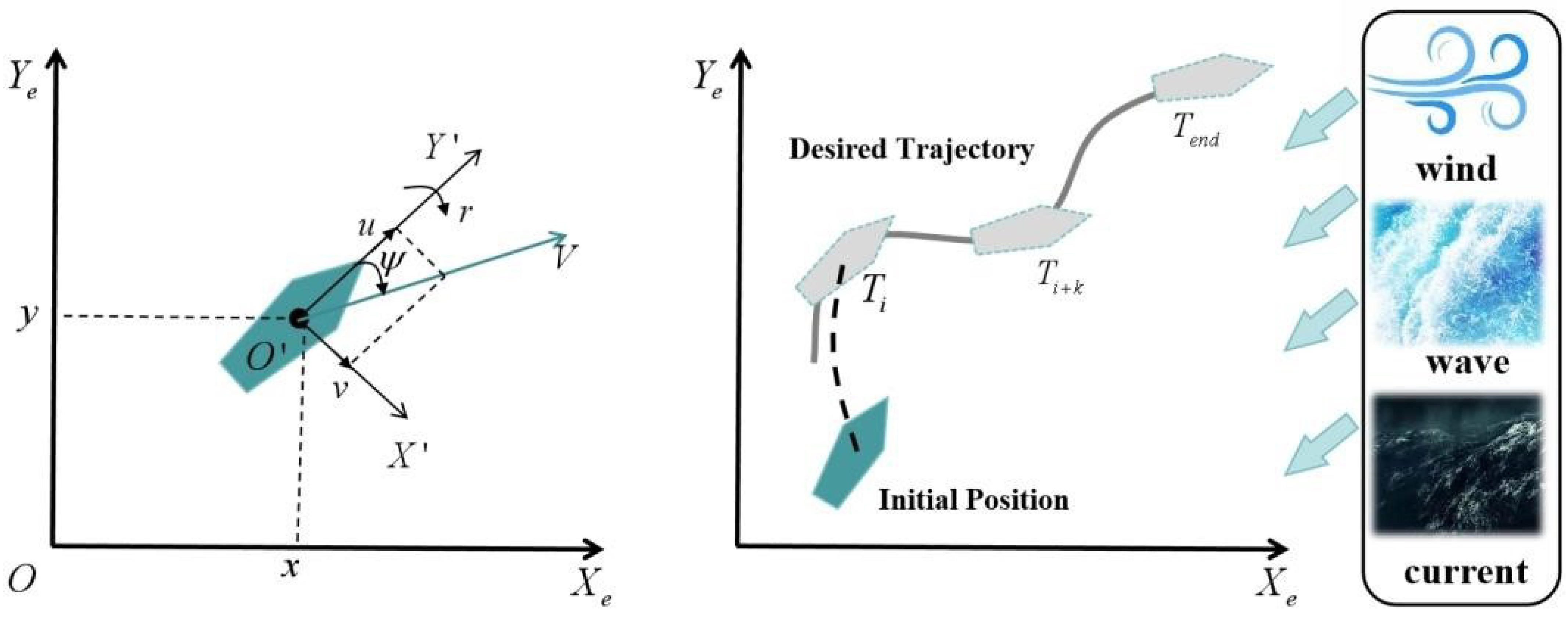
2.2. USV Mathematical Model

The USV has the characteristics of strong coupling, strong nonlinearity, and high complexity in actual maritime navigation. Therefore, unmodeled dynamics and various external disturbances cannot be ignored when establishing a USV model, and an overly simple USV model lacks practicality and generality, but an overly complicated model will handle subsequent controller design impossible. Hence, when establishing the UAV model, we cannot consider the ideal state and ignore the uncertainty terms composed of hydrodynamic derivatives within the system, as well as the external complex disturbances composed of strong winds, waves, and undercurrents, which makes it difficult to work on the bottom execution mechanism and cannot fully control the six degree-of-freedom USV model. In this paper, the three degree-of-freedom model is considered to solve the USV tracking problem, which revolves around establishing the relationship between surging speed u, swaying speed v, and yawing angular speed r, and ignores the heave speed, roll angular speed, and pitch angular speed.

As shown in Figure 1, it can be seen that the dynamics and kinematics equations of the USV are as follows:

$$\begin{array}{c}\hfill \left\{\begin{array}{c}\dot{\mathit{\eta }}=\mathit{R}\left(\mathit{\psi }\right)\mathit{\nu }\hfill \\ \mathit{M}\dot{\mathit{\nu }}+\mathit{C}\left(\mathit{\nu }\right)\mathit{\nu }+\mathit{D}\left(\mathit{\nu }\right)\mathit{\nu }=\mathit{\tau }+\mathit{\delta }\hfill \end{array}\right.\end{array}$$

(4)

where $\mathit{\eta }={[x,y,\psi ]}^{\mathrm{T}}$ represents the position vector of the USV, $\mathit{\nu }={[u,v,r]}^{\mathrm{T}}$ signifies the velocity vector, $\psi$ is defined as the heading angle, and r is the angular velocity. The control input vector, $\mathit{\tau }={[{\tau }_{\mathrm{i}1},0,{\tau }_{\mathrm{i}3}]}^{\mathrm{T}}$, comprises the thrust moment ${\tau }_{i1}$ in the surge direction and the yaw moment ${\tau }_{i3}$, reflecting the directional control efforts. The term $\mathit{\delta }=M{R}^{\mathrm{T}}\left(\psi \right)d\left(t\right)$, $d\left(t\right)$ represents the vector of complex disturbances emanating from environmental forces such as wind, waves, and ocean currents. The inertia matrix $\mathit{M}={\mathit{M}}^{\mathrm{T}}>0$ is symmetric and positive definite, which integrates the rigid body’s inertia matrix with that of the added mass. The Coriolis matrix $\mathit{C}\left(\mathit{\nu }\right)=-\mathit{C}{\left(\mathit{\nu }\right)}^{\mathrm{T}}$ is skew-symmetric with its parameters derived from multiple hydrodynamic coefficients obtained through sea trials. Additionally, $\mathit{D}\left(\mathit{\nu }\right)$ describes the damping matrix that accounts for both linear and nonlinear resistance forces acting on the hull. These matrices are characterized as follows:

$$\begin{array}{c}\hfill \mathit{M}=\left[\begin{array}{ccc}{m}_{11}& 0& 0\\ 0& m_{22}& m_{23}\\ 0& m_{32}& m_{33}\end{array}\right]\end{array}$$

(5)

$$\begin{array}{c}\hfill \mathit{C}\left(\mathit{\nu }\right)=\left[\begin{array}{ccc}0& 0& c_{13}\left(\nu \right)\\ 0& 0& c_{23}\left(\nu \right)\\ -c_{13}\left(\nu \right)& -c_{23}\left(\nu \right)& 0\end{array}\right]\end{array}$$

(6)

$$\begin{array}{c}\hfill \mathit{D}\left(\mathit{v}\right)=\left[\begin{array}{ccc}{d}_{11}\left(\nu \right)& 0& 0\\ 0& d_{22}\left(\nu \right)& d_{23}\left(\nu \right)\\ 0& -d_{32}\left(\nu \right)& d_{33}\left(\nu \right)\end{array}\right]\end{array}$$

(7)

Matrix parameters are delineated in

Table 1. The matrix parameters definition.

Parameters	Values	Parameters	Values
$m_{11}$	${m-X}_{\dot{\mu }}$	$c_{23}\left(v\right)$	$m_{11}\mu$
$m_{22}$	${m-Y}_{\dot{v}}$	$d_{11}\left(v\right)$	$-X_{\mu }-X_{\left|\mu \right|\mu }\left|\mu \right|$
$m_{23}$	${m{x}_g-Y}_{\dot{r}}$	$d_{22}\left(v\right)$	$-X_u-X_{\left|u\right|u}\left|u\right|-X_{uuu}{u}^2$
$m_{32}$	${m{x}_g-N}_{\dot{v}}$	$d_{23}\left(v\right)$	$-Y_r-Y_{\left|v\right|r}\left|v\right|-Y_{\left|r\right|r}\left|r\right|$
$m_{33}$	${I_z-N}_{\dot{r}}$	$d_{32}\left(v\right)$	$-N_v-N_{\left|v\right|v}\left|v\right|-N_{\left|r\right|v}\left|r\right|$
$c_{13}\left(v\right)$	$-m_{11}-m_{23}r$	$d_{33}\left(v\right)$	$-N_r-N_{\left|v\right|r}\left|v\right|-N_{\left|r\right|r}\left|r\right|$

, where m signifies the mass, L denotes the length, B represents the width of, and $x_g$ represents the center of gravity along the X axis within the body-fixed coordinate system. $I_z$ represents the moment of inertia and $N_{\dot{v}}=Y_{\dot{r}},X_{\ast },Y_{\ast },Z_{\ast }$ represents the hydrodynamic derivative of the USV.

The $\mathit{R}$ is the transformation matrix bridging the inertial and body-fixed coordinate systems:

$$\begin{array}{c}\hfill \mathit{R}\left(\mathit{\psi }\right)=\left[\begin{array}{ccc}cos\psi & -sin\psi & 0\\ sin\psi & cos\psi & 0\\ 0& 0& 1\end{array}\right]\end{array}$$

(8)

The matrix $\mathit{R}$ also has the following properties:

$$\begin{array}{c}\hfill \begin{array}{c}\dot{\mathit{R}}\left(\mathit{\psi }\right)=\mathit{R}\left(\mathit{\psi }\right)\mathit{S}\left(r\right)\hfill \\ {\mathit{R}}^{\mathrm{T}}\left(\mathit{\psi }\right)\mathit{S}\left(r\right)\mathit{R}\left(\mathit{\psi }\right)=\mathit{R}\left(\mathit{\psi }\right)\mathit{S}\left(r\right){\mathit{R}}^{\mathrm{T}}\left(\mathit{\psi }\right)=\mathit{S}\left(r\right)\hfill \\ ∥\mathit{R}\left(\mathit{\psi }\right)∥=1,{\mathit{R}}^{\mathrm{T}}\left(\mathit{\psi }\right)\mathit{R}\left(\mathit{\psi }\right)=\mathrm{I},\forall \mathit{\psi }\in [0,2\pi ]\hfill \end{array}\end{array}$$

(9)

Define expected tracking trajectory:

$$\begin{array}{c}\hfill \left\{\begin{array}{c}\dot{{\mathit{\eta }}_d}=\mathit{R}\left({\mathit{\psi }}_{\mathit{d}}\right){\mathit{\nu }}_{\mathit{d}}\hfill \\ {\mathit{M}}_{\mathit{d}}{\dot{\mathit{\nu }}}_{\mathit{d}}+\mathit{C}\left({\mathit{\nu }}_{\mathit{d}}\right){\mathit{\nu }}_{\mathit{d}}+\mathit{D}\left({\mathit{\nu }}_{\mathit{d}}\right){\mathit{\nu }}_{\mathit{d}}={\mathit{\tau }}_{\mathit{d}}\hfill \end{array}\right.\end{array}$$

(10)

where ${\mathit{\tau }}_{\mathit{d}}={[{\tau }_{d1},0,{\tau }_{d3}]}^{\mathrm{T}}$ indicates the desired control input of the USV, while ${\mathit{\eta }}_{\mathit{d}}={[{\mathrm{x}}_d,{\mathrm{y}}_d,{\psi }_d]}^{\mathrm{T}}$ and ${\mathit{\nu }}_{\mathit{d}}={[{\mathrm{u}}_d,{\mathrm{v}}_d,r_d]}^{\mathrm{T}}$, respectively, represent the position and velocity vector of expected tracking trajectory.

2.3. Design of USV Tracking Controller under Ideal Conditions

In this section, this paper initially concentrates on the USV trajectory tracking control under ideal conditions. Specifically, a USV tracking control strategy based on the fast integral terminal sliding mode (FITSMC) is proposed, integrating both integral sliding mode and terminal sliding mode to significantly enhance tracking effectiveness.

From Formula (4), we can obtain:

$$\begin{array}{c}\hfill \ddot{\mathit{\eta }}=\mathit{R}{\mathit{M}}^{-1}\mathit{\tau }-\mathit{R}{\mathit{M}}^{-1}\mathrm{A}\left(\mathit{\eta },{\mathit{R}}^T\mathit{\nu }\right)\dot{\mathit{\eta }}+\mathit{S}\dot{\mathit{\eta }}\end{array}$$

(11)

where

$$\begin{array}{c}\hfill \mathrm{A}\left(\mathit{\eta },{\mathit{R}}^T\mathit{\nu }\right)=\left(\mathit{C}\left(\mathit{\nu }\right)+\mathit{D}\left(\mathit{\nu }\right)\right){\mathit{R}}^T\end{array}$$

(12)

The position error between the actual and desired positions is described as follows:

$$\begin{array}{c}\hfill \mathit{e}=\mathit{\eta }-{\mathit{\eta }}_{\mathit{d}}\end{array}$$

(13)

The FITSMS is designed as follows:

$$\begin{array}{c}\hfill \mathit{s}=\mathit{e}+{\lambda }_1\int \mathit{e}d\tau +{\lambda }_2\int {\mathit{e}}^{q/\phantom{qp}p}d\tau \end{array}$$

(14)

The derivation of the s satisfies:

$$\begin{array}{c}\hfill \dot{\mathit{s}}=\ddot{\mathit{e}}+{\lambda }_1\mathit{e}+{\lambda }_2{\mathit{e}}^{q/\phantom{qp}p}\end{array}$$

(15)

To enhance the approach velocity towards the sliding mode surface while maintaining stability during the sliding phase, a novel approach law is instituted as:

$$\begin{array}{c}\begin{array}{c}\dot{\mathit{s}}=-\epsilon {\left[{\mathit{s}}^2+f\left(\mathit{e}\right){\dot{\mathit{e}}}^2\right]}^{\raisebox{1ex}{$\alpha $}\!\left/ \!\raisebox{-1ex}{$2$}\right.}\mathit{sgn}\left(s\right)-k{\left|\mathit{e}\right|}^{\beta }s\hfill \end{array}\hfill \\ f\left(\mathit{e}\right)=\{\begin{array}{cc}\xi {\left({\Delta }_2/\phantom{{\Delta }_2\left|\mathit{e}\right|}\left|\mathit{e}\right|\right)}^2& \left|\mathit{e}\right|>{\Delta }_2\\ \xi & {\Delta }_1<\left|\mathit{e}\right|\le {\Delta }_2\\ \xi {\left(\left|\mathit{e}\right|/\phantom{\left|\mathit{e}\right|{\Delta }_1}{\Delta }_1\right)}^2& \left|\mathit{e}\right|\le {\Delta }_1\end{array}\end{array}$$

(16)

among them, $\epsilon$, $\alpha$, $\beta$, k, ${\Delta }_1$, ${\Delta }_2$, $\xi$ are all positive constants and satisfy ${\Delta }_1>{\Delta }_2$, where $k{\left|e\right|}^{\beta }s$ indicates the fast approach term, and $\epsilon {\left[s^2+f\left(e\right){\dot{e}}^2\right]}^{\raisebox{1ex}{$\alpha $}\!\left/ \!\raisebox{-1ex}{$2$}\right.}$sgn(s) indicates the variable speed approach component. If the discrepancy e is too large or too small, the variable speed approach term will adjust the rate of approaching the sliding mode surface to avoid sharp changes in output due to large changes in speed or normal fluctuations.

Then, the FITSMC trajectory tracking control strategy is designed as follows:

$$\begin{array}{cc}\mathit{\tau }=\hfill & \mathrm{A}\left(\mathit{\eta },{\mathit{R}}^T\mathit{\nu }\right)\dot{\mathit{\eta }}-\mathit{M}{\mathit{R}}^{-1}\mathit{\epsilon }{\left[{\mathit{s}}^2+f\left(\mathit{e}\right){\dot{\mathit{e}}}^2\right]}^{\raisebox{1ex}{$\alpha $}\!\left/ \!\raisebox{-1ex}{$2$}\right.}-\mathit{M}{\mathit{R}}^{-1}k{\left|\mathit{e}\right|}^{\beta }s\hfill \\ & -\mathit{M}{\mathit{R}}^{-1}\mathit{S}\dot{\eta }+\mathit{M}{\mathit{R}}^{-1}{\ddot{\mathit{\eta }}}_d-\mathit{M}{\mathit{R}}^{-1}({\lambda }_1\mathit{e}+{\lambda }_2{\mathit{e}}^{q/p})\hfill \end{array}$$

(17)

To substantiate the stability of the aforementioned tracking controller, a Lyapunov function is employed for the stability verification as follows:

$$\begin{array}{c}\hfill \mathit{V}=\frac{1}{2}{\mathit{s}}^2\end{array}$$

(18)

Taking the derivative of (18):

$$\begin{array}{c}\hfill \begin{array}{cc}\hfill \dot{\mathit{V}}=& \mathit{s}\dot{\mathit{s}}\hfill \\ \hfill =& \mathit{s}\left(\ddot{\mathit{e}}+{\lambda }_1\mathit{e}+{\lambda }_2{\mathit{e}}^{q/\phantom{qp}p}\right)\hfill \\ \hfill =& \mathit{s}\left(\ddot{\mathit{\eta }}-{\ddot{\mathit{\eta }}}_r+{\lambda }_1\mathit{e}+{\lambda }_2{\mathit{e}}^{q/\phantom{qp}p}\right)\hfill \\ \hfill =& \mathit{s}\left(\mathit{R}{\mathit{M}}^{-1}\mathit{\tau }-\mathit{R}{\mathit{M}}^{-1}\mathrm{A}\left(\mathit{\eta },{\mathit{R}}^T\mathit{\nu }\right)\dot{\mathit{\eta }}+\mathit{S}\dot{\mathit{\eta }}-{\ddot{\mathit{\eta }}}_r+{\lambda }_1\mathit{e}+{\lambda }_2{\mathit{e}}^{q/\phantom{qp}p}\right)\hfill \\ \hfill =& \mathit{s}\left(-\epsilon {\left[{\mathit{s}}^2+f\left(\mathit{e}\right){\dot{\mathit{e}}}^2\right]}^{\raisebox{1ex}{$\alpha $}\!\left/ \!\raisebox{-1ex}{$2$}\right.}\right.sgn\left(\mathit{s}\right)-k{\left|\mathit{e}\right|}^{\beta }\mathit{s})\hfill \\ \hfill =& -\epsilon {\left[{\mathit{s}}^2+f\left(\mathit{e}\right){\dot{\mathit{e}}}^2\right]}^{\raisebox{1ex}{$\alpha $}\!\left/ \!\raisebox{-1ex}{$2$}\right.}\mathit{s}-k{\left|\mathit{e}\right|}^{\beta }{\mathit{s}}^2<0\hfill \end{array}\end{array}$$

(19)

Combining Definition 1, the designed FITSMC tracking control strategy can converge within a finite time, thereby ensuring prompt and steady adherence to the envisaged trajectory under optimal conditions.

3. Design of Tracking Controller for USV under Complex Disturbances

In actual marine navigation environments, due to the limitations of experimental environments, the fluid dynamics and other parameters inside USV cannot be fully obtained. Moreover, the interference of wind, waves, and currents during the USV navigation process also brings significant challenges to the tracking control accuracy. This section combines predefined time control theory, sliding mode control, and disturbance observer technology to design a predefined time disturbance observer and accurate trajectory tracking controller.

3.1. Predefined Time Disturbance Observer

In order to simplify the subsequent analysis, Equation (4) is updated as follows:

$$\begin{array}{c}\hfill \left\{\begin{array}{c}{\dot{\mathit{x}}}_1={\mathit{x}}_2\hfill \\ {\dot{\mathit{x}}}_2={\mathit{M}}^{-1}\left({\mathit{x}}_1\right)\mathit{R}\left({\mathit{x}}_1\right)\mathit{\tau }+\mathsf{\Theta }\hfill \end{array}\right.\end{array}$$

(20)

where ${\mathit{x}}_1=\mathit{\eta }$, ${\mathit{x}}_2=\dot{\mathit{\eta }}$, the parameter $\mathsf{\Theta }={\mathit{M}}^{-1}\left[\mathit{\delta }\left(t\right)-\mathit{C}({\mathit{x}}_1,{\mathit{x}}_2){\mathit{x}}_2-\mathit{D}({\mathit{x}}_1,{\mathit{x}}_2){\mathit{x}}_2\right]$ represents the lumped uncertainty term composed of internal unmodeled dynamics and external complex disturbances in the tracking control system. Consider the following assumptions:

Assumption 1. 

The parameter Θ is characterized by the properties of being continuously differentiable and bounded, that is $∥\dot{\mathsf{\Theta }}∥\le \widehat{L}$, where $\widehat{L}$ represents a bounded positive constant.

Assumption 2. 

The time derivatives of all state variables in the unmanned vehicle trajectory tracking system are globally Lipschitz continuous; that is, their second-order time derivatives satisfy $∥\ddot{\mathit{x}}∥\le h$, where h is the non-negative Lipschitz constant.

In order to eliminate the effects of the lumped disturbance term on the accuracy of tracking, this section introduces a disturbance observer for estimating the lumped disturbance within the tracking system. Defining the actual observation error and based on the tracking differentiator in the literature [30], and the novel predefined time convergence sliding mode disturbance observer (PTC-SMO) is formulated as follows:

$$\begin{array}{c}\hfill \left\{\begin{array}{c}\begin{array}{c}\mathit{e}=\mathsf{\Theta }-{\mathbf{\Delta }}_1\hfill \\ {\dot{\mathbf{\Delta }}}_1={\mathit{M}}^{-1}\left({\mathit{x}}_1\right)\mathit{R}\left({\mathit{x}}_1\right)\mathit{\tau }+{\mathbf{\Delta }}_{\mathbf{2}}+{\alpha }_1[{\left|\mathit{e}\right|}^{\frac{1}{2}}sign\left(\mathit{e}\right)+{\alpha }_3^2{\left|\mathit{e}\right|}^{\frac{3}{2}}sign\left(\mathit{e}\right)]\hfill \end{array}\hfill \\ {\dot{\mathbf{\Delta }}}_2={\alpha }_2[{\left|\mathit{e}\right|}^{0}sign\left(\mathit{e}\right)+4{\alpha }_3^2\mathit{e}+3{\alpha }_3^2{\left|\mathit{e}\right|}^{\frac{3}{2}}sign\left(\mathit{e}\right)]\hfill \end{array}\right.\end{array}$$

(21)

where ${\Delta }_2$ represents the observed value obtained from the disturbance observer. In order to avoid discontinuity problems in the calculation process, the sign function in the above tracking differentiator is replaced with the hyperbolic tangent function as follows:

$$\begin{array}{c}\hfill \left\{\begin{array}{c}\begin{array}{c}\mathit{e}=\mathsf{\Theta }-{\mathbf{\Delta }}_1\hfill \\ {\dot{\mathbf{\Delta }}}_1={\mathit{M}}^{-1}\left({\mathit{x}}_1\right)\mathit{R}\left({\mathit{x}}_1\right)\mathit{\tau }+{\mathbf{\Delta }}_{\mathbf{2}}+{\alpha }_1[{\left|\mathit{e}\right|}^{\frac{1}{2}}tanh\left(\mathit{e}\right)+{\alpha }_3^2{\left|\mathit{e}\right|}^{\frac{3}{2}}tanh\left(\mathit{e}\right)]\hfill \end{array}\hfill \\ {\dot{\mathbf{\Delta }}}_2={\alpha }_2[{\beta }_1{\left|\mathit{e}\right|}^{0}tanh\left({\beta }_2\mathit{e}\right)+4{\alpha }_3^2\mathit{e}+3{\alpha }_3^2{\beta }_1{\left|\mathit{e}\right|}^{\frac{3}{2}}tanh\left({\beta }_2\mathit{e}\right)]\hfill \end{array}\right.\end{array}$$

(22)

where, ${\alpha }_1,{\alpha }_2,{\alpha }_3,{\beta }_1,{\beta }_2$ are the designed observer gain parameter. The larger the value of ${\beta }_1,{\beta }_2$, the better the observation effect, but it will also consume larger computing resources. In practical applications, the value can be weighed according to the observation error requirements.

According to the literature [30], it can be seen that the parameter value ${\alpha }_1,{\alpha }_2,{\alpha }_3$ are correlated with the convergence time. To guarantee that the observer specified in the preceding equation attains tracking convergence prior to the predefined time $T_d$, it is imperative to fulfill the subsequent relationship:

$$\begin{array}{c}\hfill \begin{array}{c}{\alpha }_1=\sqrt{8\gamma }\hfill \\ {\alpha }_2=\gamma \hfill \\ {\alpha }_3=\frac{6.9\sqrt{\gamma }}{(\gamma -k)T_{d1}}\hfill \end{array}\end{array}$$

(23)

Among them $\gamma >0$, $T_{d1}$ represents the maximum convergence time of observer, k represents non-negative unknown constant, which can be satisfied by taking larger parameters. The stability proof of the tracking differentiator at the predefined time in Equation (22) can be found in the literature [28] and will not be repeated in this article.

Remark 1. 

Under the predefined time observer (22), when time $t>T_{d1}$, ${\mathbf{\Delta }}_1\to {\mathit{x}}_2$, ${\mathbf{\Delta }}_2\to \mathsf{\Theta }$. Additionally, in the subsequent time, the norm of the lumped disturbance observation error is $∥\tilde{\mathsf{\Theta }}∥=∥\mathsf{\Theta }-{\mathbf{\Delta }}_2∥\le \xi$.

3.2. Predefined Time Sliding Mode Tracking Controller

The deviation error in real-time positioning of USV from the prescribed path is:

$$\begin{array}{c}\hfill \begin{array}{c}{\mathit{\epsilon }}_1={\mathit{x}}_1-{\mathit{\eta }}_{\mathit{d}}\hfill \\ {\mathit{\epsilon }}_2={\mathit{x}}_2-{\dot{\mathit{\eta }}}_d\hfill \end{array}\end{array}$$

(24)

By deriving the above formula, we can obtain:

$$\begin{array}{c}\hfill \begin{array}{c}{\dot{\mathit{\epsilon }}}_1={\mathit{\epsilon }}_2\hfill \\ {\dot{\mathit{\epsilon }}}_2={\mathit{M}}^{-1}\left({\mathit{x}}_1\right)\mathit{R}\left({\mathit{x}}_1\right)\mathit{\tau }+\mathsf{\Theta }-{\ddot{\mathit{\eta }}}_d\hfill \end{array}\end{array}$$

(25)

In order to simplify the tracking controller structure, combined with Lemma 1, the bounded nonlinear function is selected as follows:

$$\begin{array}{c}\hfill g_1\left({\mathit{\epsilon }}_1\right)=atan\left({\left|{\mathit{\epsilon }}_1\right|}^m\right)\end{array}$$

(26)

Combined with Lemma 2, the novel predefined time fast sliding surface is designed as follows:

$$\begin{array}{c}\hfill s_p={\dot{\mathit{\epsilon }}}_1+\frac{g_1(+\infty )-g_1\left(0\right)}{T_{d2}}{\left[\frac{\partial g_1\left({{\mathit{\epsilon }}_1}^m\right)}{\partial {\mathit{\epsilon }}_1}\right]}^{-1}\end{array}$$

(27)

Simplified to:

$$\begin{array}{c}\hfill s_p={\mathit{\epsilon }}_2+\frac{\pi }{2T_{d2}}{\left[\frac{m{\left|{\mathit{\epsilon }}_1\right|}^{m-1}}{1+{\left|{\mathit{\epsilon }}_1\right|}^{2m}}\mathrm{sgn}\left({\mathit{\epsilon }}_1\right)\right]}^{-1}\end{array}$$

(28)

where $T_{d2}$ is a predefined time parameter, m is a positive real number, $\mathrm{sgn}\left({\mathit{\epsilon }}_1\right)$ is a symbolic function. To further reduce sliding mode chatter, the saturation function $sat\left({\mathit{\epsilon }}_1\right)$ is used as shown below instead:

$$\begin{array}{c}\hfill sat\left({\mathit{\epsilon }}_1\right)=\left\{\begin{array}{c}1{\mathit{\epsilon }}_1>\xi \hfill \\ \frac{{\mathit{\epsilon }}_1}{\xi }\left|{\mathit{\epsilon }}_1\right|<\xi \hfill \\ -1{\mathit{\epsilon }}_1\le \xi \hfill \end{array}\right.\end{array}$$

(29)

where $\mathit{\xi }$, a known quantity, represents the maximum value of disturbance. Equation (28) is further simplified to:

$$\begin{array}{c}\hfill s_p={\mathit{\epsilon }}_2+\frac{\pi }{2T_{d2}m}({\left|{\mathit{\epsilon }}_1\right|}^{1-m}+{\left|{\mathit{\epsilon }}_1\right|}^{1+m})sat\left({\mathit{\epsilon }}_1\right)\end{array}$$

(30)

Derive the above equation to obtain:

$$\begin{array}{c}\hfill \begin{array}{cc}\hfill {\dot{s}}_p=& {\dot{\mathit{\epsilon }}}_2+\frac{\pi }{2T_{d2}m}(\left(1-m\right){\left|{\mathit{\epsilon }}_1\right|}^{-m}+\left(1+m\right){\left|{\mathit{\epsilon }}_1\right|}^m)\hfill \\ \hfill =& {\mathit{M}}^{-1}\left({\mathit{x}}_1\right)\mathit{R}\left({\mathit{x}}_1\right)\mathit{\tau }+\mathsf{\Theta }-{\ddot{\mathit{\eta }}}_{\mathit{d}}+\frac{\pi {\mathit{\epsilon }}_2}{2T_{d2}m}(\left(1-m\right){\left|{\mathit{\epsilon }}_1\right|}^{-m}+\left(1+m\right){\left|{\mathit{\epsilon }}_1\right|}^m)\hfill \end{array}\end{array}$$

(31)

Design the predefined time convergence tracking controller as follows:

$$\begin{array}{c}\hfill \begin{array}{c}\hfill \mathit{\tau }={\mathit{R}}^{-1}\left({\mathit{x}}_1\right)\mathit{M}\left({\mathit{x}}_1\right)\{\frac{\pi {\mathit{\epsilon }}_2}{2T_{d2}m}\left(\left(m-1\right){\left|{\mathit{\epsilon }}_1\right|}^{-m}-\left(1+m\right){\left|{\mathit{\epsilon }}_1\right|}^m\right)\\ \hfill -\frac{\pi }{2T_{d2}m}\left({\left|s_p\right|}^{1-m}+{\left|s_p\right|}^{1+m}\right)sat\left(s_p\right)+{\ddot{\mathit{\eta }}}_{\mathit{d}}-\xi sat\left(s_p\right)\}\end{array}\end{array}$$

(32)

For the purpose of avoiding the singularity problems of $\dot{s_p}$, the value of m should meet the following conditions:

$$\begin{array}{c}\hfill m=\left\{\begin{array}{c}1,s\ne 0and{ϵ}_2=0\hfill \\ \frac{1}{2},other\hfill \end{array}\right.\end{array}$$

(33)

Theorem 1. 

For system (4), based on the PTSS designed by Equation (28), the designed predefined time tracking controller (32) guarantees that the USV tracks the expected trajectory within the predefined time; that is, the system state can converge to a small area near the origin within a predefined time.

Proof of Theorem 1. 

First, during the approach phase, The Lyapunov function is selected as shown below:

$$\begin{array}{c}\hfill V_p=\frac{1}{2}{\left|s_p\right|}^2\end{array}$$

(34)

Seeking the derivation:

$$\begin{array}{c}\hfill \begin{array}{cc}\hfill {\dot{V}}_p=& \frac{s_p}{\left|s_p\right|}{\dot{s}}_p\hfill \\ \hfill =& \frac{s_p}{\left|s_p\right|}\left[{\mathit{M}}^{-1}\left({\mathit{x}}_1\right)\mathit{R}\left({\mathit{x}}_1\right)\mathit{\tau }+\mathsf{\Theta }-{\ddot{\mathit{\eta }}}_{\mathit{d}}\right.\hfill \\ \hfill & \left.+\frac{\pi {\mathit{\epsilon }}_2}{2T_{d2}m}\left(\left(1-m\right){\left|{\mathit{\epsilon }}_1\right|}^{-m}+\left(1+m\right){\left|{\mathit{\epsilon }}_1\right|}^m\right)\right]\hfill \\ \hfill =& -\frac{\pi }{2T_{d2}m}\left({\left|s_p\right|}^{1-m}+{\left|s_p\right|}^{1+m}\right)sat\left(s_p\right)+\left(\mathsf{\Theta }-\xi sat\left(s_p\right)\right)\hfill \\ \hfill \le & -\frac{\pi }{2T_{d2}m}\left({V_p}^{1-m}+{V_p}^{1+m}\right)-\xi \hfill \end{array}\end{array}$$

(35)

As established by Lemma 2, $s_p$ achieves stability stable at the actual predefined time, and the time used in the approach phase satisfies:

$$\begin{array}{c}\hfill T_1<T_{d2}\end{array}$$

(36)

After reaching the sliding mode surface, that is $s_p=0$, the system enters the sliding stage. Combining Lemma 1, it is evident that the system can complete convergence within a predefined time, and $T_2$ satisfies:

$$\begin{array}{c}\hfill T_2<T_{d2}\end{array}$$

(37)

Subsequently, combining Equation (30) with the designed tracking controller (32), the state of the system (4) can complete the convergence within the stipulated predefined time. The cumulative convergence time of the system is given by:

$$\begin{array}{c}\hfill T=T_1+T_2<2T_{d2}\end{array}$$

(38)

Theorem 1 is proved complete. □

In summary, after rigorous theoretical derivation, the PTC-SMO and PTC-FTTCS proposed in this part can achieve rapid convergence within predefined times, which ensures stable path tracking by USV over the global time.

4. Numerical Simulation and Discussion Analysis

To ascertain the stability of the proposed PTC-FTTCS and the efficiency of the PTO-SMO, this section conducts comprehensive comparative simulation experiments from two aspects: ideal navigation state and navigation state with complex disturbances. For the purpose of this simulation study, the Cybership II model of the USV, endowed with detailed parameters, has been selected. The parameters pertinent to this model are delineated in

Table 2. Sea trial measurement parameters of simulation model [31].

Parm	Measurement	Parm	Measurement	Parm	Measurement
$m_c$	23.8 kg	$Y_v$	$-0.8612$	$X_{\dot{u}}$	$-2.0$
$I_z$	1.76 kg·m2	$Y_{\left|v\right|v}$	$-36.2823$	$Y_{\dot{v}}$	−10.0
$X_g$	0.046 m	$Y_r$	$0.1079$	$N_{\dot{v}}$	$0.0$
$X_u$	−0.7225	$N_v$	$0.1052$	$N_{\dot{r}}$	−1.0
$X_{\left|u\right|u}$	−1.3274	$N_{\left|v\right|v}$	$5.0437$	$B_{\dot{I}}$	0.29 m
$X_{uuu}$	−5.8664	$Y_{\dot{r}}$	$0.0$	$L_{\dot{i}}$	1.225 m

.

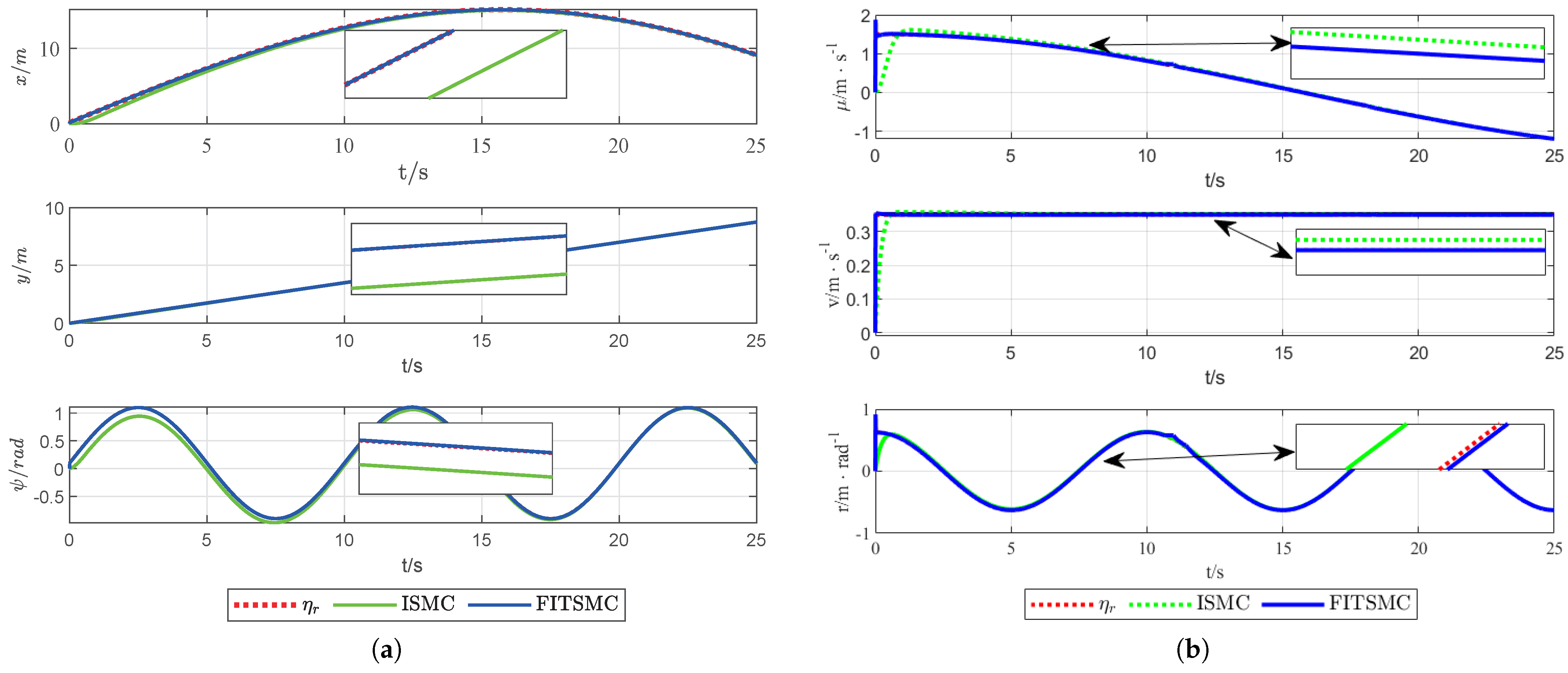
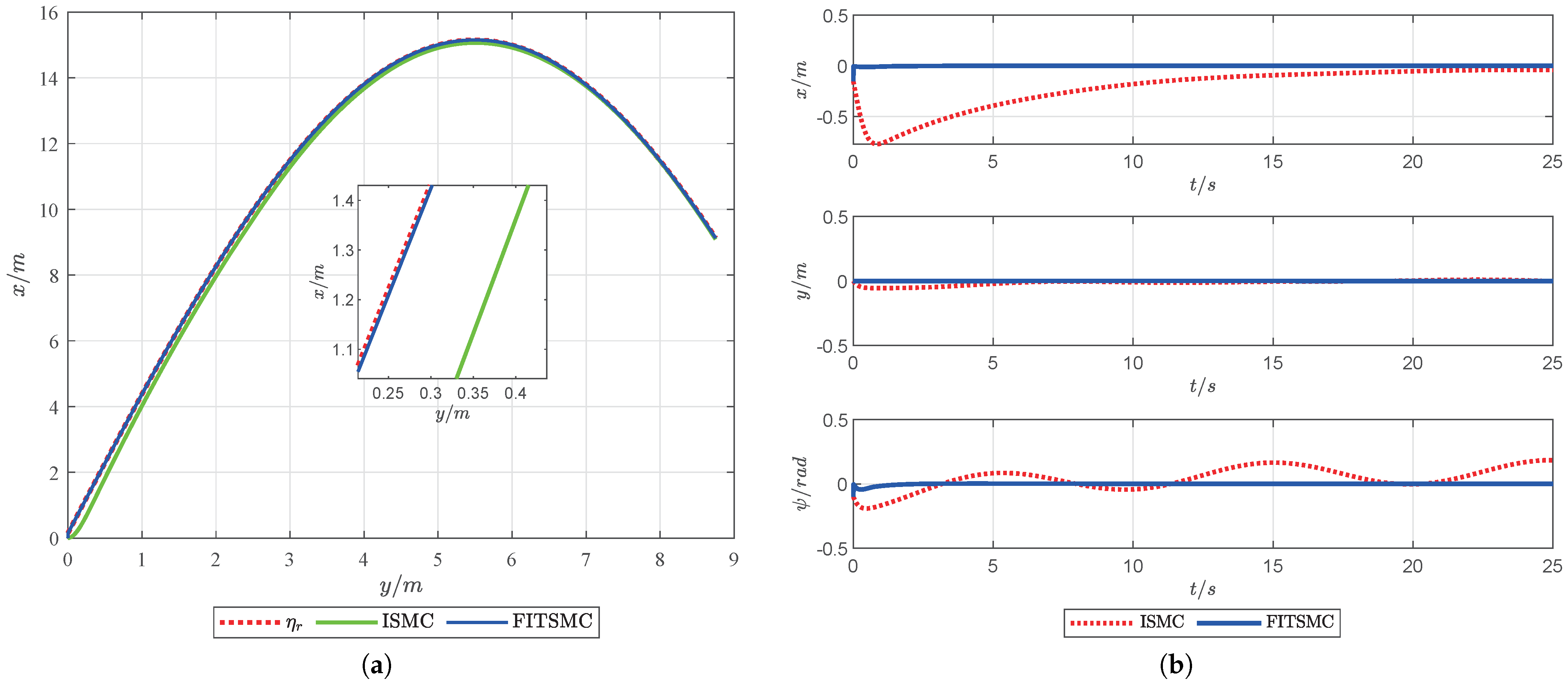
4.1. FITSMC-TTCS under Ideal Navigation State

This part provides a rigorous simulation analysis of the effectiveness of the proposed FITSMC-TTCS under ideal navigation conditions. The designed parameters of FITSMC are as follows: ${\mathrm{c}}_1=0.07$, ${\mathrm{c}}_2=0.03$, $\epsilon =15$, $k=450$, $\beta =0.15$, $\xi =0.06$, ${\Delta }_1$ = 0.01, ${\Delta }_2$ = 0.35, $\alpha$ = 0.60. The parameters of ISMC are the same as those of FITSMC-TTCS. The selected desired tracking trajectory is ${\eta }_d={[15\ast sin(0.1\ast t)+0.15,0.35\ast t,sin(0.63\ast t)+0.1]}^T$.

The specific simulation analysis is shown in Figure 2 and Figure 3. Specifically, Figure 2a represents the navigation trajectory of the USV under ISMC and FITSMC, and Figure 2b represents the trajectory error curve of the USV under an ideal navigation state based on ISMC and FITSMC. Observations from Figure 2 elucidate that while both ISMC and FITSMC are capable of effectively tracking the predetermined trajectory, FITSMC exhibits superiority by tracking the desired trajectory with minimal errors in a shorter time. Figure 3 shows the trajectory tracking curve and velocity tracking curve in the x, y, and $\psi$ directions, where Figure 3a visualizes the trajectory tracking performance, and Figure 3b outlines the velocity tracking efficiency. It is apparent that the FITSMC strategy attains the desired position and velocity swiftly and with higher tracking precision.

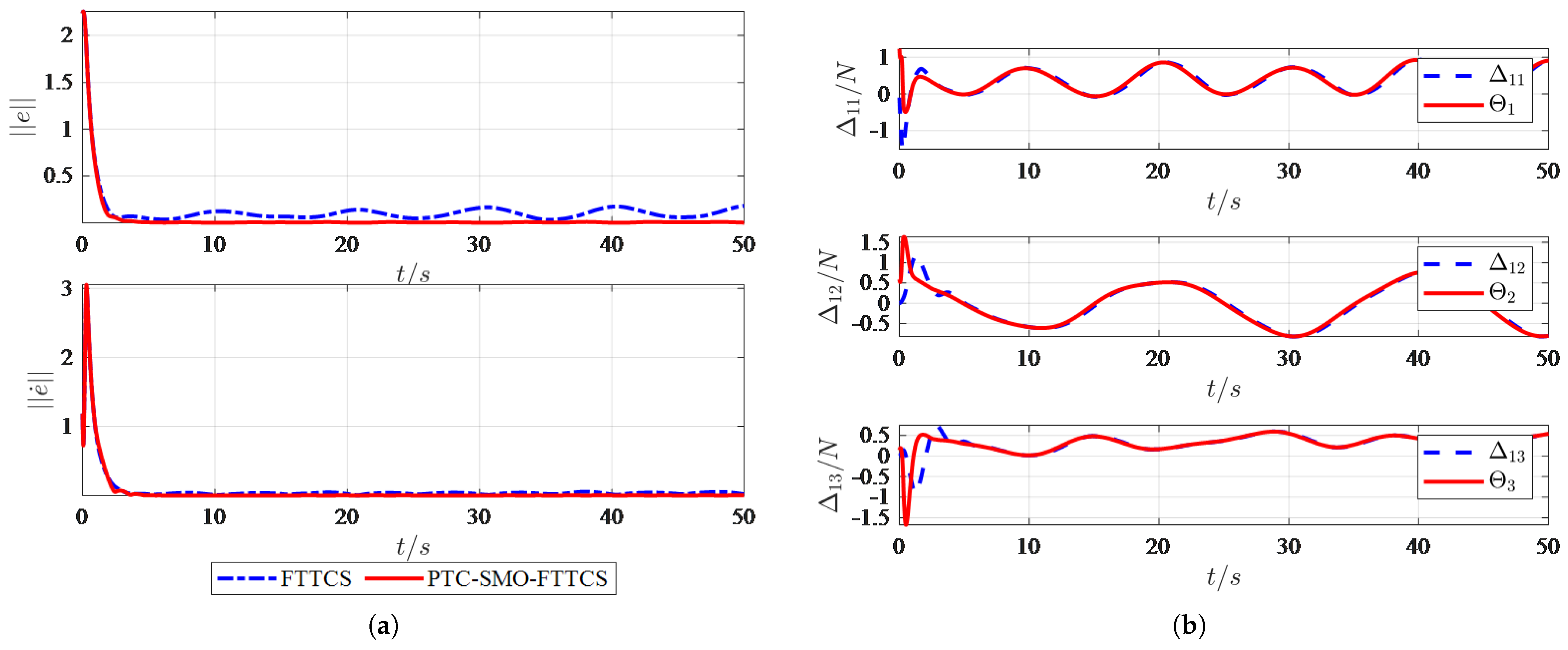
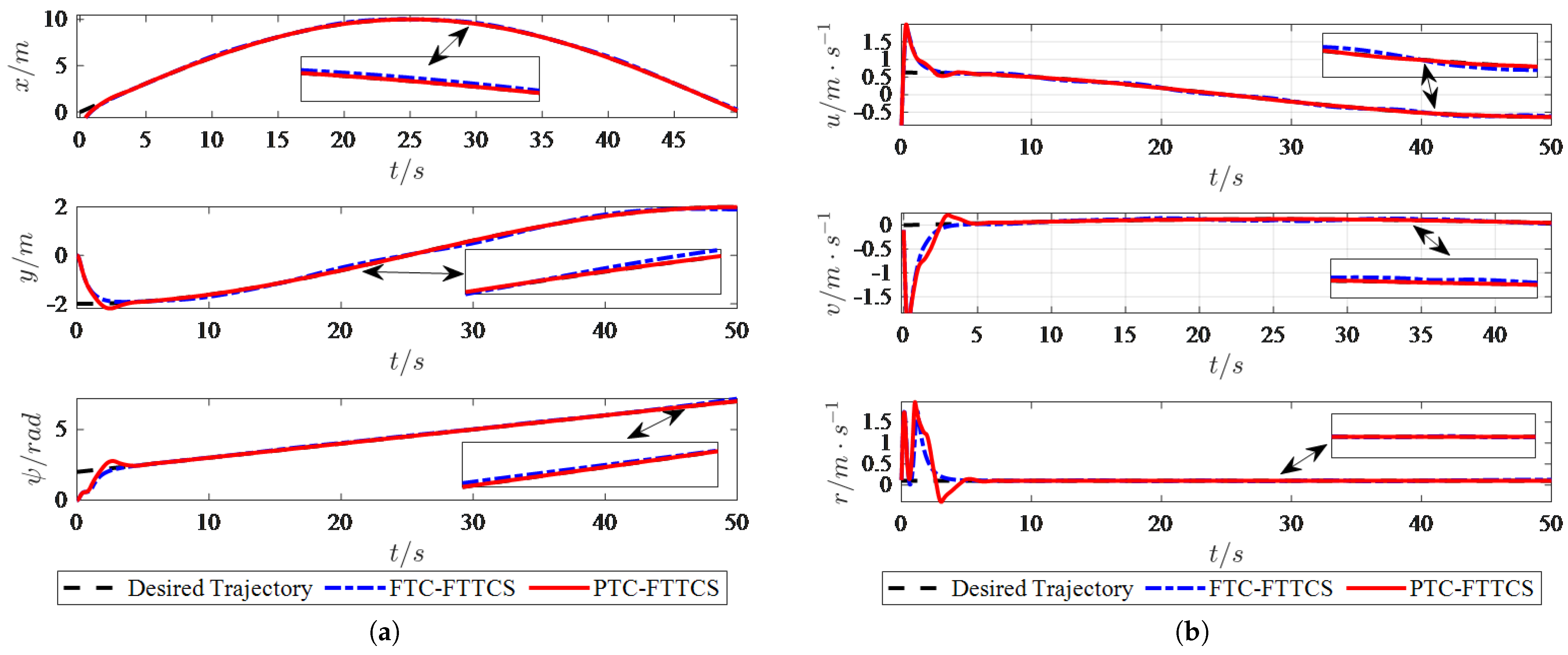
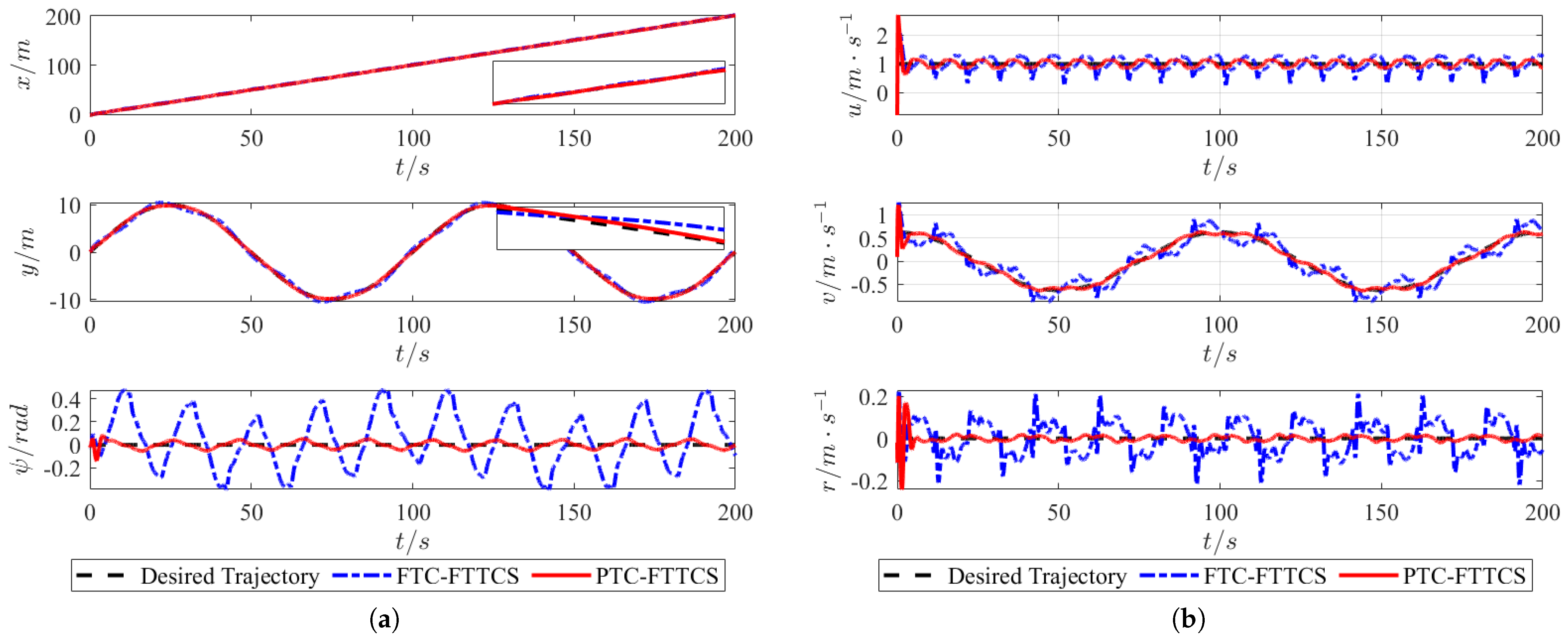
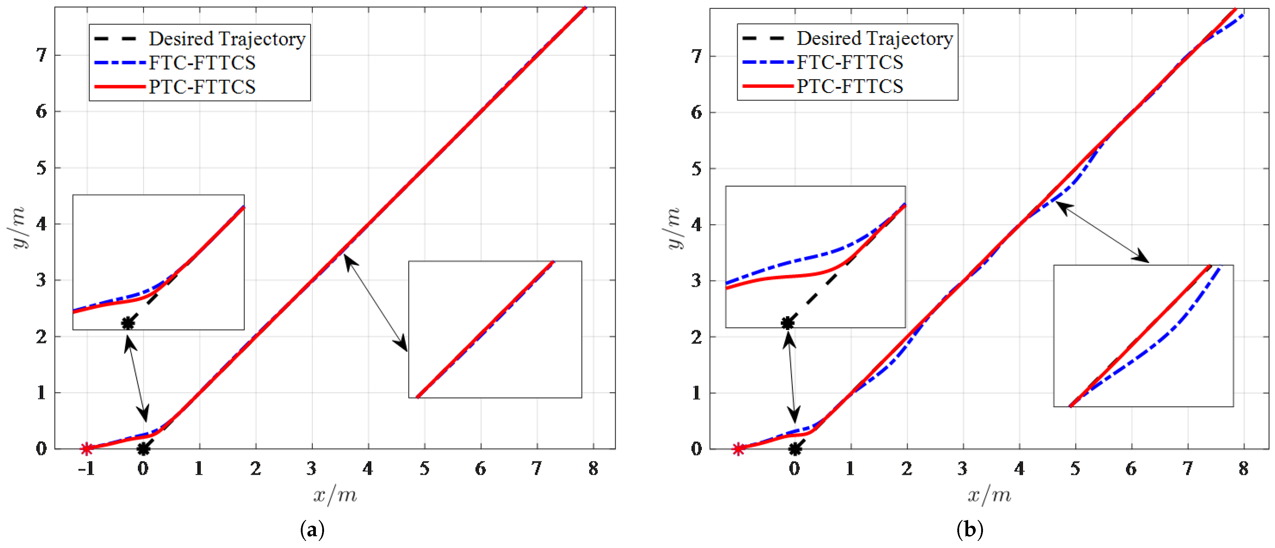
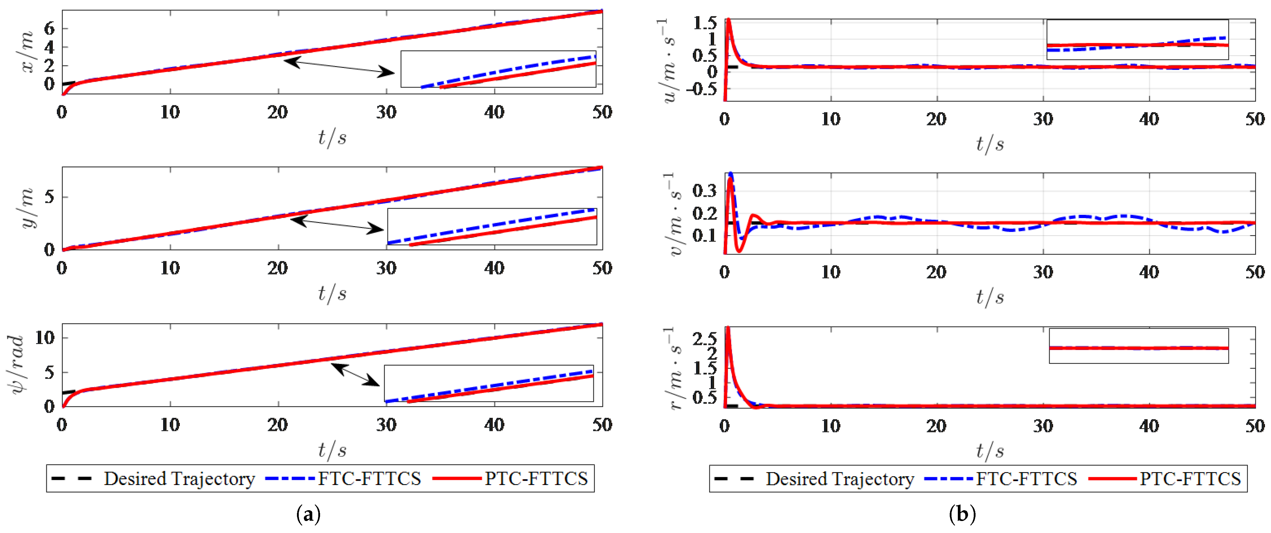
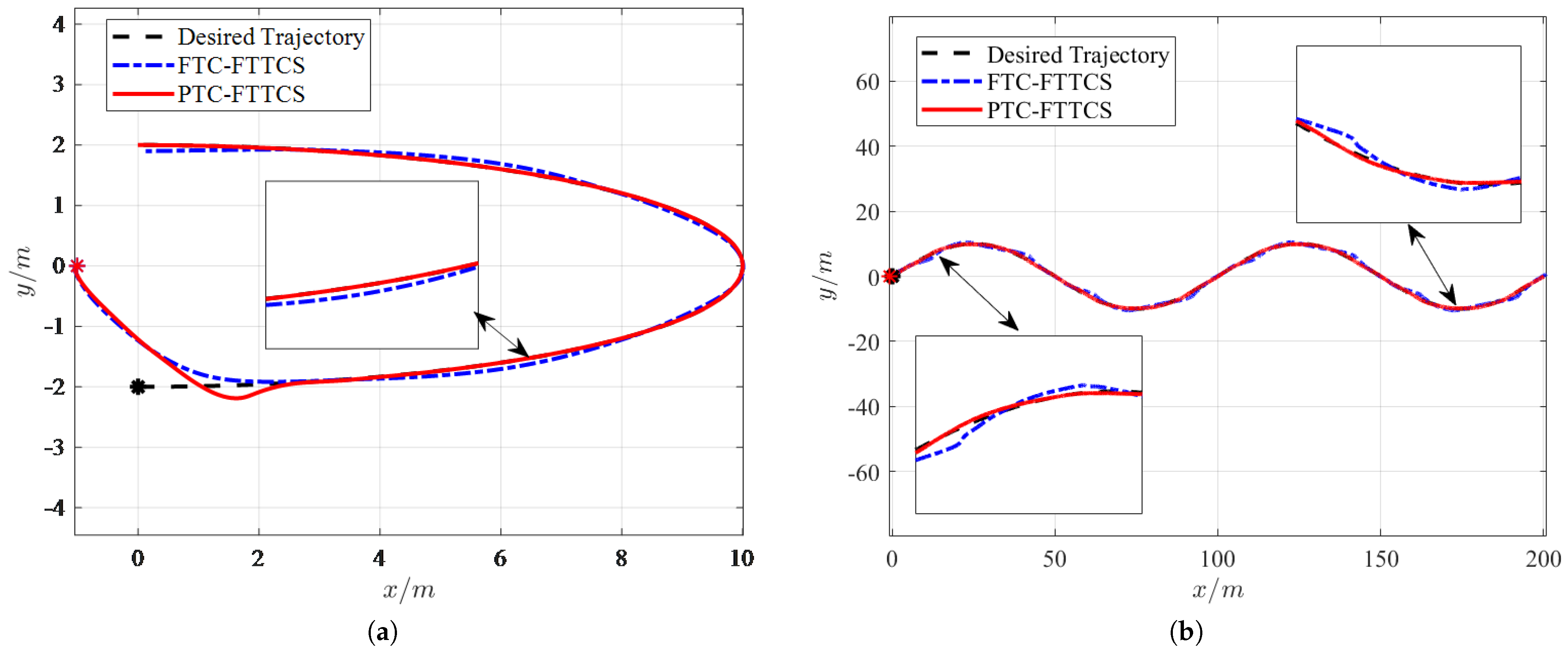
4.2. PTC-FTTCS and PTO-SMO with Complex Disturbances

During the actual navigation process, the USV confronts formidable challenges due to complex external disturbances, which significantly impede the precision of tracking control. On the basis of FITSMC-TTCS under ideal navigation conditions, this part conducts a comprehensive comparative simulation with existing fixed-time convergence algorithms [32] to further verify the efficiency of the proposed PTC-FTTCS and PTO-SMO. Specifically, the designed PTC-FTTCS and PTO-SMO parameters are shown in

Table 3. The designed PTC-FTTCs and PTO-SMO parameters.

Parm	Setvalue	Parm	Setvalue	Parm	Setvalue
$\gamma$	2	$T_{d1}$	$1.0$ s	${\beta }_1$	1200
k	1	$T_{d2}$	$0.05$ s	${\beta }_2$	−5.870
$m({\xi }_p\ne 0,{\xi }_1=0)$	1	$m\left(\mathrm{other}\right)$	$0.5$	$\widehat{L}$	2000

.

The specific simulation analysis is shown in Figure 4, Figure 5, Figure 6, Figure 7, Figure 8 and Figure 9. Firstly, two sets of comparative simulations are conducted with FTC-FTTCS to evaluate the efficacy of the introduced PTO-FTTCS, as shown in Figure 4. The selected desired tracking trajectory is ${\eta }_d={[0.05\pi t,0.05\pi t,0.2t+2]}^T$. Specifically, under both constant and time-varying disturbances, the designed PTO-FTTCS can control the USV to move along the set expected path stably, while FTC-FTTCS fails to effectively follow the set path in the presence of time-varying disturbances, proving the effectiveness of PTO-FTTCS. Moreover, the comprehensive tracking performance is further elucidated through detailed position and velocity tracking curves presented in Figure 5, which further demonstrate that the proposed PTO-FTTCS can achieve accurate tracking performance in different dimensions, and the tracking time satisfies the predefined time set.

Figure 6 substantiates the observation capability of the introduced PTC-SMO. Specifically, from Figure 6a, it can be seen that PTC-SMO can achieve precise observations of complex disturbances, ensuring that disturbance observation errors converge to 0 within predefined times. The time-varying disturbance dynamic tracking curve in Figure 6b further demonstrates the global effectiveness of PTC-SMO. Subsequently, two series of curve trajectory expansion experiments are executed to further validate the reliability of the proposed PTC-FTTCS algorithm. In Figure 7, the developed PTC-FTTCS demonstrates its proficiency in facilitating the swift and consistent tracking along the expected elliptical trajectory ${\eta }_d$ = ${[10sin\left(0.02\pi t\right),-2cos\left(0.02\pi t\right),0.1t+2]}^T$ and wave trajectory ${\eta }_d$ = ${[t,10sin\left(0.02\pi t\right),0]}^T$. The proposed algorithm is further corroborated by the exhaustive analysis of position and velocity tracking effects delineated in Figure 8 and Figure 9.

In summary, through the rigorous numerical simulation comparison and verification mentioned above, it is concluded that the tracking performance of the FITSMC-TTCS under an ideal navigation state and the PTC-FTTCS with complex disturbances proposed in this paper is superior to the state-of-the-art methods and the proposed PTO-SMO can achieve precise observation of time-varying disturbances in global time.

5. Conclusions

Addressing the intricate challenge of precise tracking control under time-varying disturbances, this paper combines the fast integral terminal sliding mode, predefined time convergence theory, and disturbance observer technology to significantly improve trajectory tracking performance from three aspects. Firstly, a novel FITSMC trajectory tracking control strategy is proposed, ensuring rapid and stable tracking of the desired trajectory under ideal navigation conditions in finite time. Following this, global stable observation of time-varying disturbances is achieved through the proposed PTC-SMO, effectively eliminating the influence of lumped disturbances on tracking control accuracy. Furthermore, the PTC-FTTCS ensures the tracking system’s state transitions to a vicinity near the origin within a predefined time. Finally, the efficiency of the proposed algorithms in this paper is proven through rigorous numerical comparison and simulation.

The algorithm proposed in this article provides a novel approach for subsequent multi-USVs cooperative trajectory tracking and formation control problems. When the physical verification conditions are met in the future, we will further verify the proposed algorithms in this paper through physical experiments.

References

1. Campbell, S.; Naeem, W.; Irwin, G.W. A review on improving the autonomy of unmanned surface vehicles through intelligent collision avoidance manoeuvres. Annu. Rev. Control 2012, 36, 267–283. [Google Scholar] [CrossRef]
2. Liu, Z.; Zhang, Y.; Yu, X.; Yuan, C. Unmanned surface vehicles: An overview of developments and challenges. Annu. Rev. Control 2016, 41, 71–93. [Google Scholar] [CrossRef]
3. Abdelaal, M.; Fränzle, M.; Hahn, A. Nonlinear Model Predictive Control for trajectory tracking and collision avoidance of underactuated vessels with disturbances. Ocean. Eng. 2018, 160, 168–180. [Google Scholar] [CrossRef]
4. Sun, X.J.; Wang, G.F.; Fan, Y.S. Adaptive trajectory tracking control of vector propulsion unmanned surface vehicle with disturbances and input saturation. Nonlinear Dyn. 2021, 106, 2277–2291. [Google Scholar] [CrossRef]
5. Mu, D.D.; Wang, G.F.; Fan, Y.S.; Qiu, B.B.; Sun, X.J. Adaptive Trajectory Tracking Control for Underactuated Unmanned Surface Vehicle Subject to Unknown Dynamics and Time-Varing Disturbances. Appl. Sci. 2018, 8, 547. [Google Scholar] [CrossRef]
6. Gonzalez-Garcia, A.; Castañeda, H.; Garrido, L. USV Path-Following Control Based On Deep Reinforcement Learning and Adaptive Control. In Proceedings of the Global Oceans 2020, Biloxi, MS, USA, 5–30 October 2020. [Google Scholar] [CrossRef]
7. Feng, K.; Wang, N.; Liu, D.; Er, M.J. Adaptive Fuzzy Trajectory Tracking Control of Unmanned Surface Vehicles with Unknown Dynamics. In Proceedings of the IEEE 3rd International Conference on Informative and Cybernetics for Computational Social Systems, Jinzhou, China, 26–29 August 2016; pp. 342–347. [Google Scholar]
8. Fan, Y.S.; Sun, X.J.; Wang, G.F.; Guo, C. On Fuzzy Self-adaptive PID Control for USV Course. In Proceedings of the 2015 34th Chinese Control Conference, Hangzhou, China, 28–30 July 2015; pp. 8472–8478. [Google Scholar]
9. Mu, D.D.; Wang, G.F.; Fan, Y.S.; Sun, X.J.; Qiu, B.B. Adaptive LOS Path Following for a Podded Propulsion Unmanned Surface Vehicle with Uncertainty of Model and Actuator Saturation. Appl. Sci. 2017, 7, 1232. [Google Scholar] [CrossRef]
10. Zhou, B.; Huang, B.; Su, Y.M.; Zheng, Y.X.; Zheng, S. Fixed-time neural network trajectory tracking control for underactuated surface vessels. Ocean. Eng. 2021, 236, 109416. [Google Scholar] [CrossRef]
11. Zhao, Y.J.; Qi, X.; Ma, Y.; Li, Z.X.; Malekian, R.; Sotelo, M.A. Path Following Optimization for an Underactuated USV Using Smoothly-Convergent Deep Reinforcement Learning. IEEE Trans. Intell. Transp. Syst. 2021, 22, 6208–6220. [Google Scholar] [CrossRef]
12. Gonzalez-Garcia, A.; Castañeda, H. Guidance and Control Based on Adaptive Sliding Mode Strategy for a USV Subject to Uncertainties. IEEE J. Ocean. Eng. 2021, 46, 1144–1154. [Google Scholar] [CrossRef]
13. Yu, Y.L.; Guo, C.; Yu, H.M. Finite-Time PLOS-Based Integral Sliding-Mode Adaptive Neural Path Following for Unmanned Surface Vessels With Unknown Dynamics and Disturbances. IEEE Trans. Autom. Sci. Eng. 2019, 16, 1500–1511. [Google Scholar] [CrossRef]
14. Qu, X.R.; Liang, X.; Hou, Y.H.; Li, Y.; Zhang, R.B. Path-following control of unmanned surface vehicles with unknown dynamics and unmeasured velocities. J. Mar. Sci. Technol. 2021, 26, 395–407. [Google Scholar] [CrossRef]
15. Chen, X.; Liu, Z.; Zhang, J.Q.; Zhou, D.C.; Dong, J. Adaptive sliding-mode path following control system of the underactuated USV under the influence of ocean currents. J. Syst. Eng. Electron. 2018, 29, 1271–1283. [Google Scholar] [CrossRef]
16. Wang, D.; Kong, M.; Zhang, G.; Liang, X. Adaptive second-order fast terminal sliding-mode formation control for unmanned surface vehicles. J. Mar. Sci. Eng. 2022, 10, 1782. [Google Scholar] [CrossRef]
17. Fan, Z.P.; Xu, Y.J.; Fu, M.Y. Finite-time command filtered backstepping control for USV path following. Automatica 2023, 92, 173–180. [Google Scholar] [CrossRef]
18. Ghommam, J.; Saad, M.; Mnif, F.; Zhu, Q.M. Guaranteed Performance Design for Formation Tracking and Collision Avoidance of Multiple USVs With Disturbances and Unmodeled Dynamics. IEEE Syst. J. 2021, 15, 4346–4357. [Google Scholar] [CrossRef]
19. Sánchez-Tones, J.D.; Sanchez, E.N.; Loukianov, A.G. Predefined-Time Stability of Dynamical Systems with Sliding Modes. In Proceedings of the 2015 American Control Conference, Chicago, IL, USA, 1–3 July 2015; pp. 5842–5846. [Google Scholar]
20. Becerra, H.M.; Vázquez, C.R.; Arechavaleta, G.; Delfin, J. Predefined-Time Convergence Control for High-Order Integrator Systems Using Time Base Generators. IEEE Trans. Control. Syst. Technol. 2018, 26, 1866–1873. [Google Scholar] [CrossRef]
21. Yang, Y.Q.; Ge, M.F.; Liang, C.D.; Xu, K.T.; Wang, L. Predefined-time formation control of NASVs with fully discontinuous communication: A novel hierarchical event-triggered scheme. Ocean. Eng. 2023, 268, 113422. [Google Scholar] [CrossRef]
22. Liang, C.D.; Ge, M.F.; Liu, Z.W.; Gu, Z.W.; Chen, Q. Distributed predefined-time optimization control for networked marine surface vehicles subject to set constraints. IEEE Trans. Intell. Transp. Syst. 2023, 25, 2129–2138. [Google Scholar] [CrossRef]
23. Liang, C.D.; Ge, M.F.; Liu, Z.W.; Ling, G.; Liu, F. Predefined-time formation tracking control of networked marine surface vehicles. Control Eng. Pract. 2021, 107, 104682. [Google Scholar] [CrossRef]
24. Li, M.C.; Guo, C.; Yu, H.M. Filtered Extended State Observer Based Line-of-Sight Guidance for Path Following of Unmanned Surface Vehicles with Unknown Dynamics and Disturbances. IEEE Access 2019, 7, 178401–178412. [Google Scholar] [CrossRef]
25. Wu, G.X.; Ding, Y.; Tahsin, T.; Atilla, I. Adaptive neural network and extended state observer-based non-singular terminal sliding modetracking control for an underactuated USV with unknown uncertainties. Appl. Ocean. Res. 2023, 135, 103560. [Google Scholar] [CrossRef]
26. Li, X.S.; Li, X.C.; Ma, D.G.; Kong, X.W. Trajectory Tracking Control of Unmanned Surface Vehicles Based on a Fixed-Time Disturbance Observer. Electronics 2023, 12, 2896. [Google Scholar] [CrossRef]
27. Song, J.; Niu, Y.G.; Zou, Y.Y. Finite-Time Stabilization via Sliding Mode Control. IEEE Trans. Autom. Control. 2017, 62, 1478–1483. [Google Scholar] [CrossRef]
28. Moulay, E.; Lechappe, V.; Bernuau, E.; Defoort, M.; Plestan, F. Fixed-time sliding mode control with mismatched disturbances. Automatica 2022, 136, 110009. [Google Scholar] [CrossRef]
29. Liu, Y.C.; Yan, W.; Zhang, T.; Yu, C.X.; Tu, H.Y. Trajectory Tracking for a Dual-Arm Free-Floating Space Robot With a Class of General Nonsingular Predefined-Time Terminal Sliding Mode. IEEE Trans. Syst. Man Cybern. Syst. 2022, 52, 3273–3286. [Google Scholar] [CrossRef]
30. Wu, C.H.; Yan, J.G.; Shen, J.H.; Wu, X.W.; Xiao, B. Predefined-Time Attitude Stabilization of Receiver Aircraft in Aerial Refueling. IEEE Trans. Circuits Syst. Express Briefs 2021, 68, 3321–3325. [Google Scholar] [CrossRef]
31. Skjetne, R.; Smogeli, ∅.; Fossen, T.I. Modeling, identification, and adaptive maneuvering of Cybership II: A complete design with experiments. IFAC Proc. Vol. 2004, 37, 203–208. [Google Scholar] [CrossRef]
32. Er, M.J.; Li, Z.K. Formation Control of Unmanned Surface Vehicles Using Fixed-Time Non-Singular Terminal Sliding Mode Strategy. J. Mar. Sci. Eng. 2022, 10, 1308. [Google Scholar] [CrossRef]
Figure 1. Three-degree-of-freedom USV inertial coordinate and fixed-body coordinate system.
Electronics 13 01510 g001
Figure 2. (a) Trajectory tracking curve under ideal navigation state based on ISMC and FITSMC; (b) Tracking error curve under ideal navigation state based on ISMC and FITSMC.
Electronics 13 01510 g002
Figure 3. (a) Position tracking curve based on ISMC and FITSMC; (b) Velocity tracking curve based on ISMC and FITSMC.
Electronics 13 01510 g003
Figure 4. (a) Straight trajectory tracking curve with constant complex disturbances Θ = [ 5 , 5 , 5 ] T based on FTC-FTTCS and PTC-FTTCS; (b) traight trajectory tracking curve with variable complex disturbances Θ = [ 24 cos ( 0.1 π t ) 2 , 20 cos ( 0.1 π t ) , 3 cos ( 0.3 π ) 2 ] T based on FTC-FTTCS and PTC-FTTCS.
Electronics 13 01510 g004
Figure 5. (a) Position tracking curve based on FTC-FTTCS and PTC-FTTCS; (b) Velocity tracking curve based on FTC-FTTCS and PTC-FTTCS.
Electronics 13 01510 g005
Figure 6. (a) Disturbances observation performance curve based on PTC-SMO; (b) Disturbances observation error curve based on PTC-SMO.
Electronics 13 01510 g006
Figure 7. (a) Elliptical trajectory tracking curve with variable complex disturbances Θ = [ 200 cos ( 0.1 π t ) 2 , 200 cos ( 0.1 π t ) , 3 cos ( 0.3 π ) 2 ] T based on FTC-FTTCS and PTC-FTTCS; (b) Wave trajectory tracking curve with variable complex disturbances Θ = [ 200 cos ( 0.1 π t ) 2 , 200 cos ( 0.1 π t ) , 3 cos ( 0.3 π ) 2 ] T based on FTC-FTTCS and PTC-FTTCS.
Electronics 13 01510 g007
Figure 8. (a) Position tracking curve of elliptical trajectory; (b) Velocity tracking curve of elliptical trajectory.
Electronics 13 01510 g008
Figure 9. (a) Position tracking curve of wave trajectory; (b) Velocity tracking curve of wave trajectory.
Electronics 13 01510 g009