Complexity Reduction for Converter-Driven Stability Analysis in Transmission Systems

Abstract

The high penetration of power electronic converters with complex control systems is changing the power system dynamics, introducing new challenges such as converter-driven stability incidents. Traditional stability analysis methods, suitable for classical problems like voltage, frequency, and rotor angle stability in large systems, are insufficient for addressing the fast control dynamics of converters, which involve electromagnetic phenomena. These phenomena require detailed converter and network modeling, which can be performed in both the frequency and time domains, enabling the respective stability analyses to be carried out. However, frequency domain methods, based on small-signal impedances linearized at a single operating point, inherently ignore time domain phenomena like switching events and nonlinear behaviors. In contrast, time domain electromagnetic transient (EMT) simulations are effective for analyzing converter-driven stability but are computationally intensive when applied to large transmission systems with numerous use cases. Therefore, to reduce the simulation complexity in EMT tools, a complexity reduction procedure is proposed in this paper. Leveraging the advantages of the frequency domain, such as faster simulation times and information on wideband frequency characteristics of the system, this procedure utilizes the small-signal impedances and introduces a method for network reduction. The procedure also uses the frequency domain stability analysis method to screen for critical network use cases. Primarily, this procedure is a frequency domain toolchain encompassing frequency domain stability analysis and frequency domain network reduction. The result of the toolchain is a reduced network size and reduced network use cases that can be used for EMT simulations. The procedure is applied to an IEEE 39 bus system, where converter-driven stability is evaluated for two use cases. Furthermore, the network reduction method is tested on a critical use case, demonstrating reductions in network size and computation times without compromising the quality of stability analysis results.

1. Introduction

Power system stability is a fundamental prerequisite for a secure grid operation. Power systems are complex networks with a large number of dynamic components and can be subjected to stability issues such as frequency stability, voltage stability, and rotor-angle stability [1]. However, there is currently a rapid shift in power generation from conventional power plants to renewable energy sources to achieve the goal of climate neutrality. This has resulted in an increased integration of power electronic converters in the framework of power generation, transmission, and compensation. Power electronics converters have complex control systems, consequently changing the power system dynamics. This is leading to new instability phenomena, such as converter-driven stability in the network [2].

In recent years, several converter-driven stability incidents have been reported that resulted in the shutdown of large converter stations. For example, in 2013, oscillations in the grid current and voltages at frequencies other than 50 Hz resulted in the tripping of the BorWin1 HVDC system, which connects an offshore wind farm by an islanded offshore AC grid [3]. Such instabilities are a result of interactions between multiple converters or between converter and network resonances. As the integration of converters into power systems increases, the importance of addressing these instabilities will grow. Therefore, a thorough analysis of these phenomena is crucial before installing new converters [4].

Generally, existing analysis techniques, such as root mean square (RMS) balanced simulations, are employed to carry out classical stability studies. RMS simulations are phasor domain transient (PDT) simulations, which are valid for simulating electromechanical phenomena ranging from inertial response to frequency control. They operate on the assumption that the system is balanced and is operating at the fundamental frequency. In most cases, the power system is designed as a positive sequence equivalent circuit. The sinusoidal quantities, such as voltages and currents, are represented as phasors rotating at the fundamental frequency and as DC quantities in steady state. The network elements, such as transmission lines, are represented using their corresponding impedance at the system’s fundamental frequency [4,5]. These significant simplifications accommodate variable step solvers, leading to easier simulation of large networks of up to several thousand buses [6]. However, sufficient detail to analyze fast dynamic phenomena such as converter-driven stability cannot be achieved through these approximated simulations.

One of the widely used methods for converter-driven stability analysis is an impedance-based stability analysis method [7]. This is a small-signal stability analysis method that uses classical control theory tools such as Nyquist and Bode plots. This method has been applied initially to analyze interactions between a single converter system and a simplified AC grid. For analyzing multiple converter systems, this method has been extensively studied for wind farms with converter-based wind turbines. It has been observed that the aggregation of converters is not adequate. Therefore, various iterative approaches have been considered to carry out the analysis [8]. Additionally, comparative studies of methods to analyze radial networks have been conducted [9]. Only in recent years, a few methods for frequency domain impedance-based analysis have been investigated for meshed networks. Additionally, the applicability of these methods has been investigated and compared, considering black-box converter impedance models [10]. However, the meshed networks used for analysis are smaller networks, such as 3-bus networks and 6-bus networks, and their robustness on bigger networks is not investigated.

Furthermore, this method operates in the frequency domain where the transformation of any casual linear time-invariant (LTI) system results in algebraic equations that are easier to solve. Therefore, this frequency domain method is suitable for analyzing numerous grid use cases. However, in this method, the system model is linearized at a single operating point. As power electronic devices are non-linear entities, a linearized approach such as this can have limitations for the analysis. Therefore, a more adequate tool is required where the electromagnetic transients in the network can be rightly represented.

Electromagnetic transient (EMT) simulation tools, as the name suggests, can be employed for converter-driven stability analysis. Unlike RMS simulation tools, which are based on simplified mathematical representations, EMT is a time domain tool that does not undergo inherent simplifications and, therefore, captures the instantaneous voltage and current waveforms. Power electronic interfaced devices require instantaneous voltage and current as input to control systems for their operation [4]. Additionally, the availability of detailed three-phase component models, such as transmission lines, makes this a suitable simulation environment. Subsequently, the accuracy of results obtained is only limited to the parameter data available and the computing power. However, the simulation times can be excessive due to the small simulation time steps required by fast controllers [4,6]. Therefore, simulating large networks with numerous grid use cases is computationally cumbersome [4].

To summarize, the frequency domain modeling of meshed networks has only been investigated on small networks, considering only a few components such as lines, loads, and converters [11]. Additionally, frequency domain converter-driven stability analysis methods have been investigated only on small meshed networks such as 6-bus networks [10,11]. In contrast, time domain converter-driven stability analysis in EMT tools has been conducted on networks considering thousands of network buses, resulting in simulations that are complex and time-consuming, especially for simulating several grid use cases. Furthermore, no methods for determining boundary buses to obtain the relevant network area for converter-driven stability have been introduced [4].

Therefore, this paper utilizes a 39 bus system to investigate the validity of the frequency domain network modeling, considering lines, transformers, loads, generators, and converters. Furthermore, the frequency domain stability analysis is conducted, and its validity on a network of this size is tested. Moreover, a procedure to determine the boundary buses for obtaining relevant network areas for converter-driven stability analysis is proposed and validated. Based on the relevant boundary buses, the size of the network is reduced for further simulations in the EMT tool.

Overall, this paper presents a procedure to reduce the complexity of converter-driven stability analysis in EMT tools for transmission networks. Catering to the advantages of impedance-based analysis, a frequency domain tool is introduced for reducing the final number of grid use cases and the size of the network for analysis in the EMT tool. The procedure introduced consists of frequency domain network modeling, frequency domain stability analysis, and a frequency domain network reduction method. The final outputs of the procedure are the reduced grid use cases and a reduced network, recommended to be used for simulations in the EMT tool. This paper also takes into consideration that the future grids have multiple converter vendors, and the converter control design is the intellectual property of the manufacturer. Therefore, a third-party analysis is made possible in this procedure as it considers converter black-box models.

An overview of the proposed method is presented in Section 2. The modeling of the converter, passive components, and network admittance is presented in Section 3. Section 4 describes the frequency domain stability analysis method that is investigated. In Section 5, a method for frequency domain network reduction is introduced. Exemplary results are presented in Section 6. In Section 7, a summary and conclusions are drawn.

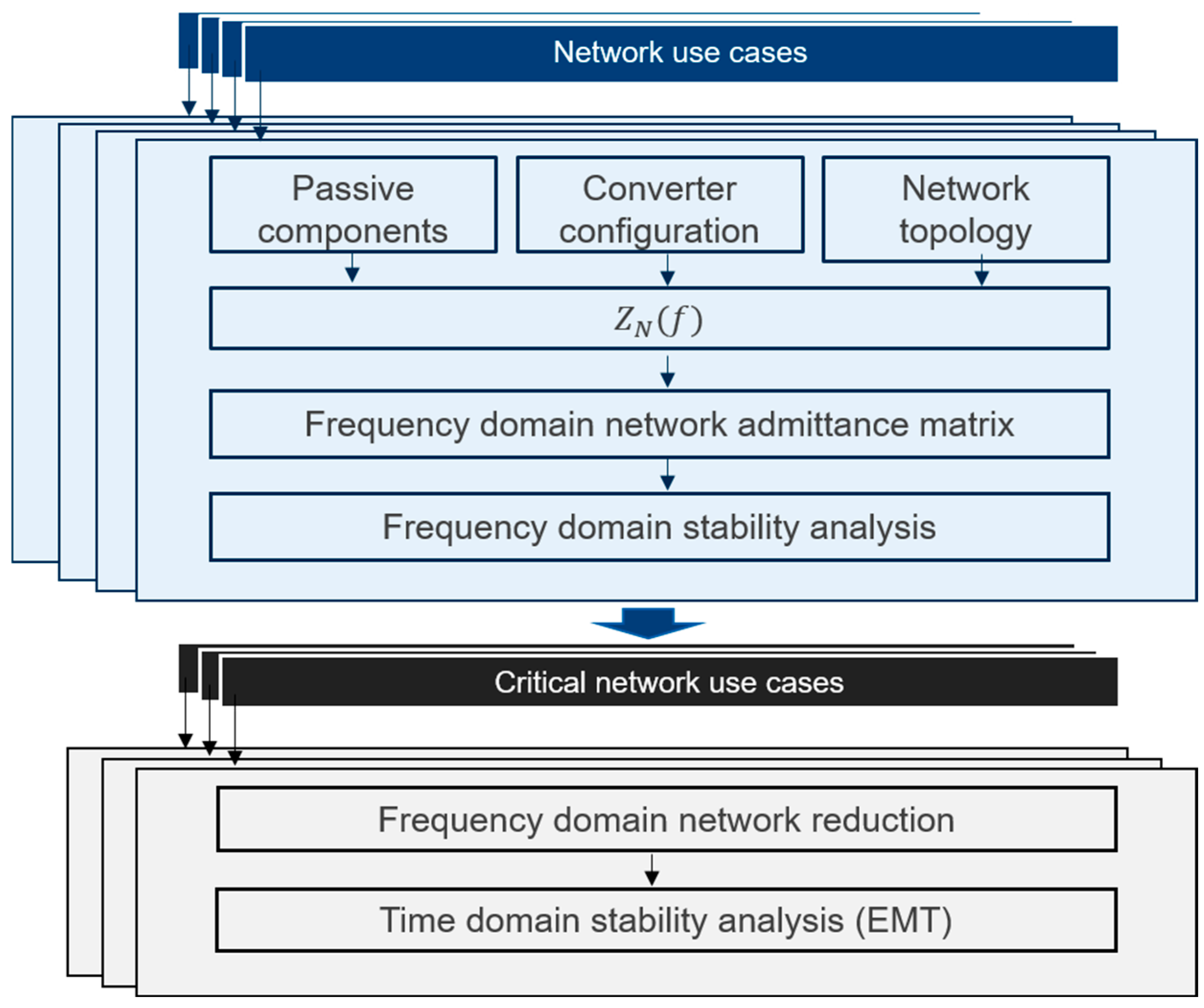
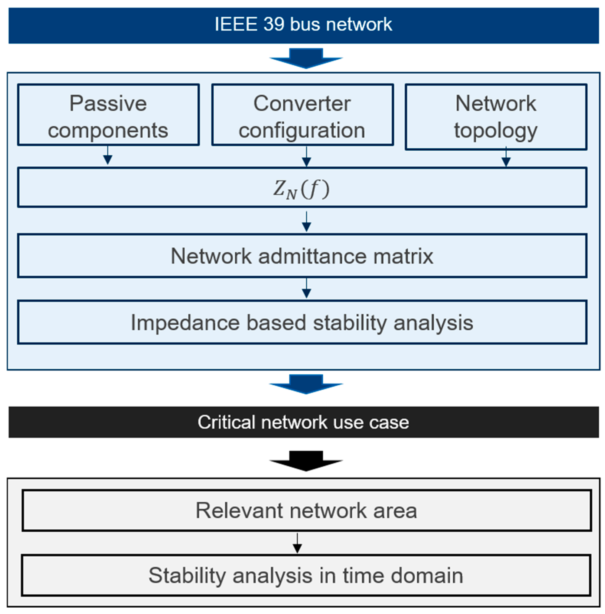
2. Overview of the Proposed Complexity Reduction Procedure

The complexity reduction procedure developed is a frequency domain procedure that prepares the network for converter-driven stability analysis in an EMT tool. The workflow of the procedure is shown in Figure 1. As shown in the Figure 1, this procedure is divided into two stages:

• Identification of critical network use cases
• Reduction of network area under study

Stage one of the procedure begins with the preparation of input data. The input consists of information on grid topology, parameter data for the passive components such as transmission lines, transformers, and passive loads, and frequency-dependent impedances of the converters in the grid. This information is required for each grid use case to be investigated. Based on the data provided, the tool prepares the individual impedances of the network components and then utilizes them for the construction of the network admittance matrix. This is performed repetitively for all the grid use cases provided. Finally, the network admittance matrix is given as an input to the frequency domain stability analysis method. The stability analysis method used is described in Section 4. The output of the frequency domain stability analysis method is a set of critical grid use cases. These critical use cases are further given as input to stage two of the procedure.

Stage two deals with the determination of the network area under study. This part of the procedure utilizes the impedance characteristics of the network and quantifies the influence of network components and the corresponding buses at the point of common coupling. Buses with the least sensitivity to the point of common coupling are reduced and replaced with power flow equivalents. The final result is a new topology of the grid use case, with a reduced number of components and buses. This new reduced system created for critical grid use cases is then utilized as an input to an EMT tool to conduct final EMT simulations. A further explanation of the frequency domain network reduction procedure is presented in Section 5.

3. Modeling of the Network and Its Components

To simulate the dynamics relevant to converter-driven stability analysis, a detailed model of the converter and the rest of the network is required. It has been observed that the wideband characteristics of a component are rightly captured by their frequency-dependent impedances and are adequate for converter-driven stability analysis. Therefore, in this section, impedance modeling of the converter and the rest of the network is briefly described.

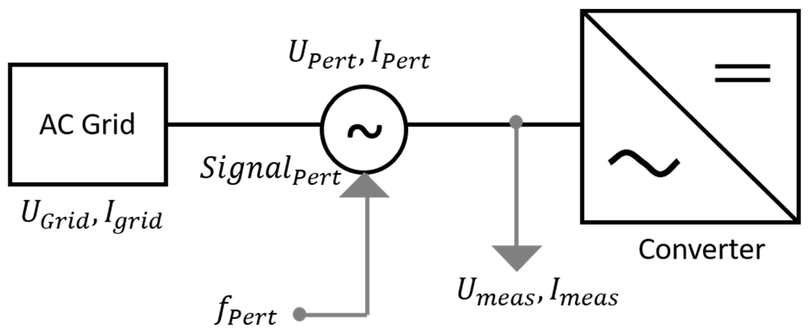
3.1. Converter Modeling

Since the converters in a grid often come from different manufacturers, a third-party evaluation may be needed to assess system stability. As a result, black-box models of converters are necessary. In accordance with VDE-AR-N 4130 [12], manufacturers are required to provide transmission system operators (TSOs) with frequency-dependent impedance models of the converters. In this paper, a numerical approach is used to obtain these impedance models, which enable the analysis of converters whose control systems and internal electrical configurations are unknown to the operator. In Figure 2, the setup for the numerical derivation of converter impedance is given. It demonstrates a perturbation injection method, which is used to numerically derive the AC-side impedance of a converter [6]. Depending on the control mode, a small-signal perturbation, either as voltage ($U_{pert})$ or current ($I_{pert})$ at different frequencies ($f_{pert} \left\{1,2\dots n\right\}),$ is given as an input. This perturbation triggers the converter’s response to these frequencies. The converter terminal voltages ${(U}_{meas})$ and currents ($I_{meas})$ are measured at the perturbation frequencies ($f_{pert} \{1,2\dots n\})$ using Fourier transforms. From these measurements, a discrete converter impedance is calculated as $z_C(f)=\left\{z_{fpert1, }\right.z_{fpert2, }\dots z_{fpertn}\}$. An inverse of this gives the nodal admittance ${(y}_C(f))$ of the converter, which is further used for the construction of the network admittance matrix.

3.2. Passive Component Modeling

Generic analytical modeling approaches found in [13,14,15] are utilized for frequency-dependent impedance modeling of the passive components. Specifically for the modeling of branch components such as transmission lines and transformers, the impedances are modeled in terms of ABCD parameters also known as transmission parameters. In this work, for the modeling of line impedances, wide-band models are utilized, considering distributed line characteristics. For wideband modeling, unlike lumped RLC parameters for a line, mirror imaging methods and Bessel functions, which consider the geometry and the electromagnetic properties of a line, are utilized for the calculation of the line parameters. The admittance matrix $Y$ and the impedance matrix $Z$ are generated based on the shunt capacitances and the internal and external series impedances of a transmission line, respectively. These are further used to formulate the ABCD parameters of the lines given by the following equations.

$$A(f)=\cosh \left(\sqrt{Y\left(f\right)\cdot Z\left(f\right)}\cdot l\right)$$

(1)

$$B(f)=\sqrt{{\displaystyle \frac{Z\left(f\right)}{Y\left(f\right)}}}\sinh \left(\sqrt{Y\left(f\right)\cdot Z\left(f\right)}\cdot l\right)$$

(2)

$$C(f)=\sinh \left(\sqrt{Y\left(f\right)\cdot Z\left(f\right)}\cdot l\right)\sqrt{{\displaystyle \frac{Y\left(f\right)}{Z\left(f\right)}}}$$

(3)

$$D\left(f\right)=A\left(f\right)$$

(4)

The frequency-dependent impedance of the transformer is modeled based on its equivalent circuit considering the primary side $(p)$, secondary side $(s),$ and shunt magnetizing ($m)$ reactance and resistance. The ABCD parameters of the transformers are given by the following equations.

$$A(f)=n\left\{1+\left(R_p+j\omega L_p\right)\left({\displaystyle \frac{1}{R_m}}+{\displaystyle \frac{1}{j\omega L_m}}\right)\right\}$$

(5)

$$B(f)=n\left\{1+\left(R_p+j\omega L_p\right)\left({\displaystyle \frac{1}{R_m}}+{\displaystyle \frac{1}{j\omega L_m}}\right)\right\}\left(R_s+j\omega L_s\right)+{\displaystyle \frac{1}{n}}\left(R_p+j\omega L_p\right)$$

(6)

$$C(f)=n\left({\displaystyle \frac{1}{R_m}}+{\displaystyle \frac{1}{j\omega L_m}}\right)$$

(7)

$$D(f)=n\left({\displaystyle \frac{1}{R_m}}+{\displaystyle \frac{1}{j\omega L_m}}\right)\left(R_s+j\omega L_s\right)+{\displaystyle \frac{1}{n}}$$

(8)

Additionally, the impedances of the transformers are modeled without considering stray capacitances. The nodal components, such as loads, are directly modeled as admittances. According to the active and reactive power demand at a bus, the load impedances are modeled as parallel RLC circuits. The generators are modeled as impedances with dominating inductive characteristics. Analytical models are initially modeled as continuous transfer functions but are adapted to match the discrete converter data by representing the continuous models as a discrete set of impedance data points over a specific frequency range.

3.3. Network Modeling

Finally, using the admittances of converter and passive components and the network topology, a frequency-dependent network admittance matrix is formulated according to Equation (9). Based on ref. [11], the diagonal element of the network admittance matrix for a bus $i$ is given by the summation of all the nodal and branch components connected to bus $i$. The admittances ($y_i\left(f\right))$ of nodal components are used directly, whereas the admittances of the branch components are represented in terms of ABCD parameters. The A and B parameters of $k$ transmission lines connected to bus $i$ are given by $A_{Lik}\left(f\right)$ and $B_{Lik}\left(f\right)$. Given that the transformer primary side is connected to bus $i$, the branch admittance is given by $A_{Tik}\left(f\right)$ and $B_{Tik}\left(f\right)$, and in the case of the transformer secondary side being connected to bus $i$, the branch admittance is given by $D_{Tik}\left(f\right)$ and $B_{Tik}\left(f\right)$. The non-diagonal elements of the matrix are given by the branch elements connected between bus $i$ and other buses, which are represented in the admittance matrix by $-{\displaystyle \frac{1}{B_{ik}\left(f\right)}}$. Unlike diagonal elements, the term used in this case is the same for both transmission lines and transformers.

$$Y_{ij}\left(f\right)=\left\{\begin{array}{c}{\displaystyle \sum _k}{y}_{ik}\left(f\right)+{\displaystyle \sum _k}{\displaystyle \frac{A_{Lik}\left(f\right)}{B_{Lik}\left(f\right)}}+\left\{\begin{array}{c}{\displaystyle \sum _k}{\displaystyle \frac{A_{Tik}\left(f\right)}{B_{Tik}\left(f\right)}}if i connected to primary side\\ {\displaystyle \sum _k}{\displaystyle \frac{D_{Tik}\left(f\right)}{B_{Tik}\left(f\right)}}if i connected to secondary side\end{array}if i=j\right.\\ -{\displaystyle \frac{1}{B_{ik}\left(f\right)}} if i\ne j \end{array}\right\}$$

(9)

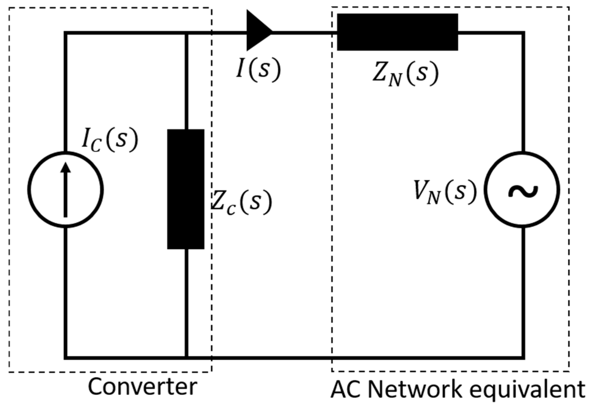
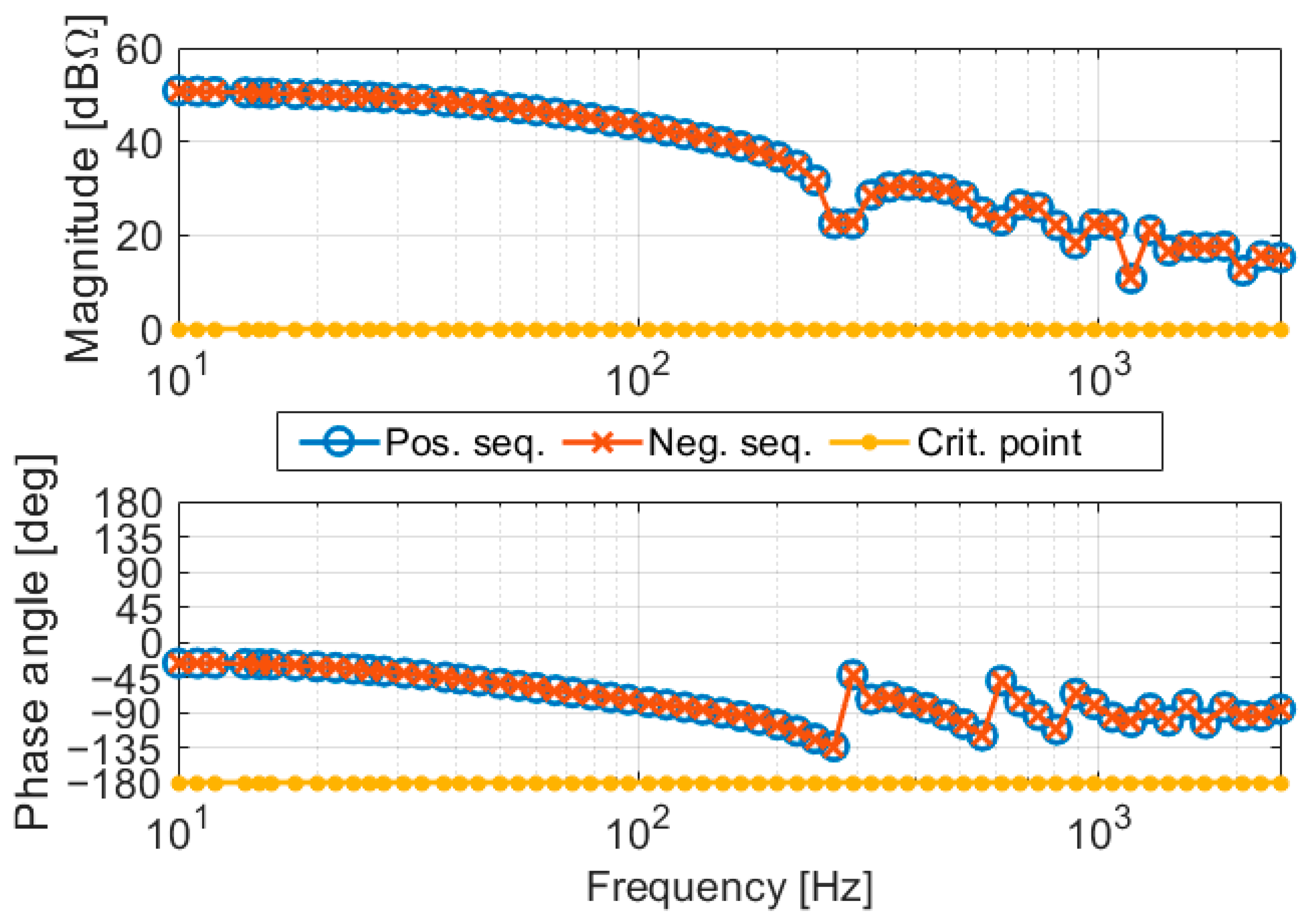
4. Frequency Domain Stability Analysis Method

The impedance-based stability criterion is a commonly used approach for conducting converter-driven stability analysis in the frequency domain [7]. This section provides a brief overview of the method, using a single converter–grid system, as depicted in Figure 3. A single-input single-output (SISO) converter-connected system can be modeled with voltage or current sources in series or parallel with a small-signal frequency-dependent impedance.

According to this approach, the stability of the converter–grid system is assessed by analyzing the small-signal frequency-dependent impedances of both the converter and the grid. This is performed using system theory tools such as the Nyquist criterion or Bode plots. According to this criterion, the system is stable when Equation (10) is satisfied.

$${\displaystyle \frac{\left|Z_N(f)\right|}{\left|Z_C(f)\right|}}=1andPM>0$$

(10)

$$PM=180°-\left[\arg \left(Z_N\left(f\right)\right)-\arg \left(Z_C\left(f\right)\right)\right]$$

(11)

The ratio of the network impedance to the converter impedance is also the loop gain of the SISO system shown in Figure 3. In other words, the condition defined by Equations (10) and (11) indicates that if the loop gain reaches 0 dB at a frequency $f$ and the phase margin (PM) is less than 0, the system is unstable. Generally, for the analysis of a SISO system, a Thevenin equivalent of the AC network or a frequency-dependent network equivalent is employed. However, as the number of converters integrated into the grid increases, a single network equivalent impedance becomes insufficient. Therefore, the stability analysis has to be carried out considering a multi-input multi-output (MIMO) system.

An investigation of various frequency-dependent stability analysis methods is conducted and presented in reference [10]. Based on the analysis, it was observed that the generalized nyquist criterion (GNC) is a robust method for conducting converter-driven stability analysis of a MIMO meshed network. Therefore, this method is utilized and further investigated for screening critical grid use cases. As mentioned in ref. [16], in the overall network, which is a MIMO system with multiple sources, as depicted in Figure 4, the nodal admittance matrix ($Y_{tot})$ can be expressed as the sum of the passive network admittance matrix ($Y_N)$ and the source admittance matrix ${(Y}_S$), represented by the following equations:

$$Y_{tot}=Y_N+Y_S$$

(12)

$$Y_S=\left(\begin{array}{ccc}{Y}_{C1}& \cdots & 0\\ ⋮& \ddots & ⋮\\ 0& \cdots & Y_{CN}\end{array}\right)$$

(13)

$Y_N$ is given by Equation (9), with the converter nodal admittances excluded. The loop gain for this system is then given by:

$$L=Z_N·Y_S$$

(14)

The eigenvalues of the loop gain are found by solving the following equation:

$$\det \left(L-\lambda ·I\right)=0$$

(15)

This results in a diagonal eigenvalue matrix, ${\lambda }_{n\times n}$, where $n$ represents the number of network buses. Finally, $n$ complex frequency-dependent eigenvalues are derived. Bode plots of these frequency-dependent eigenvalues are used for the stability analysis. According to the stability criterion and similar to Equation (10), if any of the eigenvalues reach 0 dB at frequency $f$ and have a phase margin (PM) lower than 0, the system is considered unstable.

For the screening of critical use cases, not only the grid use cases with a negative PM but also the grid use cases with a small positive PM are considered. For the frequency domain stability analysis, the system is linearized at a single operating point. That is, the effects of any switching events cannot be analyzed. Therefore, stability analysis in EMT tools is essential for grid use cases with smaller positive and negative phase margins. Nevertheless, the advantages of frequency domain impedance-based analysis cannot be ignored. In other words, the frequency-dependent impedance of the network is an important feature for understanding the stability. Therefore, owing to its advantages, these frequency-dependent impedances are utilized to determine the boundary buses necessary to conduct converter-driven stability analysis for any given network. Further, in the following section, the method to determine the boundary buses is discussed.

5. Frequency Domain Network Reduction Method

As stated in Section 3, the frequency-dependent admittance of each network component contributes to the final network admittance matrix. The strength of a node’s connection to the rest of the network is determined by its self-admittance, represented by the diagonal elements ($Y_{ii})$ of the admittance matrix and, equivalently, by $(Z_{ii})$ of its impedance matrix. This value reflects the total impedance associated with the node, including both self-connections (e.g., shunt/nodal components) and external connections (i.e., elements linking the node to other nodes in the network). From Section 4, it can be observed that network impedance characteristics at the point of common coupling play a significant role in analyzing the stability of the system.

Therefore, in this method, a sensitivity analysis is conducted by individually varying the admittance of each component proportional to its original value while keeping all the other admittances constant. The resulting change in the frequency-dependent network impedance at the converter’s connection point is then evaluated and is further compared with the original network impedance. Subsequently, the influence of each component on the network impedance is ranked. Based on the ranking, the boundary buses are identified, and the low-influence buses are reduced. Finally, the boundary buses are connected with power flow equivalents. The overview of the mathematical formulation for determining the boundary buses and further reducing the network size is described in a step-by-step methodology, as shown in Figure 5.

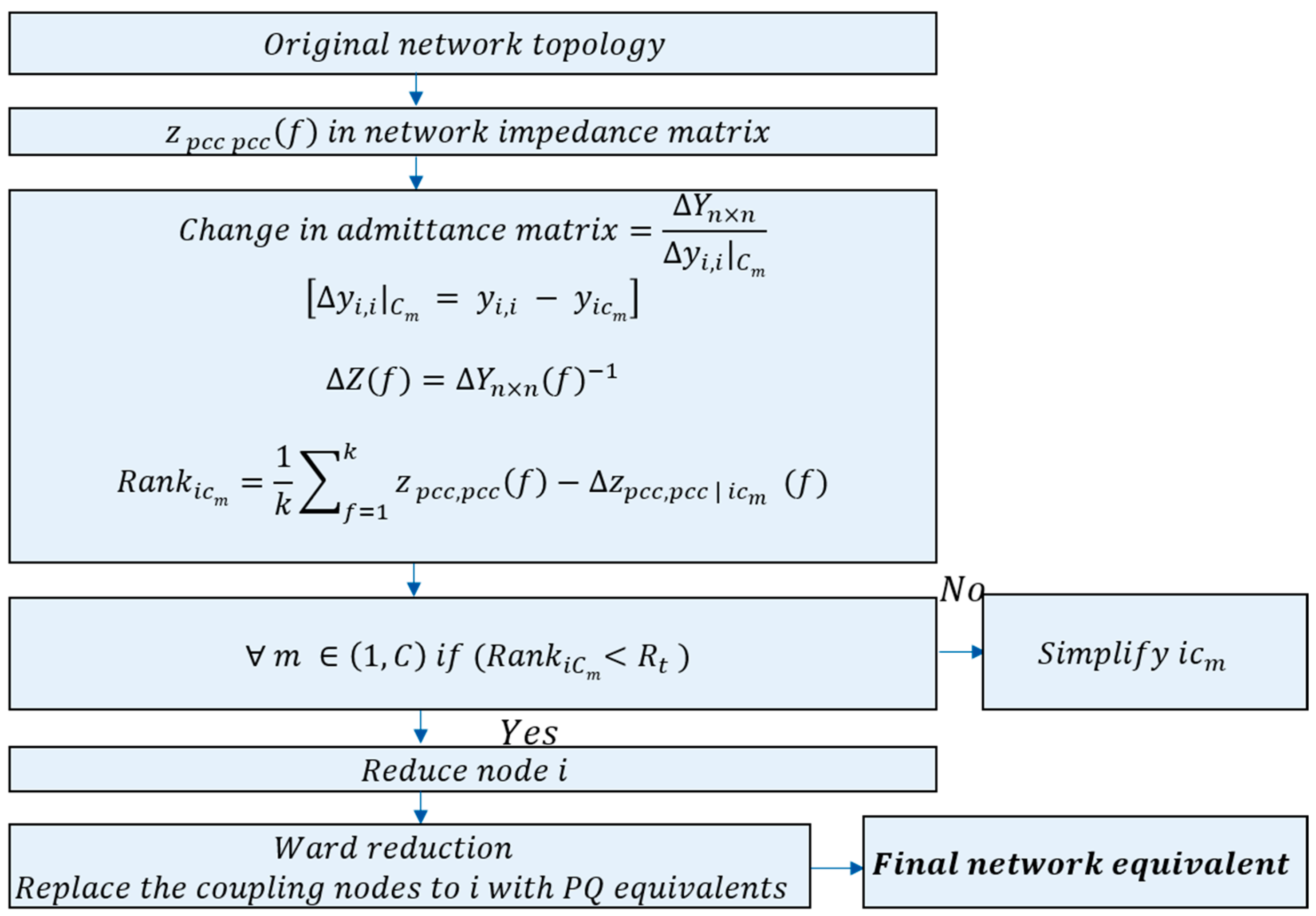
• Original network topology: The network topology is used to formulate the frequency-dependent admittance matrix of the network.
• Identification of original network impedance: The network impedance matrix is calculated using the formulated admittance matrix. The self-impedance (z_pcc,_pcc (f)) at the point of common connection (PCC) with the converter is identified.
• Sensitivity analysis: Sensitivity analysis is carried out by varying the admittance at a node proportional to the admittance of the components connected at the node. The following equation gives the change of the admittance at a node at one time.

  $$∆y_{i,i|C_m}=y_{i,i}-y_{i{c}_m}$$

  (16)

  where $c_m$ is the mth component connected at node $i$, $y_{i,i}$ is the original admittance of node $i,$ and $y_{i{c}_m}$ is the admittance of component $m$ at node $i$. For the change of admittance at a node, the change in the admittance matrix given by ${∆Y}_{n\times n}(f)$ is calculated. Here, $n$ is the number of buses in the original network topology.
• Identification of modified network impedance: The changed admittance matrix is inverted to obtain the modified impedance matrix ($∆Z(f)= \Delta Y_{n\times n}^{-1}(f))$. From this, the modified self-impedance (${∆z}_{pcc,pcc|{ic}_m}(f))$ is identified.
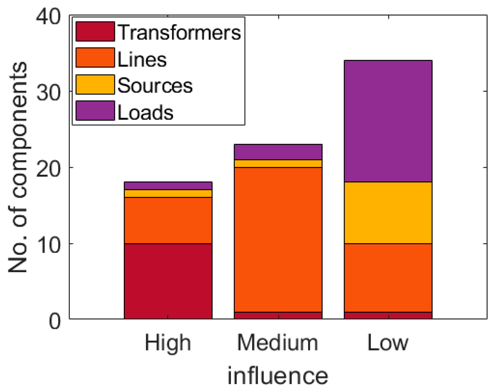
• Ranking metric: Using the modified self-impedance and the original self-impedance at PCC, the network components are ranked as low, medium, and high influence components. The ranking metric is given by the following equation.

  $${Rank}_{i{C}_m}={\displaystyle \frac{1}{k}}\sum _{f=1}^k(z_{pcc,pcc}\left(f\right)-∆z_{pcc,pcc|i{C}_m}\left(f\right))$$

  (17)
  It describes an average of the direct deviation of original and modified self-impedances over $k$ frequency set points.
• Node reduction condition: The buses are deemed low influence based on the ranking of the components at a bus. If all the components of a bus are of low rank, then the bus is eligible for reduction. However, if only a few components are of low influence, then the bus cannot be reduced, but the low-influence components of the bus can use simplified models. For example, if a transmission line is deemed low influence, the PI section models of the line, instead of wideband line models, can be used.
• Final network reduction: The boundary buses coupling the low-influence buses are identified. Through the ward reduction method, the low-influence buses are reduced, and the boundary buses are then connected to power flow equivalents. The resulting network has a smaller number of nodes but retains the power flow of the network and the frequency-dependent characteristics at the PCC.
• To summarize, this method uses the frequency-dependent impedances of the network calculated in stage one for obtaining component impedance sensitivities and for performing node reduction based on ranking metrics.

6. Results

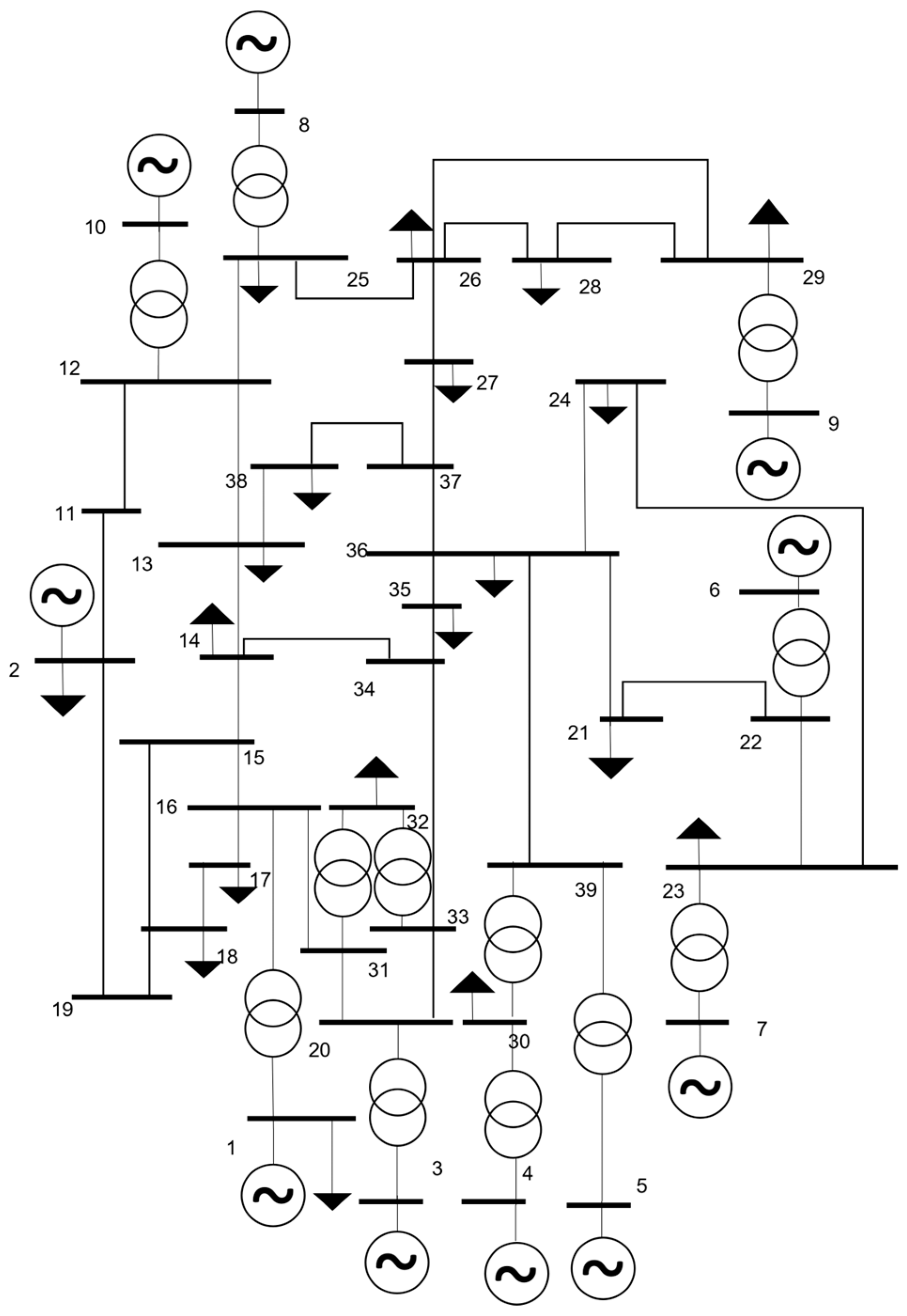
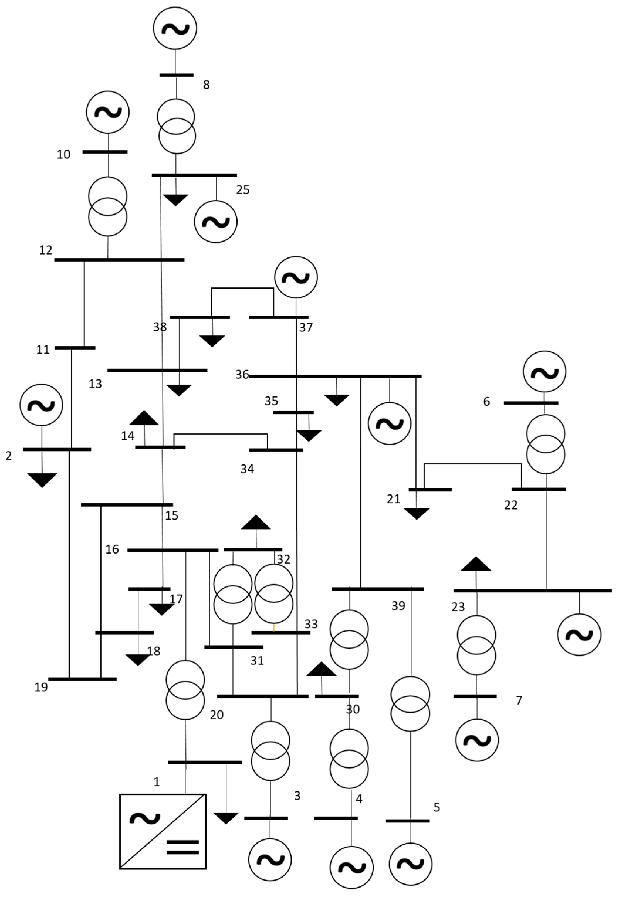
6.1. Test System and Use Case Definition

The generic test system utilized for this case study is an IEEE 39 bus system [17], though the grid parameters are modified to suit the in-house converter model. The network consists of 10 generators, 12 transformers, 19 loads, and 34 transmission lines. It operates at a voltage level of 220 kV and a system frequency of 50 Hz. The topology of the IEEE 39 bus system is shown in Figure 6.

Although the original grid use case consists of only generators, an additional grid use case is created by replacing the generator at bus 1 with a modular multilevel converter (MMC). Bus 1 is also considered as the PCC in the following study conducted. Therefore, the following use cases are tested:

• Use case 1: conventional generator at bus 1 (PCC) of the IEEE 39 bus system.
• Use case 2: MMC at bus 1 (PCC) of the IEEE 39 bus system.

As shown in Figure 7, the case study conducted validates the following three aspects obtained by the complexity reduction procedure using the EMT tool as a benchmark:

• Frequency-dependent network model
• Screening method or the frequency domain stability analysis method
• Frequency domain network reduction method

The EMT tool used in this study is HYPERSIM 2021.3.1.o187 from OPAL-RT Technologies.

6.2. Case Study

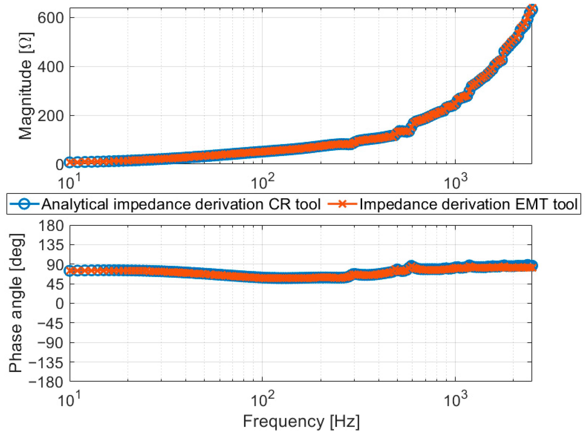
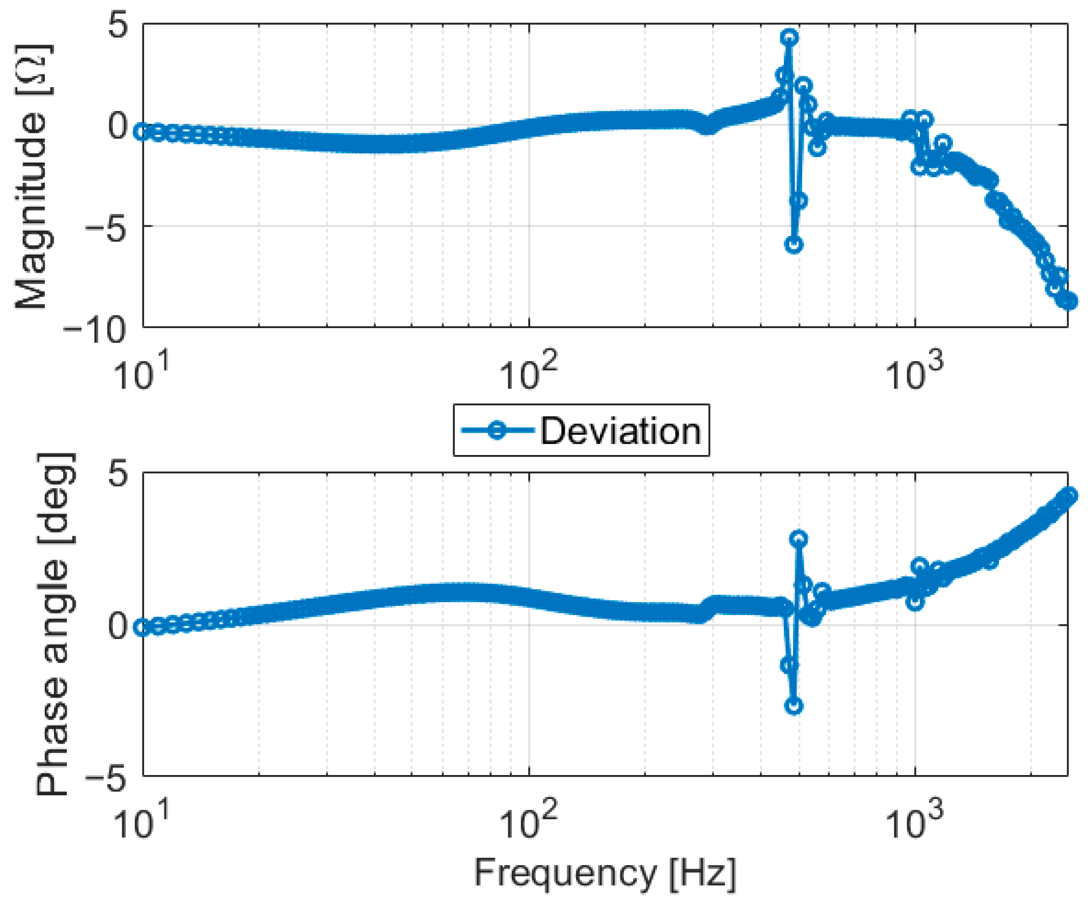
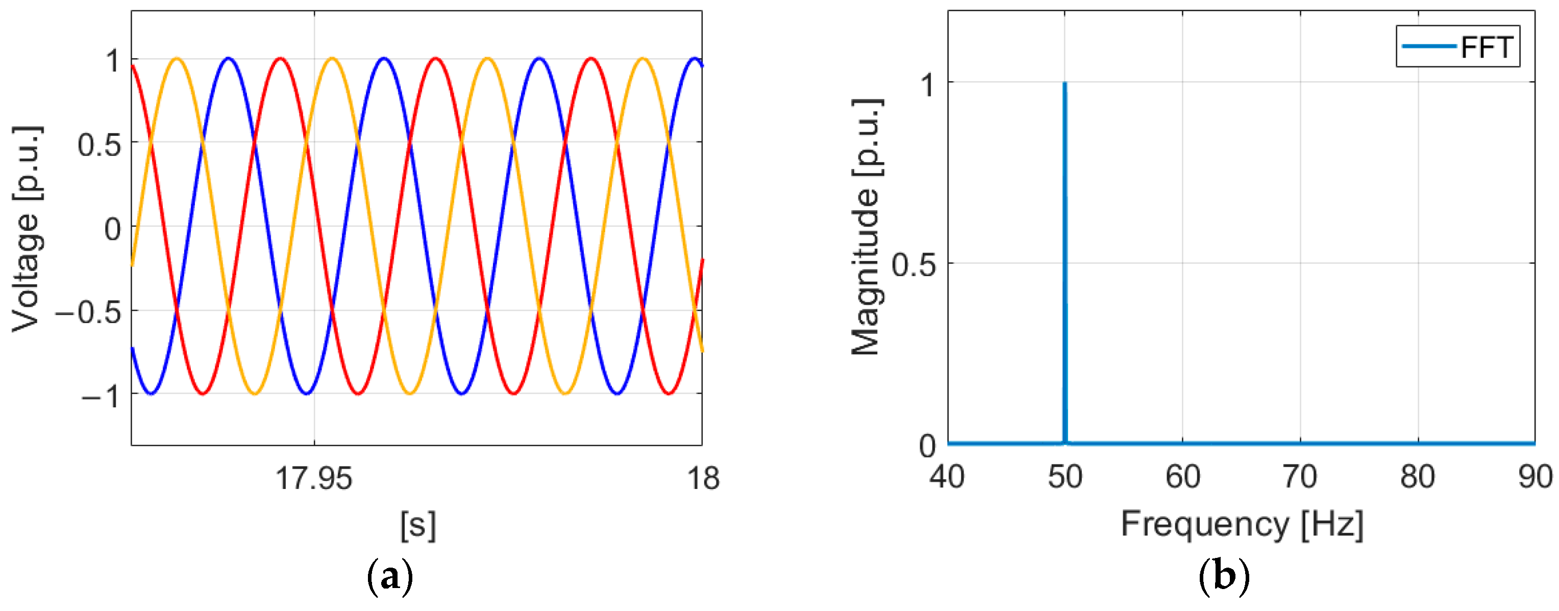
• Validation of Frequency Domain Network Model

Utilizing the data with respect to the network topology and component parameters, the IEEE 39 bus system is constructed as a frequency-dependent network impedance matrix within the tool. This network impedance matrix consists of frequency-dependent impedance at the PCC. The same network is constructed in the EMT tool using the detailed models available.

Using a sweeping method, as described in Section 3, the frequency-dependent impedance at the PCC is obtained from the EMT tool. The impedance obtained from both the complexity reduction (CR) procedure and the EMT tool is given in Figure 8. These impedances are compared, and their deviation is observed, as shown in Figure 9. It can be observed that the impedance magnitude and phase of the analytical impedance derived from the complexity reduction procedure and the impedance derived from the EMT tool show a deviation lower than 10 Ω and 5°, respectively. This is less than 1% of the direct deviation. Therefore, it can be concluded that the procedure accurately constructs the wideband models, i.e., frequency-dependent characteristics of the IEEE 39 bus system.

2.

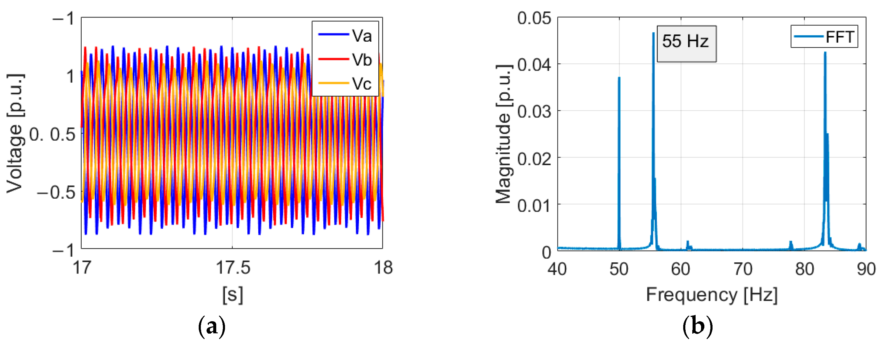
Validation of Frequency Domain Stability Analysis

Initially, the screening method is applied to use case 1, and the Bode criterion is analyzed. It is observed from the Bode plot shown in Figure 10 that no critical point exists where the stability margins are threatened. Therefore, the system is deemed stable, and use case 1 is not a critical use case. As this is the original network, these conclusions are to be expected. Nevertheless, it is presented here for comparison with the critical scenario.

Simulating use case 1 in the EMT tool results in a voltage waveform oscillating only at a system frequency of 50 Hz, as shown in Figure 11. This outcome aligns with expectations and is consistent with the conclusions drawn from the screening method.

Subsequently, the screening method is applied to use case 2, and the Bode plots are analyzed. From Figure 12, it can be observed from the Bode plot that at 55 Hz, the phase difference is close to 180° for the positive sequence plot and hence, the phase margin is close to zero. It can be concluded that the system, as defined for use case 2, may oscillate at 55 Hz in addition to 50 Hz system frequency. Simulating use case 2 in the EMT tool results in a voltage waveform oscillating at a frequency other than the system frequency. FFT analysis of the voltage waveform shows that 55 Hz is one of the frequencies at which the voltage signal oscillates, as predicted by the screening method, further showing that the screening method has rightly predicted the critical grid use case. The voltage waveform and its FFT analysis are shown in Figure 13.

3.

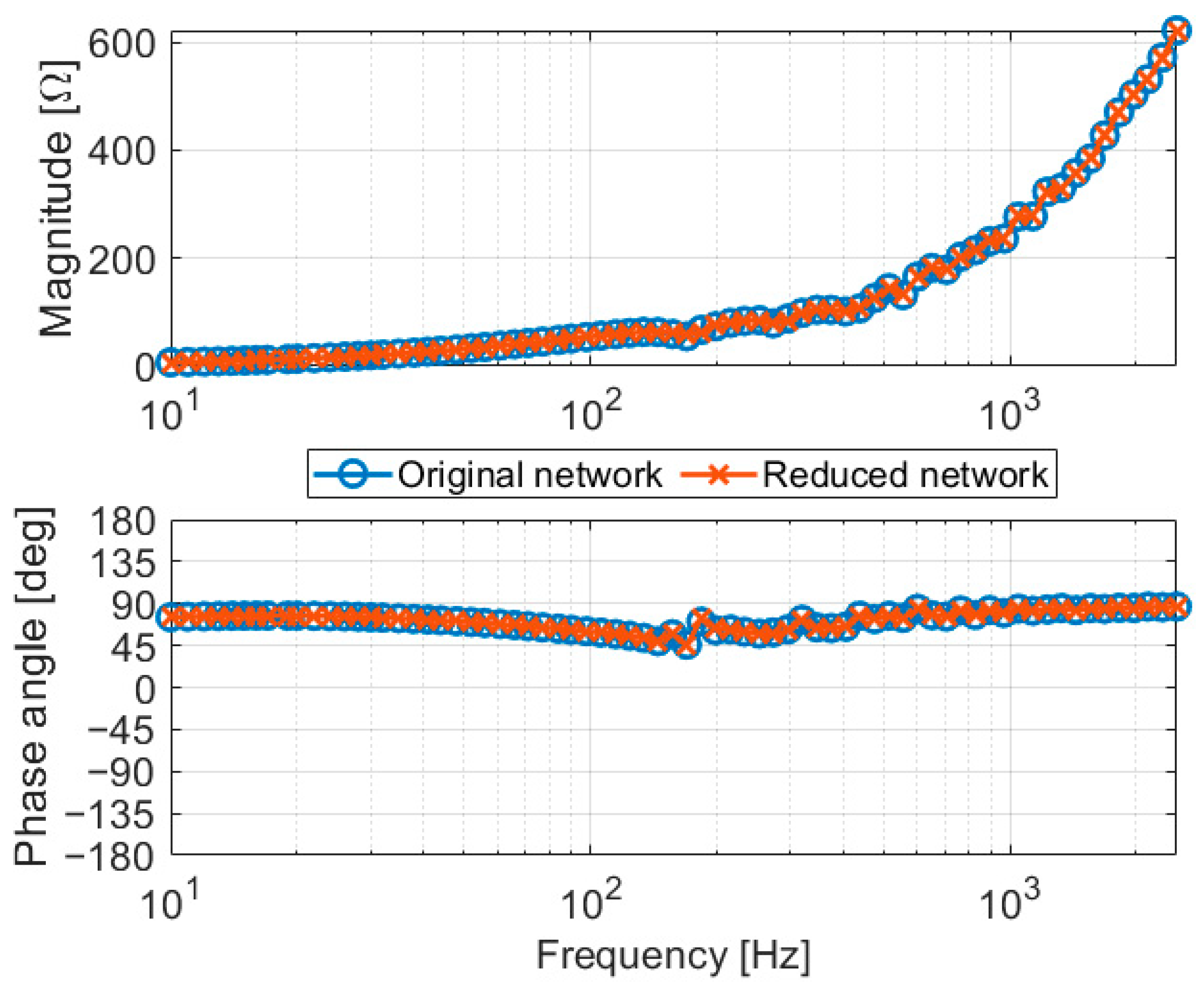
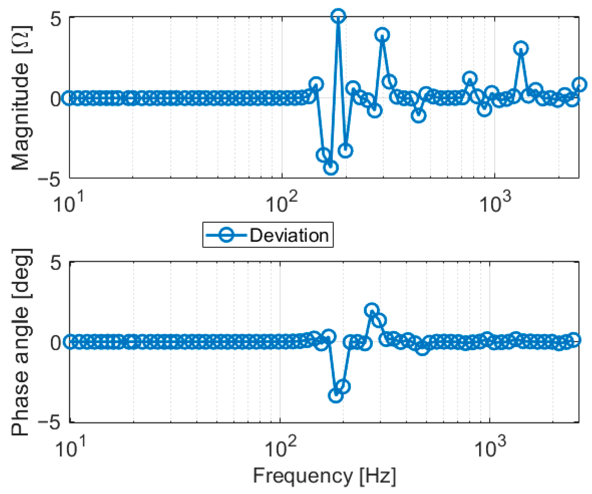
Validation of Frequency Domain Network Reduction Method

Use case 2, the critical use case as determined by the screening method, is given as an input to the network reduction method. Based on the procedure presented in Section 5, the impedance sensitivities are calculated, and based on the ranking metric, the network components are categorized as low, medium, and high influence components. The bar plot of the categorization is shown in Figure 14. If all the components connected to a bus are of low influence, then the bus is considered for network reduction. For this use case, after the application of the reduction method, buses 24, 26, 28, 27, 29, and 9 are in the low-influence region. Therefore, these six buses are reduced, and their coupling boundary buses are connected with power flow equivalents. It is observed that the influence does not necessarily depend on electrical distance. The final reduced network is shown in Figure 15.

The reduced network is further investigated to confirm its validity for performing converter-driven stability analysis in the EMT tool. For this, both in the frequency domain and time domain, the frequency-dependent characteristics at the PCC, as well as the oscillating frequency of the voltage waveform, are verified.

The impedance plots of the original and reduced network are given in Figure 16. From the analysis, it can be verified that the frequency-dependent characteristics of the reduced network show less than 1% deviations in comparison to the original network. The plots showing the direct deviation of these impedances are shown in Figure 17. It can also be observed that the analysis of the reduced network for the critical use case in the EMT tool shows that the system oscillates at the same 55 Hz frequency as in the original network, resulting in the same stability conclusions as those of the original network. The voltage plots and their corresponding FFT are shown in Figure 18. Additionally, it was observed that the total simulation run time of the reduced network is 12% faster than the original network for the execution of a single-use case.

It should be noted that the accuracy of the method largely depends on the frequency-dependent impedance models of the network and its components. The method has been tested and benchmarked with EMT tools over a frequency range of 10 Hz–2.5 kHz, for which it shows good accuracy. However, for the investigation of the interaction phenomena above this frequency range, further investigation into impedance modeling and analysis has to be considered.

7. Conclusions

In this paper, a complexity reduction procedure for converter-driven stability analysis in an EMT tool is introduced and applied to a generic test system. The procedure presented is a two-stage process, which is based on frequency domain modeling, analysis, and network reduction. The proposed procedure is applied to an IEEE 39 bus system, and the results are presented using two scenarios. As this is a frequency domain procedure, the EMT tool is used as a benchmark for validating the modeling and analysis that is carried out in the procedure. The case study presented outlines the accuracy of frequency domain modeling, analysis, and the validity of the proposed network reduction approach. The case study demonstrates that the frequency-domain modeling of the network and its components effectively captures the network’s frequency-dependent characteristics, similar to those represented by an EMT tool. Furthermore, the screening method utilized successfully predicts the critical grid use case. Finally, the procedure successfully reduces the network without compromising the quality of the stability analysis conclusions. In summary, the procedure lowers the number of grid use cases and the size of the network for analysis in the EMT tool. The presented method is investigated for analyzing interaction phenomena within the frequency range of 10 Hz to 2.5 kHz. Investigations outside this frequency range require further examination before applying the method.

References

1. Kundur, P. Power System Stability and Control; McGraw-HillP New York, NY, USA, 1993.
2. Hatziargyriou, N.; Milanovic, J.; Rahmann, C.; Ajjarapu, V.; Canizares, C.; Erlich, I.; Hill, D.; Hiskens, I.; Kamwa, I.; Pal, B.; et al. Definition and Classification of Power System Stability—Revisited & Extended. IEEE Trans. Power Syst. 2021, 36, 3271–3281. [Google Scholar] [CrossRef]
3. Buchhagen, C.; Rauscher, C.; Menze, A.; Jung, J. BorWin1—First Experiences with harmonic interactions in converter dominated grids. In Proceedings of the International ETG Congress 2015, Bonn, Germany, 17–18 November 2015. [Google Scholar]
4. CIGRE Study Committee C4. Electromagnetic Transient Simulation Models for Large-Scale System Impact Studies in Power Systems Having a High Penetration of Inverter-Connected Generation; C4 Technical Brochure Power System Technical Performance; CIGRE: Paris, France, 2022. [Google Scholar]
5. Lara, J.D.; Ramasubramanian, D. Revisiting Power Systems Time-domain Simulation Methods and Models. IEEE Trans. Power Syst. 2023, 38, 123–136. [Google Scholar]
6. Quester, M. Investigating Converter Control Interactions in the Transmission Grid; Fakultät für Elektrotechnik und Informationstechnik der Rheinisch-Westfälischen Technischen Hochschule Aachen: Aachen, Germany, 2021. [Google Scholar]
7. Sun, J. Impedance-Based Stability Criterion for Grid-Connected Inverters. IEEE Trans. Power Electron. 2011, 26, 3075–3078. [Google Scholar] [CrossRef]
8. Quester, M.; Yellisetti, V.; Puffer, F.L.R. Assessing the Impact of Offshore Wind Farm Grid Configuration on Harmonic Stability. In Proceedings of the 2019 IEEE Milan PowerTech, Milan, Italy, 23–27 June 2019; pp. 1–6. [Google Scholar] [CrossRef]
9. Zhang, M.M.A.R.; Cai, X.; Zhang, C.C. Impedance-based Analysis of Interconnected Power Electronics Systems: Impedance Network Modeling and Comparative Studies of Stability Criteria. IEEE J. Emerg. Sel. Top. Power Electron. 2020, 8, 881–894. [Google Scholar] [CrossRef]
10. Yellisetti, V.; El Azzati, O.; Moser, A. Investigation of Frequency Domain Analysis Methods for Converter-Driven Stability Evaluation of Converter-Dominated Meshed Systems. In Proceedings of the 2023 IEEE Belgrade PowerTech, Belgrade, Serbia, 25–29 June 2023; pp. 1–6. [Google Scholar] [CrossRef]
11. Salas, A.B. Control Interactions in Power Systems with Multiple VSC HVDC—Analysis, Modelling, and Mitigation. Ph.D. Dissertation, Arenberg Doctoral School, Faculty of Engineering Science, KU Leuven, Leuven, Belgium, 2018. [Google Scholar]
12. Technische Regeln für den Anschluss von Kundenanlagen an das Höchstspannungsnetz und Deren Betrieb (TAR Höchstspannung); VDE-AR-N 4130; VDE: Frankfurt, Germany, 2017.
13. Gatous, O.M.; Pissolato, J. Frequency-Dependent Skin-Effect Formulation for Resistance and Internal Inductance of a Solid Cylindrical Conductor. IEE Proc. Microw. Antennas Propag. 2004, 151, 212–216. [Google Scholar] [CrossRef]
14. CIGRE Joint Working Group C4/B4.38. Network Modelling for Harmonic Studies; CIGRE Technical Brochure No. 766; CIGRE: Paris, France, 2019. [Google Scholar]
15. Wedepohl, L.M.; Wilcox, D.J. Transient analysis of underground power-transmission systems—System model and wave propagation characteristics. Proc. Inst. Electr. Eng. 1973, 120, 253–260. [Google Scholar] [CrossRef]
16. Maciejowski, J.; Dagless, E. Multivariable Feedback Design. Electronic Systems; Addison-Wesley: Reading, MA, USA, 1989. [Google Scholar]
17. Hiskens, I. IEEE PES Task Force on Benchmark Systems for Stability Controls; IEEE: Piscataway, NJ, USA, 2013. [Google Scholar]
Figure 1. Workflow of the complexity reduction procedure.
Electronics 14 00055 g001
Figure 2. Setup for the numerical derivation of frequency-dependent converter impedance.
Electronics 14 00055 g002
Figure 3. Small-signal representation of a converter-connected SISO system.
Electronics 14 00055 g003
Figure 4. Multi-input multi-output system with n sources.
Electronics 14 00055 g004
Figure 5. Overview of the frequency domain network reduction method.
Electronics 14 00055 g005
Figure 6. IEEE 39 bus test system.
Electronics 14 00055 g006
Figure 7. Workflow for the case studies.
Electronics 14 00055 g007
Figure 8. Comparison of the frequency-dependent network impedance for use case 1 obtained from the complexity reduction procedure and the EMT tool.
Electronics 14 00055 g008
Figure 9. Direct deviation of the network impedance obtained from the complexity reduction procedure and EMT tool.
Electronics 14 00055 g009
Figure 10. Frequency domain stability analysis—use case 1.
Electronics 14 00055 g010
Figure 11. Validation of the frequency domain stability analysis in EMT tool—use case 1. (a) Voltage waveform. (b) FFT analysis of the voltage waveform.
Electronics 14 00055 g011
Figure 12. Frequency domain stability analysis—use case 2.
Electronics 14 00055 g012
Figure 13. Validation of the frequency domain stability analysis in EMT tool—use case 2. (a) Voltage waveform. (b) FFT analysis.
Electronics 14 00055 g013
Figure 14. Categorization of network components based on the ranking metric.
Electronics 14 00055 g014
Figure 15. Network after the application of the network reduction procedure.
Electronics 14 00055 g015
Figure 16. Comparison of the network impedance of the original network and the reduced network.
Electronics 14 00055 g016
Figure 17. Direct deviation of the network impedances of the original and reduced network.
Electronics 14 00055 g017
Figure 18. (a) EMT analysis and validation of the reduced network. (b) FFT of voltage at PCC.
Electronics 14 00055 g018
Disclaimer/Publisher’s Note: The statements, opinions and data contained in all publications are solely those of the individual author(s) and contributor(s) and not of MDPI and/or the editor(s). MDPI and/or the editor(s) disclaim responsibility for any injury to people or property resulting from any ideas, methods, instructions or products referred to in the content.