Research on INS/GNSS Integrated Navigation Algorithm for Autonomous Vehicles Based on Pseudo-Range Single Point Positioning

Abstract

This study proposes an enhanced integration framework for the global navigation satellite system (GNSS) and inertial navigation system (INS). The framework combines real-time differential GNSS corrections with an adaptive extended Kalman filter (EKF) to address positional accuracy and system robustness challenges in practical navigation scenarios. The proposed method dynamically compensates for positioning inaccuracies and sensor drift by integrating differential GNSS corrections to reduce errors and employing an adaptive EKF to address temporal synchronization discrepancies and misalignment angle deviations. Simulation and experimental results demonstrate that the framework keeps horizontal positioning error within 2 m and achieves a maximum accuracy improvement of 4.2 m compared to conventional single-point positioning. This low-cost solution ensures robust performance for practical autonomous navigation scenarios.

1. Introduction

High-precision localization is crucial for autonomous vehicles, robotics, and geospatial applications [1]. Within the technical framework of autonomous vehicles, perception, decision-making, and control technologies form the core structure. Among these, high-precision positioning plays a pivotal role, directly influencing safe navigation, vehicle trajectory tracking, and lane changing. As a critical component, the effectiveness of path-following control is heavily dependent on the accuracy of the onboard positioning system [2]. In recent years, GNSS/INS integration has gained significant attention as a promising approach to overcoming the limitations of standalone GNSS in complex environments. Therefore, the demand for precise vehicle localization has become a critical factor in ensuring both safety and efficiency in autonomous navigation.

The global navigation satellite system (GNSS) and inertial navigation system (INS) are extensively used in real-time positioning due to their complementary capabilities. GNSS offers absolute positioning accuracy under open-sky conditions, but it is susceptible to positioning errors caused by environmental factors and hardware limitations. INS, in contrast, operates independently of external signals, providing high-rate motion estimation. However, it suffers from long-term cumulative errors, which can degrade positioning accuracy over time. The integration of GNSS and INS has been extensively studied, with various fusion techniques being explored to optimize positioning accuracy and robustness [3].

This study introduces a GNSS/INS integration framework designed for practical navigation scenarios where positioning performance may be affected by common interference factors. By incorporating real-time differential GNSS corrections and an adaptive extended Kalman filter (EKF), the proposed method dynamically reduces positioning errors and mitigates inertial sensor error accumulation. The EKF optimizes error state estimation by addressing misalignment angles, time synchronization offsets, and sensor drift. This approach ensures robust autonomous navigation in various practical environments, achieving meter-level positioning accuracy under typical operating conditions. The framework’s scalability and reliability are demonstrated through systematic error modeling and adaptive compensation strategies, significantly enhancing the robustness and precision of the navigation system in real-world applications.

High-precision localization is crucial for autonomous vehicles’ practical applications, where GNSS performance may be suboptimal. RTK (real-time kinematic) and PPP (precise point positioning) are superior in terms of accuracy: RTK can achieve centimeter-level positioning under ideal conditions with continuous base station corrections, while PPP enables decimeter-level accuracy after a sufficient convergence period. However, their widespread application in cost-sensitive autonomous vehicles is hindered by practical constraints.

In contrast, single-point positioning (SPP) was strategically adopted owing to its minimal hardware requirements, ultra-low computational overhead, and complete independence from external base-station infrastructure, all of which render it particularly suitable for mass-produced autonomous vehicles with stringent cost constraints.

Field experiments demonstrate that the proposed method reduces the maximum positioning error by 4.2 m, achieving horizontal accuracy better than 2 m. This level of precision is sufficient for core autonomous driving tasks such as trajectory tracking. Notably, these results are achieved without the additional hardware, continuous correction services, or extended convergence times typically required by RTK or PPP, making SPP-based integration a pragmatic choice for real-world autonomous vehicle applications.

2. Related Works

GNSS/INS integration has been extensively studied to enhance positioning accuracy and system robustness in various navigation applications. Based on different levels of interaction between GNSS and INS subsystems, early studies classified the integration into loosely, tightly, and ultra-tightly coupled architectures [4]. Boguslawski et al. [4] provided a comprehensive review of these approaches for land and aerial vehicles, highlighting key challenges such as lever-arm effects and sensor synchronization errors. However, traditional coupling schemes often suffer from error accumulation due to IMU drift over time.

To address these limitations, researchers have explored adaptive filtering and multi-sensor fusion strategies. Guo et al. [5] integrated 5G signals with adaptive step-size Kalman filtering, demonstrating improved positioning accuracy while maintaining computational efficiency. Karlgaard et al. [6] demonstrated improved accuracy in dynamic operational environments, though systems remain vulnerable to error accumulation and sensor drift. Wang et al. [7] introduced tightly coupled GPS/INS integration using optimized Kalman filters, whereas Zhang et al. [8] applied deep neural networks to compensate for INS errors. While these methods achieved enhanced accuracy, they typically require expensive hardware components and substantial computational resources.

Adaptive filtering techniques have also gained attention for their ability to adjust noise covariance in real-time. Wei et al. [9] proposed adaptive algorithms to improve error estimation in specific scenarios, while Ge et al. [10] developed a robust adaptive EKF with dual-window Sage-Husa estimation, achieving higher positioning accuracy in challenging environments. He et al. [11] classified GNSS/INS integrated navigation into four models (ultra-tightly/tightly/semi-tightly/loosely coupled), comparing their advantages and disadvantages. These findings underscore the need for adaptive frameworks that dynamically align noise covariance with operational conditions. These methods effectively mitigate some drawbacks of fixed-parameter filters but still face challenges in terms of cost and implementation complexity.

Hybrid approaches combining signal processing and machine learning have shown promising results. Li et al. [12] proposed an EMD-IMM-EKF-ELM framework for low-cost GPS/INS systems, reducing positioning errors during signal interruptions. Similarly, Wu et al. [13] introduced a failure-resistant tightly coupled GNSS/INS/vision system that maintains sub-meter accuracy in urban environments. Singh et al. [14] integrated deep learning with traditional filters using spatiotemporal attention networks for urban localization. Li et al. [15] proposed a graph-optimized GNSS/INS system with a reliability factor for real-time fault detection. Dai et al. [16] further explored the use of deep learning and recurrent neural networks to enhance positioning robustness. Li et al. [12] proposed a similar hybrid approach (EMD-IMM-EKF-ELM) for GPS outages. Amami [17] highlighted limitations of low-cost single-frequency systems, including multipath susceptibility. Despite these innovations, computational complexity hinders scalability [18]. Emerging approaches like factor graph optimization [19] and DS-SVM hybrid algorithms [12] demonstrate enhanced robustness but face cost-sensitivity challenges.

At the system level, several innovations have focused on improving reliability and integrity. Chen et al. [20] proposed adaptive Kalman filtering with outlier detection, reducing positioning errors by 35%. The noise-adaptive fusion framework by the Army Academy [21] introduced dual noise estimation models, achieving a 36.7% reduction in trajectory errors under intermittent GNSS conditions. Al Hage et al. [22] emphasized localization integrity through fault detection, while Zhu et al. [23] established PPP models for smartphone-based GNSS receivers. Kim et al. [24] reviewed multi-sensor fusion in GNSS-denied environments. Yurtsever et al. [25] surveyed autonomous driving technologies. Wang et al. [26] demonstrated differential positioning in dynamic scenarios, while Zhu et al. [23] validated signal processing for multipath mitigation. These reinforce experimental validation’s importance. Despite these contributions, existing methods still require improvement in terms of cost-effectiveness and accuracy enhancement [27].

Recent efforts have also been directed toward integrating advanced control strategies and optimization techniques. Liang et al. [28] proposed a polytopic-model-based robust model predictive control scheme with non-parallel distributed compensation and robust disturbance rejection to achieve accurate and reliable path tracking for autonomous vehicles under time-varying velocity and disturbances. Li et al. [29] proposed multi-sensor fusion for urban localization. Chen et al. [30] validated differential positioning for GPS accuracy. Liu et al. [31] implemented edge computing for differential corrections. Abdelmoniem et al. [32] presented predictive path-tracking controllers. Liang et al. [33] introduced velocity-based path-following control for friction management. To address limitations, recent studies focus on system synergy. Liang et al. [34] proposed a unified deep-reinforcement-learning framework that jointly optimizes behavioral decision-making, path planning, and model-predictive motion control to enable safe, human-like, and high-speed cruising of autonomous vehicles in mixed-traffic environments. Liang et al. [35] developed model-free path-following control. Although these approaches offer enhanced functionalities, they typically demand high-performance computing resources and extensive environmental modeling, which contradicts the objective of low-cost navigation systems.

Overall, although significant progress has been made in GNSS/INS integration, there remains a critical need for a low-cost yet high-accuracy solution. Existing methods either incur excessive costs or fall short in accuracy, particularly when employing consumer-grade sensors. This motivates our work to propose a novel differential GNSS/INS integration framework that effectively mitigates GNSS positioning uncertainties and INS error accumulation through adaptive EKF, achieving high precision while significantly reducing system costs.

This paper evaluates the system through real-road tests. The main contributions of this paper are stated as follows.

(1)

The proposed integrated GNSS/INS navigation framework achieves reliable positioning performance at low cost by fusing real-time differential GNSS corrections with an adaptive EKF, enhancing the stability of vehicle localization through three key mechanisms. Leveraging low-cost off-the-shelf components (e.g., ATK1218-BD GNSS module and MPU6050 IMU), it effectively reduces IMU error accumulation and improves GNSS positioning accuracy via adaptive error compensation. Specifically, the EKF addresses misalignment angle errors by rapidly dampening fluctuations in pitch, roll, and heading angles. The integration of differential GNSS plays a key role in mitigating GNSS positioning errors caused by common environmental interferences in typical scenarios, thereby reducing error accumulation, while the EKF optimizes velocity error management, with oscillations in eastward and northward directions controlled and converging quickly.

(2)

The experimental outcomes indicate that the integrated navigation system maintains a navigation accuracy within a 2-m range, exhibiting robust tracking performance. Outdoor tests showed a significant enhancement in positioning accuracy, with velocity errors controlled within ±0.15 m/s and heading angle errors within ±0.14°. The improvement in positioning accuracy was approximately 4.2 m. These results confirm the effectiveness of the position differential technique in enhancing positioning accuracy under practical operating conditions.

3. Positioning System Model

3.1. Differential GNSS Positioning System

Traditional GNSS/INS integration methods often suffer from sensor drift and positioning errors. To address these limitations, this study proposes a novel framework that integrates real-time differential GNSS corrections with an adaptive EKF. The differential GNSS corrections reduce positioning errors from common interference sources, while the EKF dynamically compensates for inertial sensor error accumulation and residual inaccuracies. By jointly addressing misalignment angles, time synchronization discrepancies, and sensor drift, the EKF optimizes error state estimation. Experimental results show that the framework achieves enhanced positioning accuracy and system stability in practical navigation scenarios.

Pseudo-range positioning relies on precise time synchronization between satellites and receivers. However, due to hardware limitations, the satellite clock bias ($\delta t_s$) and receiver clock bias ($\delta t_r$) introduce errors in the measured pseudo-range. These errors, along with ionospheric and tropospheric delays, need to be accounted for to improve positioning accuracy.

Figure 1 illustrates the relationship between GNSS time, satellite time, and receiver time, demonstrating how these biases affect the computed pseudo-range.

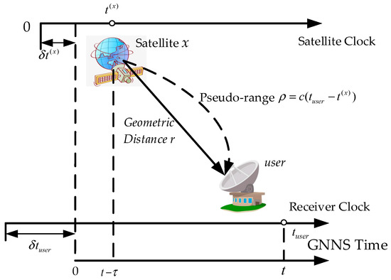
Figure 1. Pseudo-range, satellite clock error, and receiver clock error.

The pseudo-range equation can be expressed as:

$$P^{(n)}=p^{(n)}+\delta t_r-E^{(n)}-T^{(n)}$$

(1)

where $P^{(n)}$ represents the corrected pseudo-range, $p^{(n)}$ is the observed pseudo-range, $\delta t_r$ is the receiver clock bias, $E^{(n)}$ and $T^{(n)}$ are the ionospheric and tropospheric delays, respectively.

Given at least four visible satellites, the receiver’s position and clock offset can be estimated by solving the following pseudo-range equation:

$$P_r={\left({(x^{(n)}-x)}^2+{(y^{(n)}-y)}^2+{(z^{(n)}-z)}^2\right)}^{1/2}$$

(2)

where $(x,y,z)$ represents the receiver’s position, and $(x^{(n)},y^{(n)},z^{(n)})$ denotes the known coordinates of satellite $n$. However, the computed pseudo-range is affected by multiple error sources, including satellite clock bias, receiver clock bias, ionospheric delay, and tropospheric delay.

To improve positioning accuracy, these errors must be estimated and mitigated. The ionospheric and tropospheric delays introduce signal propagation errors, while satellite and receiver clock biases result in systematic timing deviations. The combined effect of these errors can be minimized using appropriate correction models.

Positioning errors can be categorized into two types: systematic biases and random noise. Systematic biases originate from predictable sources, such as satellite clock drift and atmospheric effects, whereas random noise results from unpredictable signal disturbances. To enhance positioning accuracy, this study employs Differential GNSS (DGNSS), which is an effective method for error mitigation.

DGNSS relies on a reference station with a precisely known location, which continuously records GNSS signal deviations and transmits real-time corrections to mobile receivers. With these corrections applied, systematic errors such as satellite clock bias and atmospheric delays are significantly reduced, enabling more accurate positioning, particularly in high-precision navigation applications.

SPP was selected for this study due to its minimal hardware requirements, making it highly suitable for cost-sensitive autonomous vehicle applications. Unlike RTK, which relies on base stations with substantial infrastructure costs, and PPP, which necessitates over 30 min for convergence, SPP operates independently and provides real-time updates. This characteristic renders SPP particularly pragmatic for navigation purposes.

Regarding the differential corrections, the differential correction amount at the GNSS receiver on the base station is as follows:

$$\left\{\begin{array}{c}\Delta x=x_R-x_B\\ \Delta y=y_R-y_B\\ \Delta z=z_R-z_B\end{array}\right.$$

(3)

where $x_R$, $y_R$, $z_R$ represent the precise reference coordinates of the base station GNSS; $x_B$, $y_B$, $z_B$ are the received coordinates of the base station GNSS.

The mobile station GNSS can obtain the above correction terms through communication and correct its own coordinates, thus having

$$\left\{\begin{array}{c}{x}_{M^{\prime }}=x_M+\Delta x\\ y_{M^{\prime }}=y_M+\Delta y\\ z_{M^{\prime }}=z_M+\Delta z\end{array}\right.$$

(4)

where $x_M$, $y_M$, $z_M$ are the received coordinates of the mobile station GNSS; $x_{M\prime }$, $y_{M\prime }$, $z_{M\prime }$ are the corrected coordinate values.

Considering the system’s data processing capabilities and communication delays, the mobile station GNSS receiver needs to perform delay compensation when applying the correction information:

$$\left\{\begin{array}{c}{x}_{M^{\prime }}=x_M+\Delta x+{\displaystyle \frac{d\Delta x}{dt}}(t_M-t_B)\\ y_{M^{\prime }}=y_M+\Delta y+{\displaystyle \frac{d\Delta y}{dt}}(t_M-t_B)\\ z_{M^{\prime }}=z_M+\Delta z+{\displaystyle \frac{d\Delta z}{dt}}(t_M-t_B)\end{array}\right.$$

(5)

where $t_M$ represents the current UTC time of the mobile station GNSS receiver, and $t_B$ represents the moment when the base station transmitted the information.

3.2. Inertial Navigation System Algorithms and Mechanical Arrangement

The strapdown inertial navigation system (SINS) is the core of integrated navigation, autonomously measuring the carrier’s attitude, angular velocity, and linear acceleration through built-in gyroscopes and accelerometers. Although the SINS does not rely on external signals, errors accumulate over time, affecting the accuracy of long-term navigation. To improve reliability, integrated navigation technology fuses SINS with GNSS data to correct SINS errors and ensure navigation accuracy.

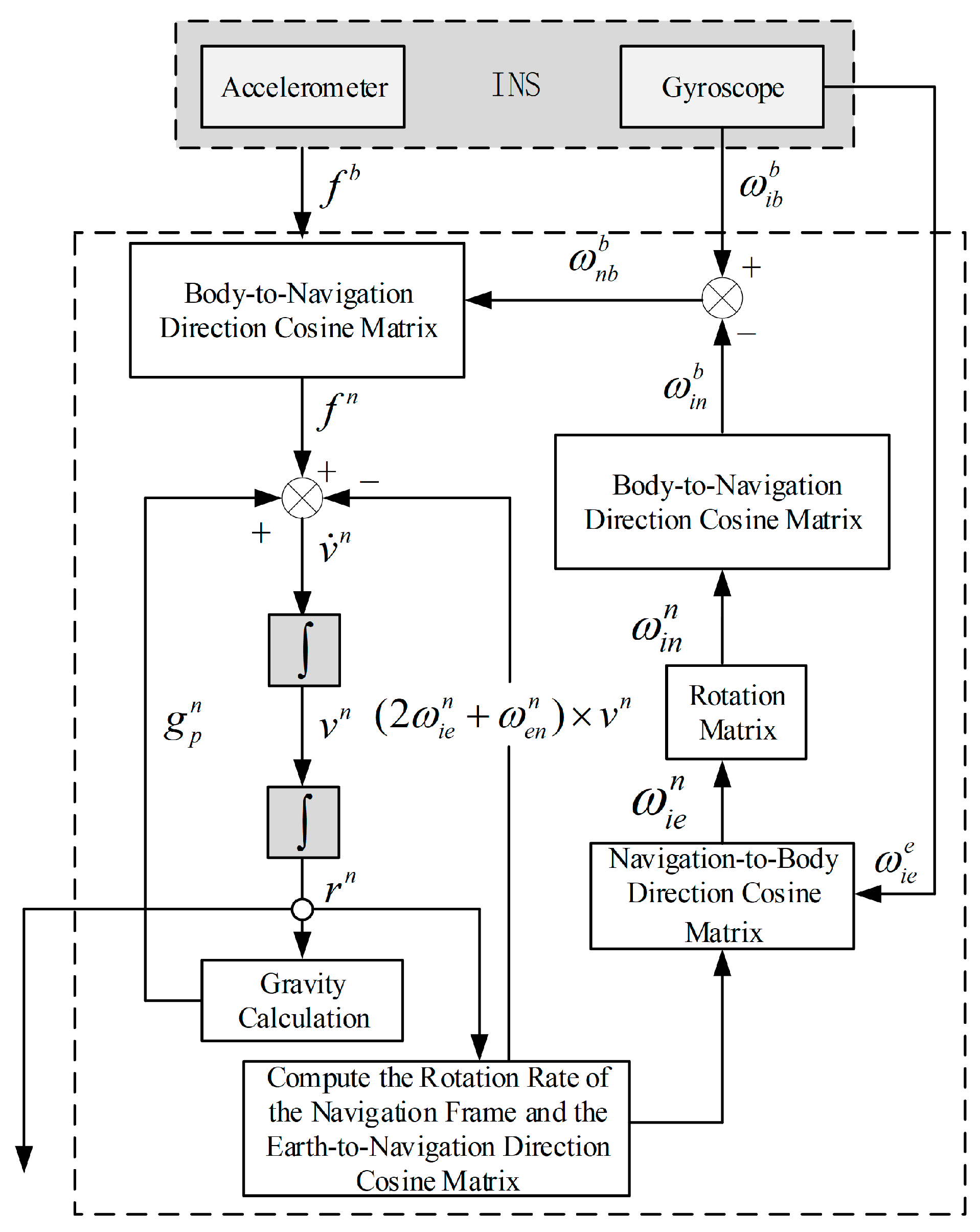
In SINS, the mechanical arrangement is a key process for obtaining carrier motion information. Accelerometers first measure the carrier’s specific forces, which are then transformed from the carrier coordinate system to the navigation coordinate system using the attitude matrix. The calculation of the attitude matrix depends on the attitude angles measured by the gyroscopes. After the specific forces are converted to the navigation coordinate system, the effects of Coriolis acceleration and local gravitational acceleration must be removed to obtain the motion acceleration free of harmful influences.

The mechanical arrangement process includes receiving data from the INS’s accelerometers and gyroscopes, transforming specific forces from the body coordinate system to the navigation coordinate system using the direction cosine matrix, calculating the rotation matrix, and obtaining acceleration in the navigation coordinate system. Subsequently, using the direction cosine matrix from the navigation coordinate system to the body coordinate system, the gravitational acceleration is calculated, and further calculations are made for the navigation coordinate system’s rotation rate and the direction cosine matrix from the Earth coordinate system to the navigation coordinate system. This process ensures the accurate acquisition of carrier motion information, providing key data support for the integrated navigation system.

The mechanical arrangement process is as follows (Figure 2):

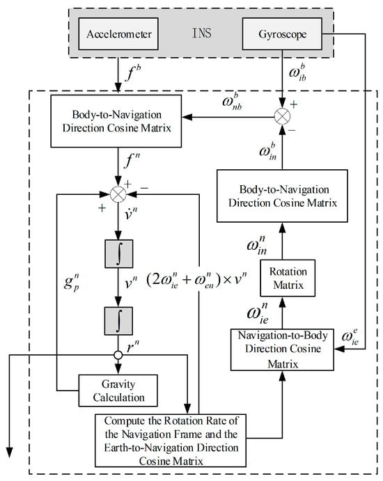
Figure 2. Strapdown inertial navigation mechanical arrangement.

The attitude solution algorithm can be expressed as follows:

$${\omega }_{in}^n={\omega }_{ie}^n+{\omega }_{en}^n$$

(6)

with

$${\omega }_{ie}^n={\left[\begin{array}{ccc}0& {\omega }_{ie}\cos L& {\omega }_{ie}\sin L\end{array}\right]}^T$$

(7)

$${\omega }_{en}^n={\left[\begin{array}{ccc}-{\displaystyle \frac{v_N}{R_M+h}}& {\displaystyle \frac{v_E}{R_N+h}}& {\displaystyle \frac{v_E}{R_N+h}}\tan L\end{array}\right]}^T$$

(8)

where ${\omega }_{ie}$ represents the Earth’s rotation angular velocity; $L$, $h$ are the local latitude and altitude; $v_N$, $v_E$ are the velocities in the navigation coordinate system along the northward and eastward directions, respectively; $R_M$, $R_N$ are the radii of curvature of the prime vertical and meridian circles at that latitude.

The differential equation of velocity in inertial navigation can be expressed as follows:

$${\dot{v}}^n=C_b^n{f}_{sf}^b-(2{\omega }_{ie}^n+{\omega }_{en}^n)\times v^n+g^n$$

(9)

where $v^n$ represents the vehicle’s ground velocity; $f^n$ is the specific force measurement value; $g^n$ is the local gravitational acceleration, which can be written as follows:

$$v^n={\left[\begin{array}{ccc}{v}_N& v_E& v_D\end{array}\right]}^T$$

(10)

$$f_{sf}^b={\left[\begin{array}{ccc}{f}_x^b& f_y^b& f_z^b\end{array}\right]}^T$$

(11)

The position information obtained by inertial navigation is actually obtained by integrating velocity, and the position’s longitude, latitude, and altitude information can be represented by the following equations:

$$\left\{\begin{array}{l}\dot{L}=1/(R_M+h)v_N\hfill \\ \dot{\lambda }=\sec L/(R_N+h)v_E\hfill \\ \dot{h}=v_U\hfill \end{array}\right.$$

(12)

with

$$R_M={\displaystyle \frac{R_N(1-e^2)}{(1-e^2{\sin }^{2}L)}}$$

(13)

$$R_N={\displaystyle \frac{R_e}{{(1-e^2{\sin }^{2}L)}^{1/2}}}$$

(14)

$$e=\sqrt{2f-f^2}$$

(15)

Thus, by integrating the mechanical arrangement of SINS, the output of inertial navigation can be obtained.

During the integrated navigation process, the imprecision of initialization and the accumulation of systematic errors can affect navigation performance. To improve navigation accuracy, it is necessary to establish an error model and perform compensation. Installation errors of gyroscopes and accelerometers can lead to discrepancies between measured data and true values. These discrepancies need to be quantified and compensated for through an error model.

The gyroscope measurement error can be expressed as follows:

$$\delta w_b^h=\delta K_C{\dot{\alpha }}_b^h+s^h$$

(16)

where $\delta w_b^h$ is the measurement error of the gyroscope, $\delta K_C$ is the scale factor error matrix of the gyroscope, and $s^h$ is the bias error.

The measurement error model for the accelerometer is as folows:

$$\delta f_a^b=\delta K_A{f}_a^b+{\nabla }^b$$

(17)

where $\delta f_b^h$ is the measurement error of the accelerometer, $\delta K_A$ is the scale factor error matrix of the accelerometer, and ${\nabla }^b$ is the measurement bias. By establishing an error model, compensation can be made for the measured data, thereby improving the accuracy of the navigation system. The key to error compensation lies in accurately estimating and correcting the measurement errors of the gyroscope and accelerometer.

3.3. Inertial Navigation Output Error Modeling and Initial Alignment

Accurate navigation in autonomous vehicles relies on precise state estimation, yet conventional GNSS+IMU systems face inherent challenges. GNSS measurements are vulnerable to systematic errors such as satellite clock bias, ionospheric and tropospheric delays, and multipath effects, particularly in complex environments. Meanwhile, standalone INS is prone to error accumulation, drift, and bias, which, if left uncorrected, can lead to significant deviations over time. To overcome these limitations, our integrated approach focuses on establishing a comprehensive error model and performing accurate initial alignment.

In our method, we develop an error state model that incorporates key INS error sources, including the measurement errors of gyroscopes and accelerometers, lever-arm discrepancies between the GNSS and IMU sensors, and time synchronization mismatches. This model forms the basis for the extended state Kalman filter (EKF) used in our data fusion process. By modeling the attitude, velocity, and position errors, our system effectively compensates for the INS drift, thereby enhancing overall navigation accuracy.

The primary sources of inertial measurement errors are the gyroscopes and accelerometers, which respectively measure angular velocity and acceleration. In practical applications, sensor readings typically contain scale factor errors, bias errors, and random noise. The angular velocity measured by a gyroscope can be expressed as follows:

$${\omega }_b^m={(C_b^n)}^T\{(I-diag(\delta k_g)){\omega }_b^t-{\epsilon }^g\}$$

(18)

where ${\omega }_b^m$ is the measured angular velocity, ${\omega }_b^t$ is the true angular velocity, $\delta k_g$ represents the scale factor error, and ${\epsilon }^g$ denotes gyroscope noise. Similarly, the measurement error model for an accelerometer is given by the following:

$$f_b^m=(I-diag(\delta k_a))f_b^t-{\epsilon }^a$$

(19)

where $f_b^m$ is the measured acceleration, $f_b^t$ is the true acceleration, $\delta k_a$ represents the scale factor error, and ${\epsilon }^a$ denotes accelerometer noise. It is evident that inertial measurement errors affect the accuracy of attitude, velocity, and position calculations. Consequently, establishing appropriate error propagation equations is necessary to analyze the impact of these errors systematically.

First, the attitude error equation describes the evolution of attitude errors over time. Under the small-error assumption, attitude errors propagate through the gyroscope measurement errors, and their differential equation is expressed as follows:

$$\dot{\varphi }=(I-\delta k_g)({\omega }_b^t-{\omega }_b^m)-{\epsilon }^g$$

(20)

where $\varphi$ represents the attitude error vector. This error primarily arises from gyroscope scale factor errors, noise, and true angular velocity errors. Since attitude errors directly influence navigation solutions and subsequently affect velocity and position calculations, their modeling and compensation are crucial in inertial navigation error analysis.

Next, the velocity error equation characterizes the cumulative effect of velocity errors over time. Given that accelerometer measurement errors directly affect velocity calculations, the velocity error can be obtained by integrating the acceleration error, expressed as follows:

$$\delta v^n={\displaystyle \int [(I-\delta k_a)f_b^t-f_b^m-{\epsilon }^a]}\mathrm{dt}$$

(21)

where $\delta v^n$ represents the velocity error. This error is influenced not only by accelerometer scale factor errors and noise but also indirectly by inertial system attitude errors and gyroscope errors. Due to the cumulative nature of velocity errors, they can grow significantly over extended operational periods. Therefore, effective error compensation strategies are required to enhance navigation accuracy.

Finally, the position error equation describes the propagation of position errors in an INS. Since position errors are obtained by integrating velocity errors, their mathematical formulation is given by the following:

$$\delta L={\displaystyle \frac{\sec L}{R_N+h}}\delta v_N, \delta \lambda ={\displaystyle \frac{\sec L}{R_E+h}}\delta v_E, \delta h=\delta v_h$$

(22)

where $\delta L$ and $\delta \lambda$ denote latitude and longitude errors, respectively, while $\delta h$ represents altitude errors. $R_N$ and $R_E$ correspond to the meridional and transverse radii of curvature, respectively. As seen from the equations, position errors are closely linked to velocity errors, highlighting the necessity of precise velocity error compensation to improve positional accuracy.

Moreover, accurate initial alignment is crucial for GNSS/INS integrated navigation. The alignment process determines the attitude transformation relationship between the inertial navigation coordinate system and the geographic coordinate system, which is established using accelerometer and gyroscope measurements. This relationship can be described by the following attitude transformation equation:

$${\dot{C}}_b^n=C_b^n{\mathrm{\Omega }}^b$$

(23)

where $C_b^n$ represents the transformation matrix from the inertial navigation coordinate system to the geographic coordinate system, and ${\mathrm{\Omega }}^b$ is the angular velocity tensor, which includes both the Earth’s rotation angular velocity and the platform angular velocity.

Our approach begins with a coarse alignment phase in static conditions, where the system estimates an initial attitude matrix using measured gravity and Earth rotation rates. During this stage, accelerometers determine the local vertical direction, while gyroscopes measure the Earth’s rotation rate to establish the azimuth. This initial estimate achieves an initial alignment of the navigation system, but residual misalignment persists due to sensor biases and noise.

To further improve alignment accuracy, a fine alignment process is conducted based on Kalman filtering. The error state equation for fine alignment can be expressed as follows:

$$\dot{X}=AX+W$$

(24)

where $X$ represents the state variables, including velocity error, position error, and attitude error. The matrix $A$ is the state transition matrix, derived based on the modeling of gyroscope and accelerometer errors. This equation provides a fundamental basis for analyzing the impact of inertial sensor errors on navigation solutions and implementing alignment techniques to mitigate these errors.

The fine alignment process iteratively refines the alignment by reducing misalignment angles. The Kalman filter updates the error state estimation using the measurement model:

$$Z=HX+V$$

(25)

where $H$ is the observation matrix, and $V$ represents the measurement noise. The Kalman filter correction equations are given by the following:

$$X_k^{+}=X_k^{-}+K_k(Z_k-H_k{X}_k^{-})$$

(26)

$$K_k=P_k^{-}{H}_k^T{(H_k{P}_k^{-}{H}_k^T+R)}^{-1}$$

(27)

where $X_k^{+}$ and $X_k^{-}$ are the a posteriori and a priori estimates of the error state, respectively, $K_k$ represents the Kalman gain, and $R$ is the covariance matrix of the measurement noise. By continuously updating the estimated errors, the fine alignment process significantly improves the accuracy of the initial navigation solution.

Overall, the combination of detailed error modeling and robust initial alignment addresses the limitations of conventional GNSS+IMU solutions. The proposed framework not only mitigates the inherent challenges of sensor errors and environmental interference but also lays a solid theoretical foundation for achieving high-precision positioning in practical navigation scenarios. The following sections detail the implementation and evaluation of this approach.

4. GNSS/INS Integrated Navigation

4.1. Error Modeling

In GNSS/INS integrated navigation systems, achieving high-precision positioning in practical navigation scenarios requires addressing spatial lever-arm errors, time synchronization discrepancies, and INS cumulative drift. The proposed method employs a comprehensive state-space model that incorporates these error sources and integrates real-time differential GNSS corrections to reduce positioning errors. These corrections help mitigate certain systematic errors, establishing a robust foundation for state estimation. The state-space model is further enhanced by an adaptive EKF, which dynamically refines error-state estimates to suppress sensor drift and improve overall positioning accuracy in practical applications.

We introduce an adaptive EKF framework to dynamically refine state estimates and mitigate sensor drift. Furthermore, we incorporate differential GNSS corrections. This combination of techniques ensures robust positioning performance. Error modeling plays a crucial role in this process, encompassing both spatial lever-arm and time synchronization error modeling.

Due to the physical differences in location between the IMU and GNSS units, as well as their relative positions to the carrier’s center, lever-arm errors are generated during navigation. This type of error can be described by establishing a lever-arm error model, which takes into account the relative motion between the IMU and GNSS units and their impact on navigation results.

Let the Earth’s center be denoted as $O_e$, then the vector from the center of the IMU unit to the Earth’s center is denoted as $R$; the vector from the center of the GNSS unit to the Earth’s center is denoted as $r$; the vector between the two centers is ${\delta }_l$, and the following vector relationship exists:

$$r=R+{\delta }_l$$

(28)

where ${\delta }_l$ is fixed, and there will be no change in distance when both are mounted on the carrier.

Taking the derivative of Equation (28), we have the following:

$$v_{en(GNSS)}=v_{en(INS)}+{\omega }_{eb}\times \delta l$$

(29)

where $v_{en(GNSS)}$ is the ground velocity of GNSS, and $v_{en(INS)}$ is the ground velocity of the IMU. Since the distance between the IMU and the GNSS unit and the Earth’s center is much greater than the distance between them, $R$ and $r$ can be approximated as parallel vectors.

Converting Equation (29) to the IMU coordinate system, we have the following:

$$v_{GNSS}^n=v_{INS}^n+C_b^n({\omega }_{eb}^b\times \delta l^b)$$

(30)

The velocity error between the IMU unit and the GNSS unit is defined as the lever-arm velocity error, which is as follows:

$$\delta v_L^n=v_{INS}^n-v_{GNSS}^n=-C_b^n({\omega }_{eb}^b\times )\delta l^b$$

(31)

where $\delta l^n={\left[\begin{array}{ccc}\delta l_E& \delta l_N& \delta l_U\end{array}\right]}^T$, $\delta l_E$, $\delta l_N$, $\delta l_U$ are the eastward, northward, and upward components of the lever arm, respectively. The lever-arm position error can be written as follows:

$$\left\{\begin{array}{l}{L}_{INS}-L_{GNSS}=-\delta l_N/R_{Mh}\hfill \\ {\lambda }_{INS}-{\lambda }_{GNSS}=-\delta l_E\sec L_{INS}/R_{Nh}\hfill \\ h_{INS}-h_{GNSS}=-\delta l_U\hfill \end{array}\right.$$

(32)

where $R_{Mh}$ is the radius of curvature of the prime vertical circle; $R_{Nh}$ is the radius of curvature of the meridian circle. The lever-arm position error that can be obtained can be written as follows:

$$\delta p_{GL}=p_{INS}-p_{GNSS}=-M_{pv}{C}_b^n\delta l^b$$

(33)

with $p_{INS}={\left[\begin{array}{ccc}{L}_{INS}& {\lambda }_{INS}& h_{INS}\end{array}\right]}^T$; $p_{GNSS}={\left[\begin{array}{ccc}{L}_{GNSS}& {\lambda }_{GNSS}& h_{GNSS}\end{array}\right]}^T$.

There may be a time synchronization issue between the IMU and GNSS units, meaning that data collected at the same moment may be based on different timestamps. This time desynchronization can also lead to navigation errors and needs to be corrected through a time desynchronization error model. The relationship between IMU velocity and GNSS ground velocity can be simplified as follows:

$$v_{GNSS}^n+a^n\delta t=v_{INS}^n$$

(34)

where $\delta t$ represents the time difference between the two, and $a^n$ represents the average linear acceleration of the carrier near the desynchronized time, expressed as follows:

$$a^n\approx {\displaystyle \frac{v_{INS(m)}^n-v_{INS(m-1)}^n}{T}}$$

(35)

The velocity desynchronization error $\delta v_{\delta t}^n$ can be written as follows:

$$\delta v_{\delta t}^n=v_{INS}^n-v_{GNSS}^n=a^n\delta t$$

(36)

The position desynchronization error $\delta P_{\delta t}$ between the two is as follows:

$$\delta P_{\delta t}=P_{INS}-P_{GNSS}=M_{pv}{v}_{INS}^n\delta t$$

(37)

Furthermore, the proposed error modeling framework incorporates differential GNSS corrections. By applying real-time differential corrections to the GNSS measurements, systematic errors such as satellite clock bias and atmospheric delays are significantly reduced. These corrections are integrated into the state-space model, thereby enhancing the accuracy of the error estimates and providing a more robust foundation for subsequent state estimation.

To address inertial sensor imperfections, the error model explicitly incorporates gyroscope and accelerometer errors, which are critical for mitigating drift in long-term navigation. The gyroscope measurement error, including scale factor deviations, bias, and noise, is modeled as follows:

$$\delta \omega =K_g\omega +b_g+n_g$$

(38)

where $K_g$ denotes the scale factor error matrix, $b_g$ is the gyroscope bias (initialized to 0.05 rad/s), and $n_g$ represents Gaussian noise with a random walk of 0.008 $\mathrm{rad}/\mathrm{s}/\sqrt{\mathrm{s}}$. For accelerometers, the measurement error follows a similar structure:

$$\delta a=K_{a}a+b_a+n_a$$

(39)

where $K_a$ is the accelerometer scale factor error matrix, $b_a$ is the bias (initialized to 215 mg), and $n_a$ is noise with a random walk of 1.09 ${\mathrm{m}/\mathrm{s}}^2/\sqrt{\mathrm{s}}$.

These errors are compensated in real-time through the EKF, where $b_g$ and $b_a$ are included in the state vector $X$. During each filter update, the estimated biases and scale factor errors are used to correct raw IMU measurements:

$$\left\{\begin{array}{l}{\omega }_{corrected}={\omega }_{raw}+{\widehat{K}}_g{\omega }_{raw}-{\widehat{b}}_g\hfill \\ a_{corrected}=a_{raw}+{\widehat{K}}_a{a}_{raw}-{\widehat{b}}_a\hfill \end{array}\right.$$

(40)

This compensation ensures that inertial data fed into the navigation equations are minimally corrupted by sensor drift.

To support realistic simulation and effective error handling, the EKF error-state vector is initialized with zero for all components except the sensor bias terms and typical initial alignment errors. The initial misalignment angle errors are set to (1.2°, 1.2°, 5°). The initial gyroscope bias is 0.05 rad/s, and the accelerometer bias is 215 mg. The IMU random walk parameters are ${\sigma }_g=0.008\mathrm{rad}/\mathrm{s}/\sqrt{\mathrm{s}}$ and ${\sigma }_a={1.09 \mathrm{m}/\mathrm{s}}^2/\sqrt{\mathrm{s}}$. These parameter choices represent common characteristics of low-cost MEMS IMUs and are consistent with reference configurations from prior work, ensuring that the filter is appropriately initialized to account for practical sensor imperfections.

4.2. State Space Model and EKF Filter

The traditional Kalman filter (KF) is inherently limited to linear systems, where both state transition and observation models can be expressed as linear equations. However, GNSS/INS integrated navigation systems involve inherent nonlinearities—such as the coupling between attitude angles and acceleration decomposition, and the curvature-induced nonlinearity in position updates. These nonlinearities violate the linearity assumption of traditional KF, leading to significant estimation biases.

In contrast, the EKF addresses this limitation by linearizing the nonlinear system using a first-order Taylor expansion around the current state estimate. This linearization enables the application of Kalman-like recursive estimation to nonlinear systems, making it suitable for our framework where GNSS and INS measurements interact through nonlinear dynamics.

To effectively integrate corrected GNSS measurements with inertial data, the proposed framework utilizes an EKF. By incorporating error models, including those enhanced with differential GNSS corrections, the EKF dynamically refines the state estimates, reducing sensor drift and enhancing overall positioning accuracy.

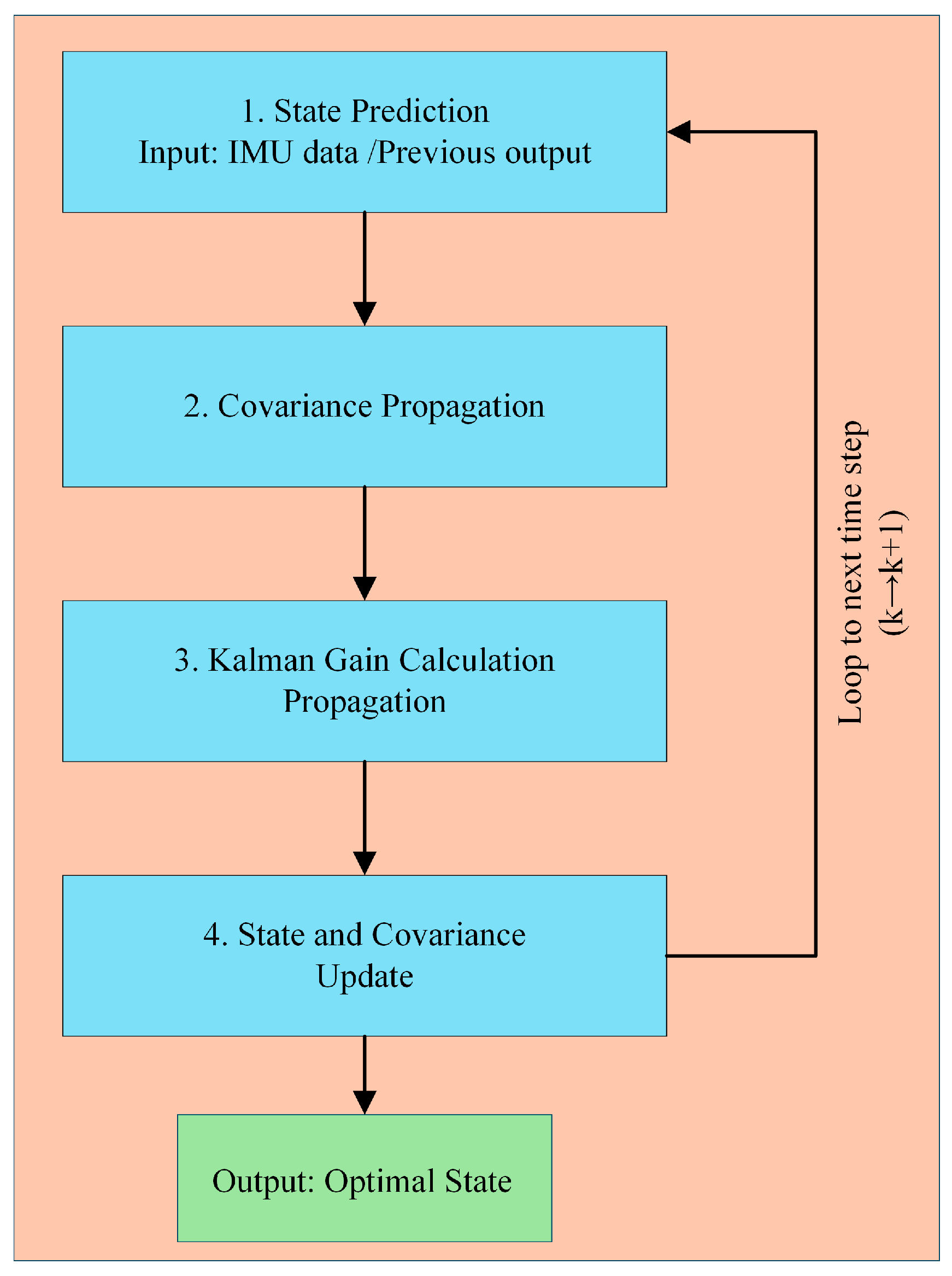
The EKF workflow, as shown in Figure 3, encompasses four key sequential steps: state prediction, covariance propagation, Kalman gain calculation, and state update. The state transition matrix $F$ incorporates coupling terms between attitude and velocity errors, originating from acceleration decomposition biases caused by misalignment angles. The observation matrix $H$ features a sparse structure, as only position $\delta p$ and velocity $\delta v^n$ errors are directly observable via GNSS, whereas attitude, bias, and synchronization errors are estimated indirectly. The “Loop to next time step” ensures the posterior state from the update step feeds back as input for the next iteration, enabling continuous navigation state estimation.

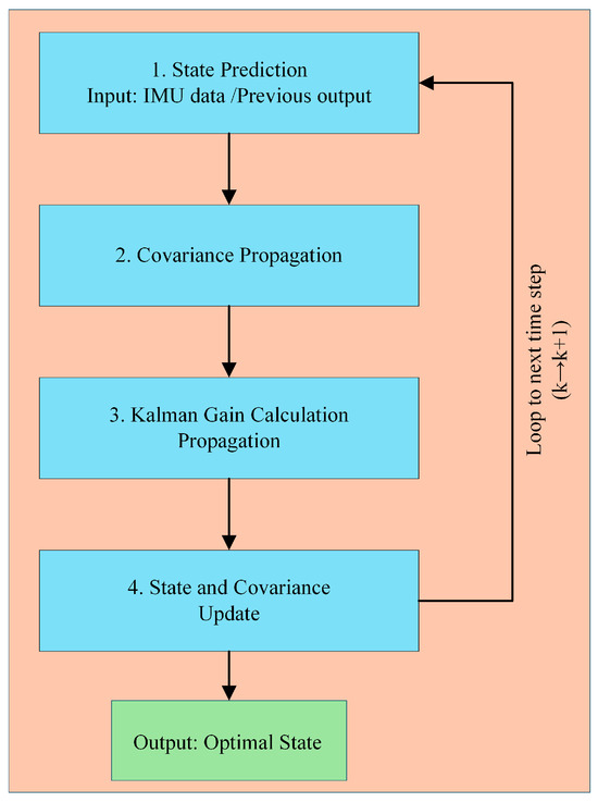
Figure 3. Workflow of the EKF for GNSS/INS integrated navigation.

Specifically, the EKF operates on an error-state vector explicitly designed to capture all critical deviations impacting navigation performance. This vector is defined as follows:

$$X={\left[\begin{array}{ccccccc}{\varphi }^T\hfill & {(\delta v^n)}^T\hfill & {(\delta p)}^T\hfill & {({\epsilon }^b)}^T\hfill & {({\nabla }^b)}^T\hfill & {(\delta l^b)}^T\hfill & \delta t\hfill \end{array}\right]}^T$$

(41)

where $\varphi$ denotes the attitude error, $\delta v^n$ represents the velocity error in the navigation frame, $\delta p$ is the position error, ${\epsilon }^b$ and ${\nabla }^b$ are the gyroscope and accelerometer biases in the body frame, respectively. $\delta l^b$ is the lever-arm error, and $\delta t$ characterizes the time synchronization error.

To contextualize this within the EKF workflow, the observation model quantifies discrepancies between INS and GNSS outputs, forming the measurement vector:

$$Z=\left[\begin{array}{c}{\tilde{v}}_{INS}^n-{\tilde{v}}_{GNSS}^n\\ {\tilde{p}}_{INS}-{\tilde{p}}_{GNSS}\end{array}\right]$$

(42)

where ${\tilde{v}}_{INS}^n$ and ${\tilde{v}}_{GNSS}^n$ are the north/east/up velocity estimates from the INS and GNSS, respectively.

This sparse structure directly reflects the physical relationship between error states and observations: only the velocity error $\delta v^n$ and position error $\delta p$ contribute to INS-GNSS residuals, with identity submatrices ${\mathrm{I}}_{3\times 3}$ ensuring direct mapping, while zeros indicate no direct contribution from attitude, bias, or synchronization errors.

The lever-arm error model and time desynchronization error model constructed above are used as state vectors to form the state space equation for integrated navigation, which is given by the following:

$$\left\{\begin{array}{l}\dot{X}=FX+G{W}^b\hfill \\ Z=HX+V\hfill \end{array}\right.$$

(43)

$$F=\left[\begin{array}{llllll}{M}_{aa}\hfill & M_{av}\hfill & M_{ap}\hfill & -C_b^n\hfill & 0_{3*3}\hfill & 0_{3*4}\hfill \\ M_{va}\hfill & M_{vv}\hfill & M_{vp}\hfill & 0_{3*3}\hfill & C_b^n\hfill & 0_{3*4}\hfill \\ 0_{3*3}\hfill & M_{pv}\hfill & M_{pp}\hfill & 0_{3*3}\hfill & 0_{3*3}\hfill & 0_{3*4}\hfill \\ 0_{10*3}\hfill & 0_{10*3}\hfill & 0_{10*3}\hfill & 0_{10*3}\hfill & 0_{10*3}\hfill & 0_{10*4}\hfill \end{array}\right]$$

(44)

$$G=\left[\begin{array}{ll}-C_b^n\hfill & 0_{3*3}\hfill \\ 0_{3*3}\hfill & C_b^n\hfill \\ 0_{13*3}\hfill & 0_{13*3}\hfill \end{array}\right]W^b=\left[\begin{array}{c}{w}_g^b\\ w_a^b\end{array}\right]$$

(45)

$$H=\left[\begin{array}{cccccc}{0}_{3*3}\hfill & I_{3*3}\hfill & 0_{3*3}\hfill & 0_{3*6}\hfill & -C_b^n({\omega }_{eb}^b\times )\hfill & a^n\hfill \\ 0_{3*3}\hfill & 0_{3*3}\hfill & I_{3*3}\hfill & 0_{3*6}\hfill & -M_{pv}{C}_b^n\hfill & M_{pv}{v}_{INS}^n\hfill \end{array}\right]V=\left[\begin{array}{c}{V}_v\\ V_p\end{array}\right]$$

(46)

where $F$ is the system transition matrix, $G$ is the process noise matrix, $W$ is the process noise (gyroscope white noise $w_g^b$ in rad/s and accelerometer white noise $w_a^b$ in m/s²), $H$ is the observation matrix, and $V$ is the observation noise (GNSS velocity white noise $V_v$ in m/s and GNSS position white noise $V_p$ in m).

The error model parameters are derived from hardware specifications: gyroscope bias (0.05 rad/s) and accelerometer bias (215 $\mathsf{\mu }\mathrm{g}$) correspond to the ATK1218-BD receiver and MPU6050 IMU used. The initial covariance matrix $P_0$ has diagonal elements: attitude error variance ${(1.2°)}^2$, velocity error variance ${(0.01\mathrm{m}/\mathrm{s})}^2$, and matching misalignment errors from initial alignment. The simulation frequency of 100 Hz aligns with the actual sampling rate of onboard sensors, ensuring consistency between simulation and real-world execution.

The state transition and observation processes are governed by the following discrete-time equations:

$$\left\{\begin{array}{l}{X}_{k|k-1}=F_{k-1}{X}_{k-1|k-1}+G_{k-1}{W}_{k-1}\hfill \\ Z_k=H_k{X}_{k|k-1}+V_k\hfill \end{array}\right.$$

(47)

where $F_{k-1}$ is the system transition matrix at time $k-1$, $G_{k-1}$ is the system noise matrix at time $k-1$; $W_{k-1}$ is the system excitation noise sequence at time $k-1$.

In implementing the EKF, the process noise covariance matrix $Q$ and the measurement noise covariance matrix $R$ were initially set based on sensor specifications and further refined through an empirical tuning process. The initial values of $Q$ were determined by considering the sensor characteristics, where the gyroscope bias was set to 0.05$°/\mathrm{s}$ and the accelerometer bias was set to 215 $\mathsf{\mu }\mathrm{g}$ $(0.215{\mathrm{m}/\mathrm{s}}^2)$, consistent with the performance specifications of the MEMS inertial sensors utilized in the system. This initial setup of $Q$ aims to enhance system stability and mitigate excessive state—estimation fluctuations. Meanwhile, $R$ is initially configured to reflect nominal GNSS measurement uncertainty.

However, to cope with real-world dynamics, $Q$ is dynamically adjusted to account for sensor drift and unpredictable noise growth, which is critical for maintaining filter consistency and preventing divergence under changing operational conditions. The filter monitors the rate of change of estimated biases (${\epsilon }^b$ for gyroscopes, ${\nabla }^b$ for accelerometers). If the magnitude of the bias estimate exceeds a predefined threshold (gyroscope bias threshold: 0.01 rad/s; accelerometer bias threshold: 10 mg, set based on manufacturer specifications and empirical testing for MEMS—grade sensors) for a sustained period, it indicates potential sensor drift. When drift is detected, $Q$ is scaled using a multiplicative factor $\gamma$ derived from the innovation sequence and residual analysis:

$$\gamma =1+\alpha ({\displaystyle \frac{‖{\epsilon }^b‖}{‖{\sigma }_{\epsilon }‖}}+{\displaystyle \frac{‖{\nabla }^b‖}{‖{\sigma }_{\nabla }‖}})$$

(48)

where $\alpha =0.2$, ${\sigma }_{\epsilon }=0.05\mathrm{rad}/\mathrm{s}$, and ${\sigma }_{\nabla }=215\mathrm{mg}$. The updated covariance becomes

$$Q_{\mathrm{updated}}=\gamma \cdot Q_{\mathrm{nominal}}$$

(49)

This expansion of $Q$ explicitly accounts for amplified stochastic errors during drift, enhancing the filter’s ability to track sudden error dynamics and ensuring robustness under transient sensor instability.

The measurement-noise covariance matrix $R$ is initialized to reflect nominal GNSS uncertainty and adapted to varying signal conditions using two complementary indicators: dilution of precision (DOP) and innovation consistency checks. Position dilution of precision (PDOP) exceeding 6 signals poor satellite geometry, triggering proportional scaling relative to a nominal PDOP of 2.5 (typical for open-sky conditions). Concurrently, the Mahalanobis distance is as follows:

$$d_k=\sqrt{{(Z_k-H_k{\widehat{X}}_{k|k-1})}^T{S}_k^{-1}(Z_k-H_k{\widehat{X}}_{k|k-1})}$$

(50)

where $S_k=H_k{P}_{k|k-1}{H}_k^T+R_k$, is used to detect measurement inconsistency, with sustained $d_k>3$ indicating issues like multipath interference. The updated $R$ is given by the following:

$$R_{\mathrm{updated}}=\max (\beta \cdot {\displaystyle \frac{\mathrm{PDOP}}{{\mathrm{PDOP}}_{\mathrm{nominal}}}},\eta )\cdot R_{\mathrm{nominal}}$$

(51)

where $\beta =1.5$ and $\eta =2$ ensure a minimum scaling to avoid over-reliance on noisy measurements.

The EKF implements these adaptations through iterative prediction and update steps. In the prediction phase, the a priori state and covariance are propagated as follows:

$$\left\{\begin{array}{l}{\widehat{X}}_{k|k-1}=F_k{\widehat{X}}_{k-1}\hfill \\ P_{k|k-1}=F_k{P}_{k-1}{F_k}^T+G_k{Q}_k{G_k}^T\hfill \end{array}\right.$$

(52)

In the update phase, the Kalman gain is computed as follows:

$$K_k=P_{k|k-1}{H_k}^T{(H_k{P}_{k|k-1}{H_k}^T+R_k)}^{-1}$$

(53)

The state estimation is updated through the Kalman gain matrix:

$$\left\{\begin{array}{l}{\widehat{X}}_k={\widehat{X}}_{k|k-1}+K_k(Z_k-H_k{\widehat{X}}_{k|k-1})\hfill \\ {\widehat{P}}_k=(I-K_k{H}_k){\widehat{P}}_{k|k-1}\hfill \end{array}\right.$$

(54)

where $X_{k|k-1}$ is the state estimate at time $k-1$, $K_k$ is the Kalman gain matrix, $Z_k$ is the new observation data at time $k$, $H_k$ is the observation matrix, $P_{k|k-1}$ is the covariance matrix of the state estimate at time $k-1$, and $P_{k|k}$ is the covariance matrix of the updated state estimate at time $k$.

5. Simulation and Experiment Results

5.1. Simulation Results

5.1.1. Differential Positioning System Simulation

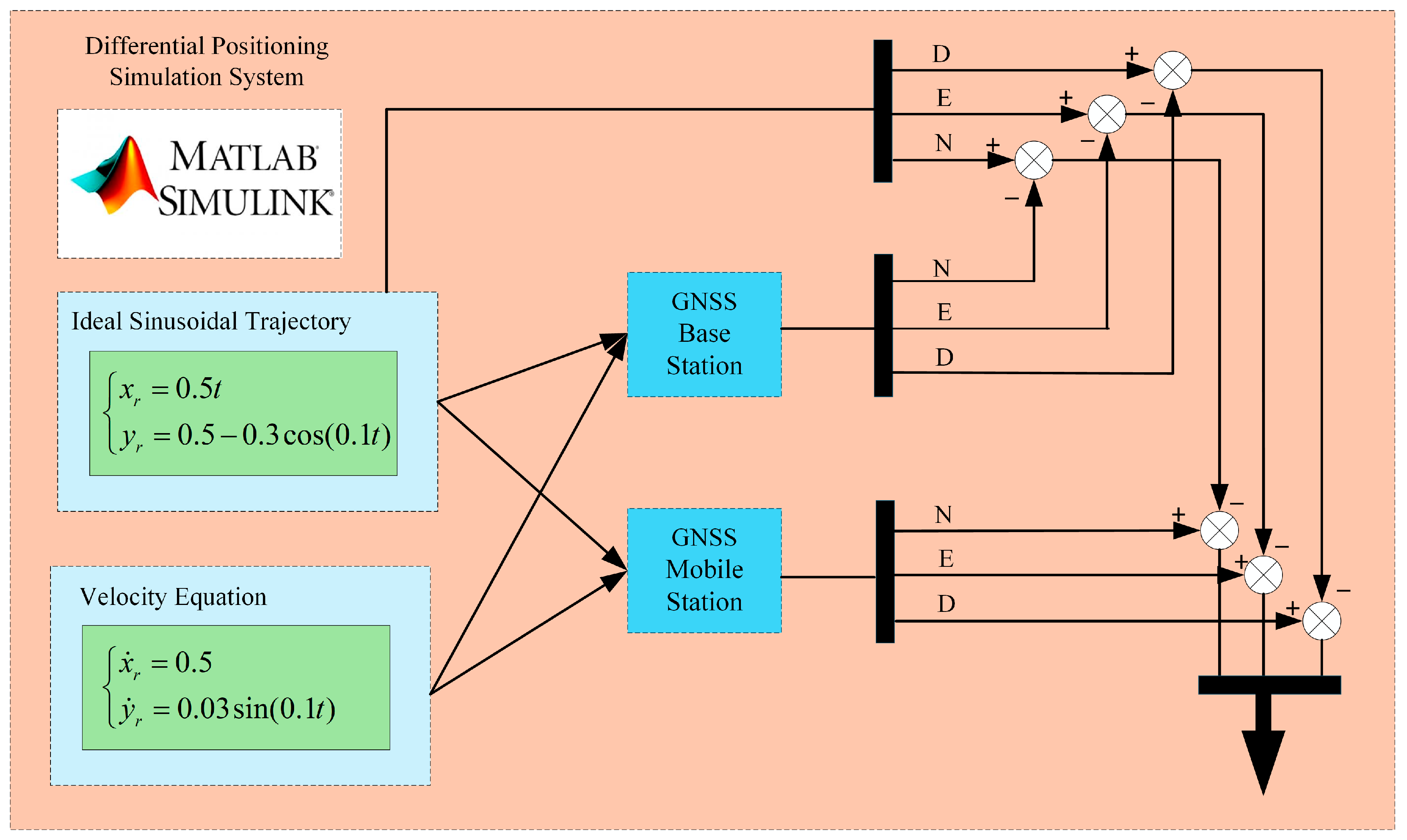
The GNSS receiver simulation system is designed to simulate real-world positioning challenges, including multipath interference, satellite signal variability, and sensor noise, to evaluate the proposed framework under common environmental influences on positioning accuracy. The simulation incorporates differential positioning corrections, which effectively mitigate systematic GNSS errors such as satellite clock bias and atmospheric delays. By evaluating positioning performance under controlled conditions that reflect typical sources of positioning errors, this system provides valuable insights into the effectiveness of the proposed GNSS/INS integration framework before real-world deployment.

By evaluating positioning performance under controlled conditions, this system provides valuable insights into the effectiveness of GNSS/INS integration before real-world deployment. The overall simulation framework is illustrated in Figure 3.

The receiver’s input parameters include position and velocity, which can be defined in either the Cartesian or geodetic coordinate system (latitude, longitude, and altitude). The output parameters include position, velocity, horizontal velocity (representing the two-dimensional motion on the ground), and heading (the horizontal direction of movement), all expressed in the geodetic coordinate system.

The position coordinate system is set to the Cartesian coordinate system, with horizontal accuracy errors of 0.1, vertical accuracy errors of 0.5, and velocity errors of 0.01. The attenuation factor is set to 0.5, the randomness parameter to 28, and the epoch time to 93 s. The simulation results are shown in Figure 4.

Figure 4. Differential positioning simulation system.

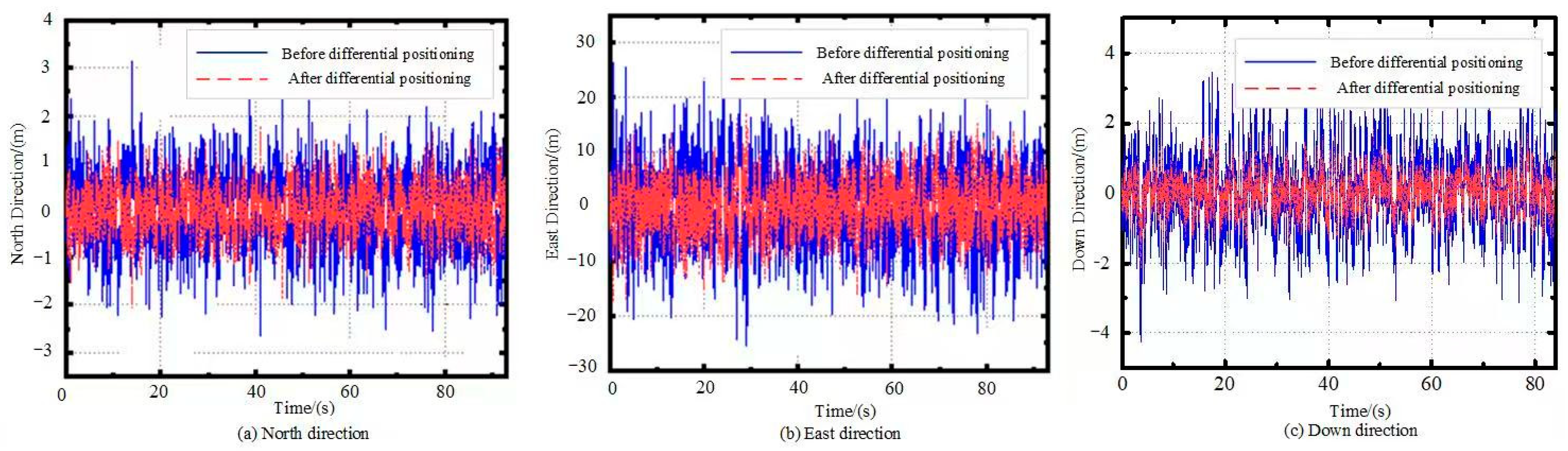
Figure 5 compares the positioning errors in three orthogonal directions. The blue lines represent the difference between the mobile station GNSS receiver and the ideal trajectory before applying differential positioning, while the red lines show the difference after applying differential positioning. An accuracy improvement of approximately 1 m is observed in the north direction.

Figure 5. Error comparison before and after differential positioning.

It can be observed that after differential positioning, the GNSS receiver at the mobile station exhibits certain improvements in the east and north directions while mitigating some systematic errors. It can be observed that after differential positioning, the GNSS receiver at the mobile station exhibits certain improvements in the east and north directions while mitigating some systematic errors.

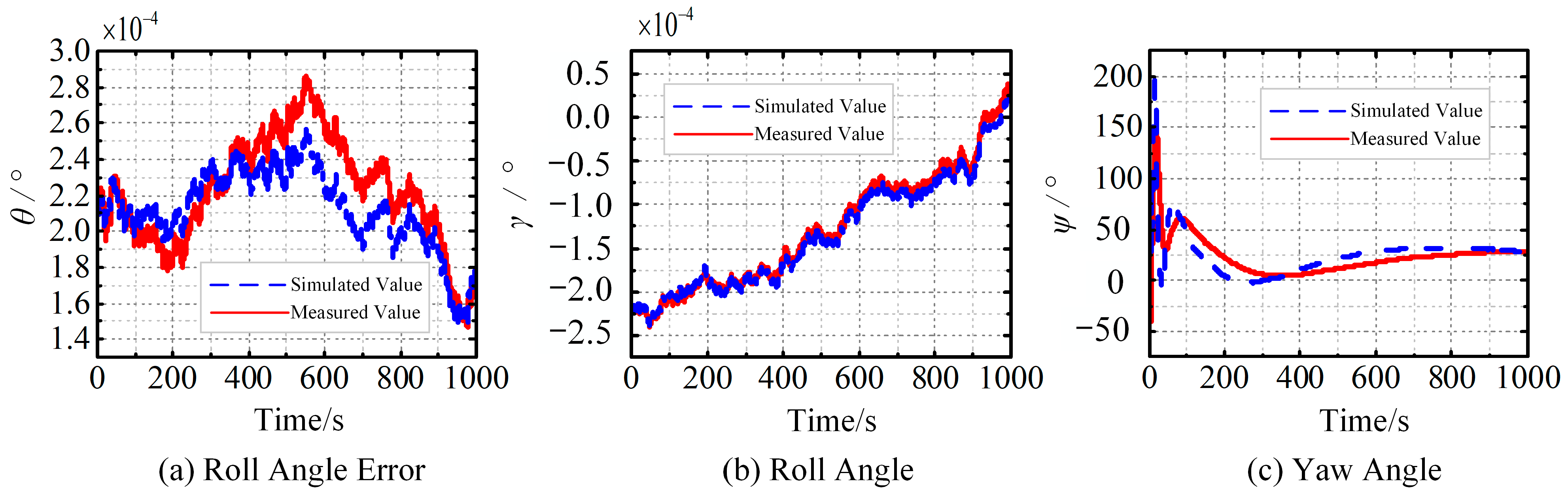
5.1.2. Simulation of Initial Alignment for Inertial Navigation

The initial alignment simulation of inertial navigation is conducted under static base conditions. The process is divided into a coarse alignment phase and a fine alignment phase.

For initialization, all attitude angles are set to 0, velocity parameters are set to (0, 0, 0), and position parameters are also set to (0, 0, 0). The initial misalignment angles are assigned as 1.2° for north and 5° for east, which are representative of realistic mounting errors encountered in vehicle-mounted INS systems. The gyro bias is set to 0.05 $\mathsf{\mu }\mathrm{g}$, and the accelerometer bias is set to 215 $\mathsf{\mu }\mathrm{g}$, values that align with the typical specifications of MEMS inertial sensors commonly used in navigation applications. The gyroscope random walk is set to 0.008$°/\mathrm{h}$, while the accelerometer random walk is set to 1.09 $\mathsf{\mu }\mathrm{g}$, simulating the stochastic noise characteristics observed in real-world IMU systems. The attitude errors are initialized as 0.8°, 0.7°, and 50°, and the velocity error is 0.01 $\mathrm{m}/\mathrm{s}$ in all three axes. The total simulation time is 1000 s, with an update interval of 0.1 s. These settings ensure that the simulation captures practical error characteristics that impact GNSS/INS integration performance, providing a reliable basis for evaluating the proposed approach.

The fine alignment results are as follows (Figure 6):

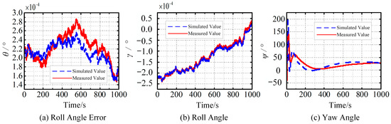
Figure 6. Simulation results of initial alignment.

The nominal attitude angles are initially set to 0. After the coarse alignment phase, the roll, pitch, and yaw angles converge to $2.1235\times {10}^{-4}°$, $-2.1864\times {10}^{-4}°$, and $0.00659°$, respectively. Following 1000 s of fine alignment, these angles further refine to $1.74905\times {10}^{-4}°$, $1.61903\times {10}^{-5}°$, and $0.0028°$, respectively. After the Kalman filtering correction, the misalignment errors are effectively reduced to an acceptable range, providing a more accurate initial attitude for subsequent navigation.

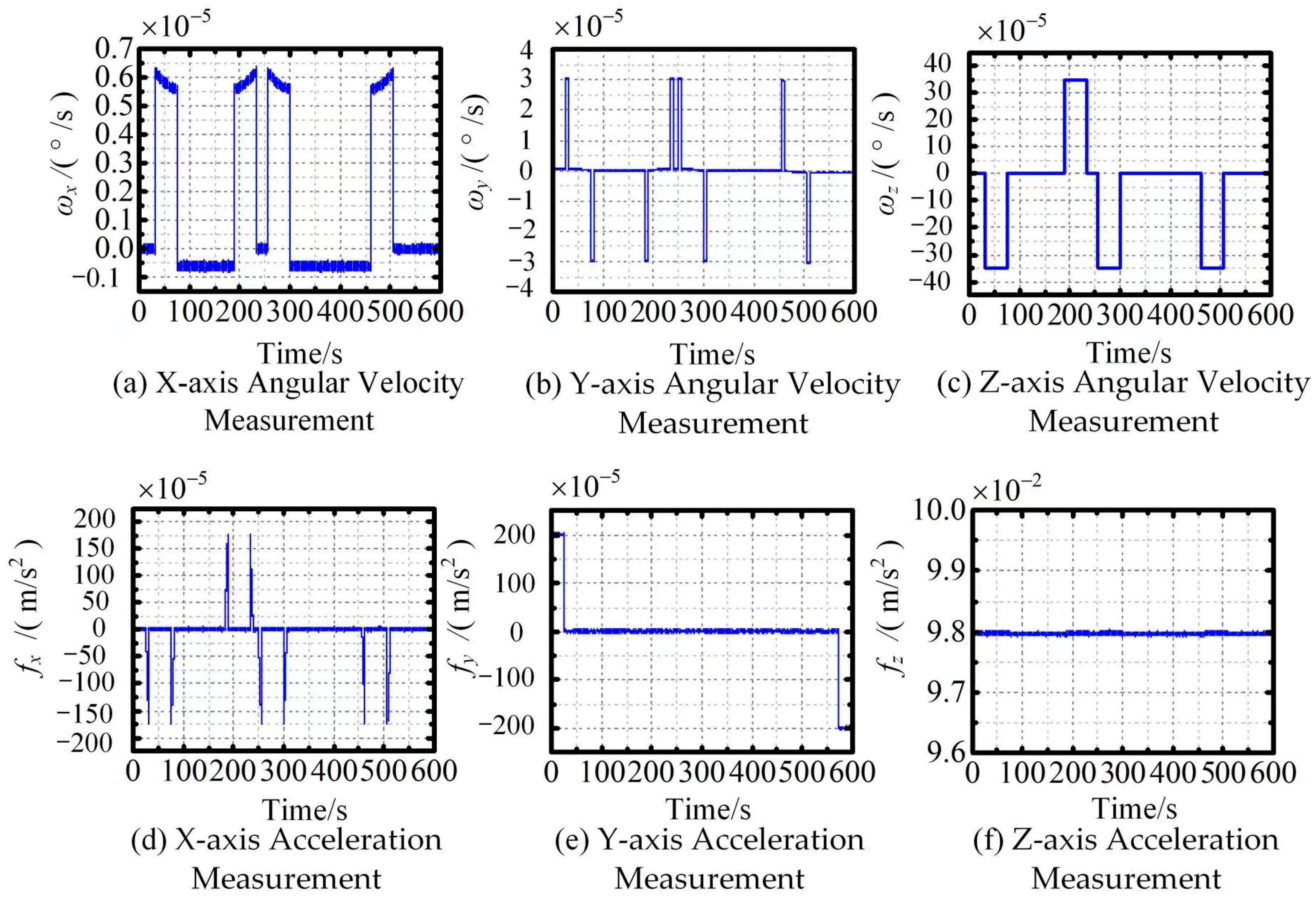
5.1.3. Inertial Navigation Simulation

The update frequency is set to $100\mathrm{Hz}$, the measurement range of the accelerometer is $\pm 8 \mathrm{g}$, the constant bias noise of the accelerometer is 28 $\mathsf{\mu }\mathrm{g}$. the random noise of the accelerometer is $8 \mathsf{\mu }\mathrm{g}/\sqrt{\mathrm{Hz}}$, the measurement range of the gyroscope is $\pm 180°/\mathrm{s}$, the constant bias noise of the gyroscope is 0.01 $°/\mathrm{h}$, and the random noise of the gyroscope is 0.0018 $(°/\mathrm{h})/\sqrt{\mathrm{Hz}}$. The lever-arm error is set to 1 m, and the time desynchronization error is set to 0.2 s. The vehicle is set to accelerate at a speed of 0.2 ${\mathrm{m}/\mathrm{s}}^2$ for 25 s, travel in a straight line, and turn right at an angular velocity of 2° per second for 45 s, maintain a straight-line travel at a speed of 5 m/s for 100 s, then turn left at an angular velocity of 2° per second for 45 s, maintain a straight-line travel at a speed of 5 m/s for 10 s, turn right at an angular velocity of 2° per second for 45 s, maintain straight-line travel for 150 s, then turn right at an angular velocity of 2° per second for 45 s, maintain straight-line travel for 60 s, and finally decelerate at a speed of 0.2 ${\mathrm{m}/\mathrm{s}}^2$ for 25 s, returning to the initial point with a speed of 0.

The measurement results of the IMU during the simulation are as follows (Figure 7):

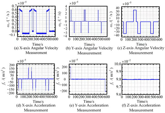
Figure 7. IMU measurement results.

It is evident that the pure IMU exhibits high precision during the simulation measurement phase, with its accuracy in attitude reaching the level of ${10}^{-5}°/\mathrm{s}$, and its horizontal acceleration accuracy reaching the level of ${10}^{-5}{\mathrm{m}/\mathrm{s}}^2$. The measurement results of GNSS during the simulation are as follows (Figure 8):

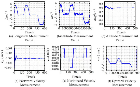
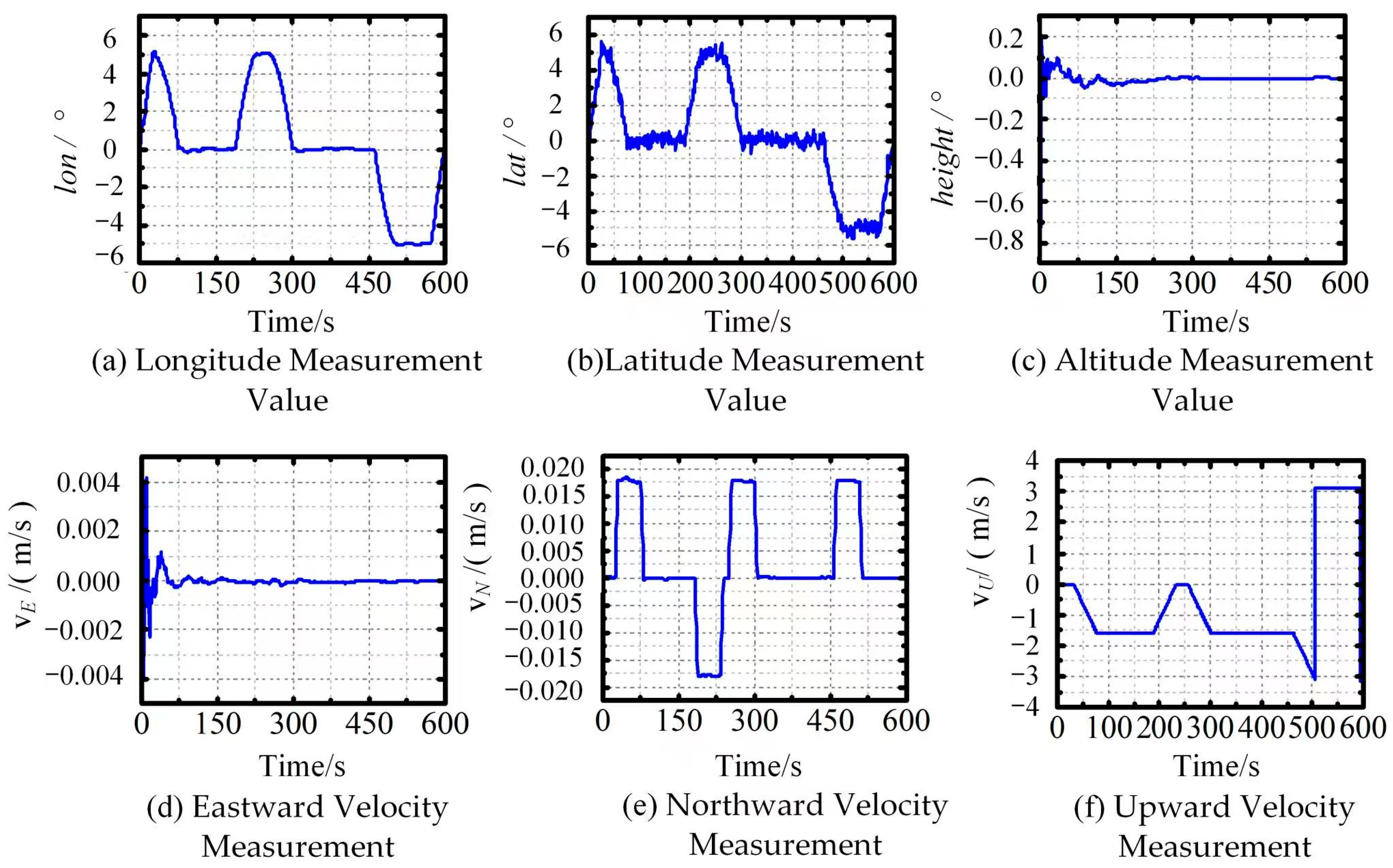
Figure 8. GNNS measurement results.

By comparing the figures, it is evident that the measurement accuracy of GNSS is lower compared to that of the IMU. The velocity accuracy of GNSS is at the level of 0.001 m/s, and its position accuracy is at the level of 5 m.

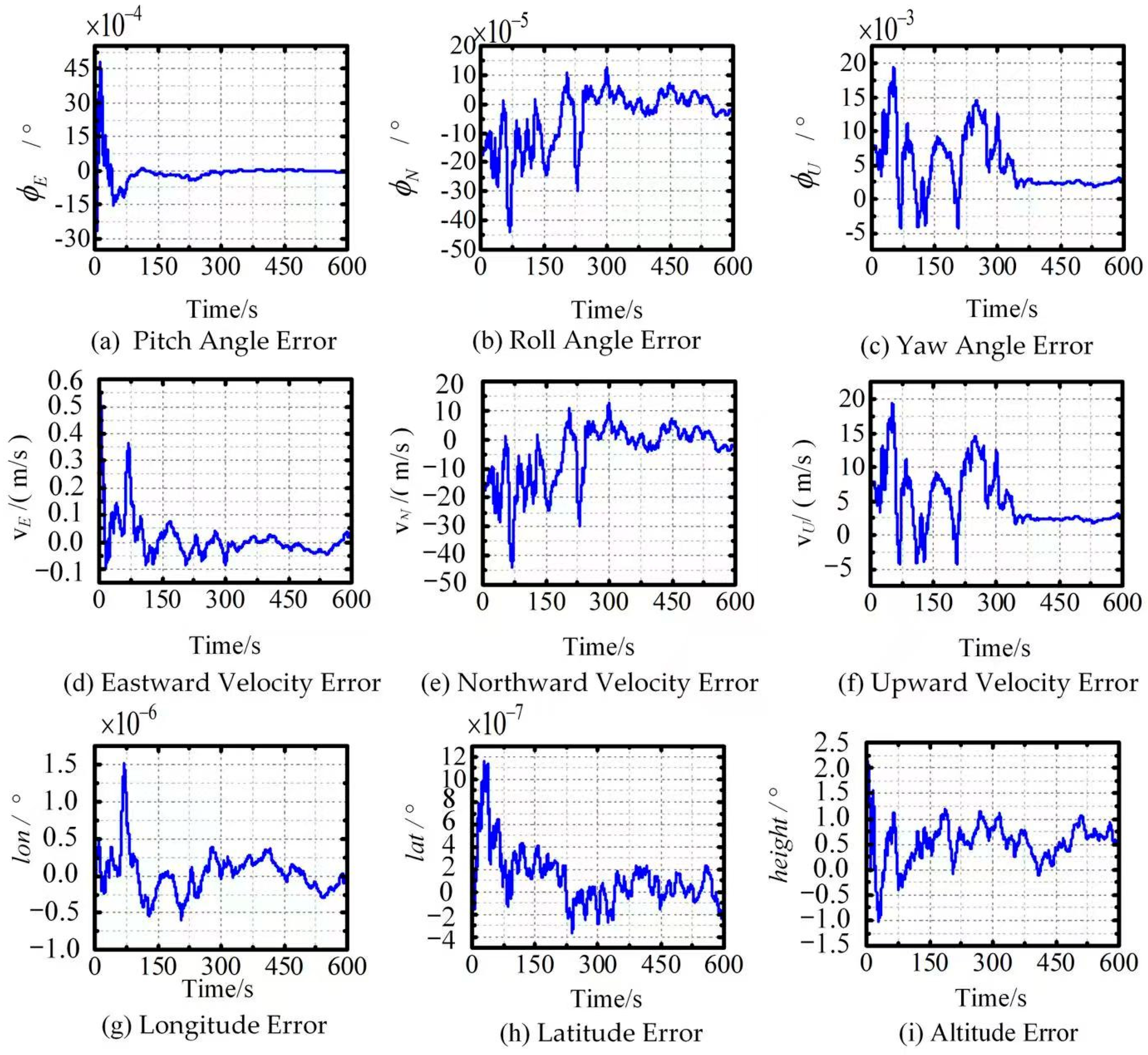
During the integrated navigation process, the results of various types of errors are as follows:

Figure 9 illustrates the navigation errors in the integrated INS/GNSS system. It is evident that through integrated navigation, the stability of the vehicle positioning system can be effectively enhanced, mitigating the cumulative errors of the IMU and improving the positioning accuracy of GNSS. In terms of misalignment angle errors, fluctuations occur at levels of 5 × 10⁻⁶, 2 × 10⁻⁵, and 0.06° for pitch, roll, and yaw angles, respectively, and converge rapidly. At the velocity error level, there is an initial fluctuation of 0.5 in the eastward direction, which quickly converges to within ±0.15 m/s; in the northward direction, there is an initial fluctuation of 10 m/s, which also converges to within ±0.15 m/s. Therefore, considering the lever-arm errors and time desynchronization errors, the EKF can be effectively utilized to achieve improved positioning capabilities in the integrated navigation system.

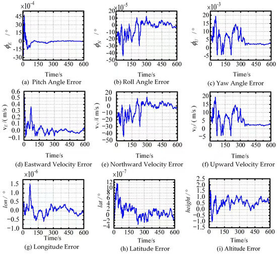
Figure 9. Navigation errors.

5.1.4. Integrated Navigation Trajectory

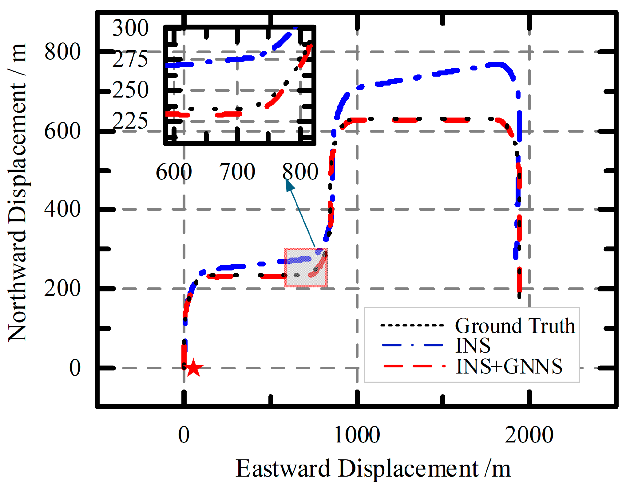
The integrated navigation trajectory is shown in Figure 10 below:

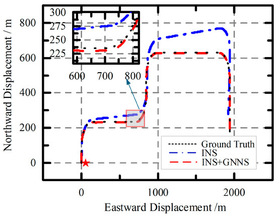
Figure 10. Comparison chart of integrated navigation trajectory.

In Figure 10, the black dashed line represents the ground truth of the integrated navigation trajectory, the blue dash-dot line represents the trajectory of pure IMU-based navigation, and the red dashed line represents the trajectory after GNSS/INS integration. It can be observed that under pure IMU-based navigation, the navigation solution quickly diverges. With integrated navigation, the vehicle can effectively track the desired path, maintaining navigation accuracy within 2 m, demonstrating high tracking accuracy.

The results indicate that the adaptive tuning of the process noise covariance matrix Q and measurement noise covariance matrix R in the EKF enhances the stability of state estimation. Compared to the baseline INS configuration, the optimized EKF exhibits superior performance in alleviating horizontal positioning errors and curbing the cumulative drift of the IMU. This confirms that the integration of GNSS and INS with an adaptively tuned EKF bolsters navigation robustness, providing reliable state estimation in practical navigation scenarios.

Although we were unable to include a direct comparison with established benchmark datasets such as KITTI due to the specific nature of our experimental setup, our simulation and experimental results provide strong evidence of the proposed method’s effectiveness. The proposed method integrates real-time differential GNSS corrections and an adaptive EKF to dynamically reduce positioning errors and mitigate INS error accumulation. This combination of techniques significantly enhances the robustness and precision of the navigation system in practical navigation scenarios.

5.2. Instrumentation and Experimental Platform Setup

5.2.1. GNSS Positioning Module

SPP is one of the most easily implemented and fastest satellite positioning methods. However, its accuracy varies significantly due to differences in positioning chips, antenna reception methods, antenna types, and data processing algorithms. In addition to being affected by systematic biases, SPP is also influenced by the receiver’s hardware conditions, leading to substantial variations in positioning accuracy under different scenarios. Despite these limitations, SPP devices can be effectively utilized to establish a differential positioning system, mitigating certain systematic errors. After applying differential positioning, the accuracy of the mobile station GPS receiver is significantly improved. This study analyzes positioning results with and without differential positioning through experimental validation to demonstrate its effectiveness.

To minimize receiver-related errors, we use identical positioning modules in the experiment, ensuring consistency in data output frequency. The selected module is the dual-mode GNSS positioning module ATK1218-BD, which supports GNSS+BDS single-frequency positioning. Since single-frequency positioning inherently compensates for ionospheric errors, its positioning accuracy can be maintained within a range of 4–10 m. Additionally, this module is compact, cost-effective, and comes with dedicated software for data logging, making it highly suitable for low-cost vehicle-mounted positioning systems.

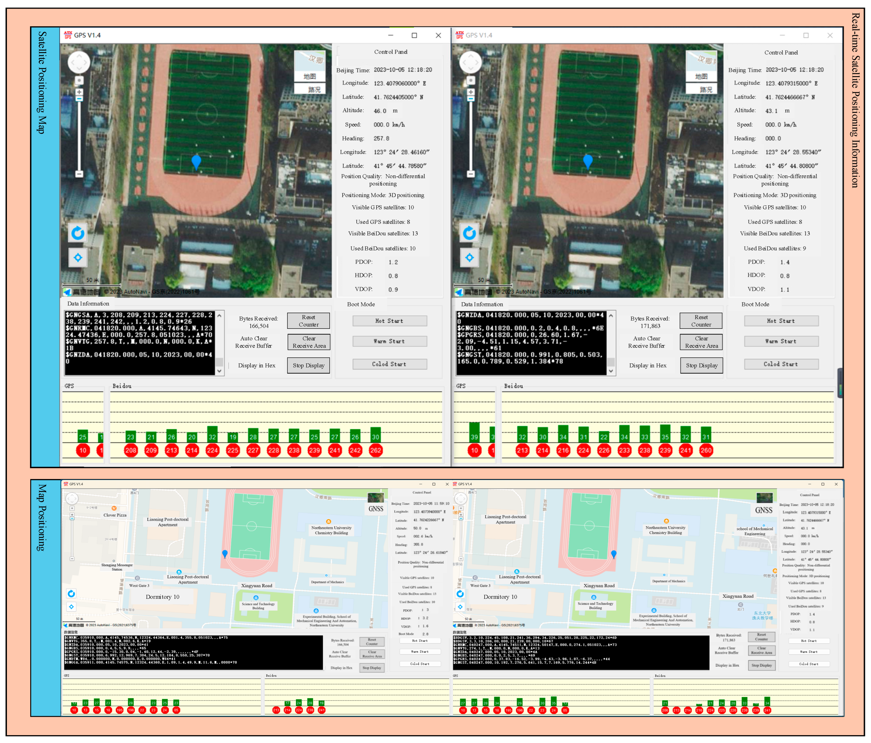
In the GNSS positioning experiment, the NMEA-0183 protocol provides additional information beyond UTC and latitude/longitude, including the number of visible satellites and the dilution of precision (DOP) factor. By incorporating this supplementary data, the accuracy of single-point positioning can be improved, thereby enhancing the overall positioning performance. The GPS information panel parsed from the NMEA-0183 protocol is shown in Figure 11:

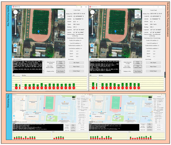
Figure 11. GNNS single point positioning information.

5.2.2. Experimental Platform Setup

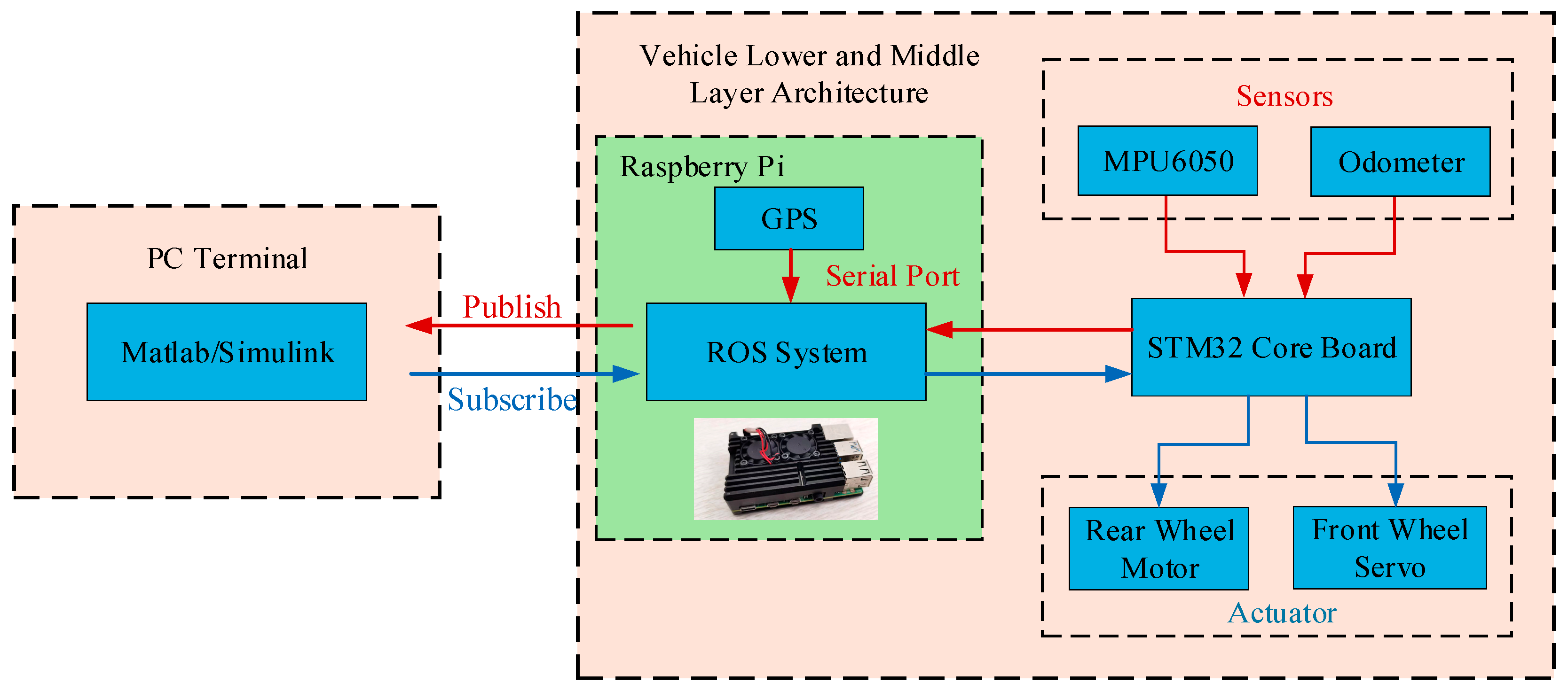
The experimental platform is divided into three layers: the lower, middle, and upper layers. The lower layer consists of a specific brand of Ackermann mobile vehicle chassis, serving as the controlled object. The middle level employs a Raspberry Pi running the Robot Operating System (ROS) to manage communication and control between the upper and lower levels. The upper level is responsible for implementing the controller in MATLAB/Simulink R2021b, which provides ideal trajectory information and control commands.

In the experiment, the ATK1218-BD module supplies GNSS positioning data, while the MPU6050 module, mounted on the vehicle chassis, provides speed and attitude information. These two data sources are integrated for navigation. Specifically, the GNSS module delivers latitude, longitude, and time information, whereas the IMU module provides attitude and velocity data. Both sets of information are transmitted to the ROS module on the middle layer, where data fusion for integrated navigation is performed. This fusion process directly implements the adaptive EKF algorithm from Section 4.2, enabling real-time compensation for sensor errors and temporal discrepancies. The upper-level PC subscribes to ROS topics to retrieve the fused navigation data for further analysis. The experimental vehicle system is shown in Figure 12.

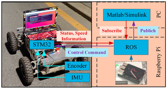
Figure 12. The experimental vehicle system.

The lower layer executes control commands from the upper layers to ensure stable vehicle movement. It includes dual-wheel motors, encoders, and an MPU6050 IMU for motion control and navigation. Speed is regulated using encoder feedback processed through a PID algorithm, with PWM signals adjusting motor output. The IMU provides real-time orientation data, enabling closed-loop control for precise trajectory tracking. The ROS module in the middle layer fuses GNSS and IMU data for improved localization, publishing navigation information for the upper-layer MATLAB/Simulink controller to process in real time. This hierarchical structure ensures efficient motion control and navigation integration.

The middle layer is implemented on a Raspberry Pi running the ROS system, primarily handling communication between the lower and upper layers. It receives control commands from the upper layer, transmits them to the lower layer, and processes navigation data. Communication between the middle and upper layers is established using IP and SSH protocols, facilitating smooth interaction between ROS and MATLAB for data exchange during experiments. ROS operates on a publisher–subscriber mechanism, ensuring efficient data transmission. The middle layer receives commands from the upper layer, such as velocity and steering angle, and relays them to the lower layer for execution. Simultaneously, it fuses sensor data (including GNSS position, IMU attitude, and velocity information) and forwards the integrated results to the upper layer for trajectory tracking and control optimization. By streamlining command transmission and data fusion, the middle layer ensures real-time responsiveness and facilitates precise vehicle navigation. This real-time data processing capability is essential for evaluating the system’s performance in practical navigation scenarios, where consistent and accurate data handling supports reliable positioning and control.

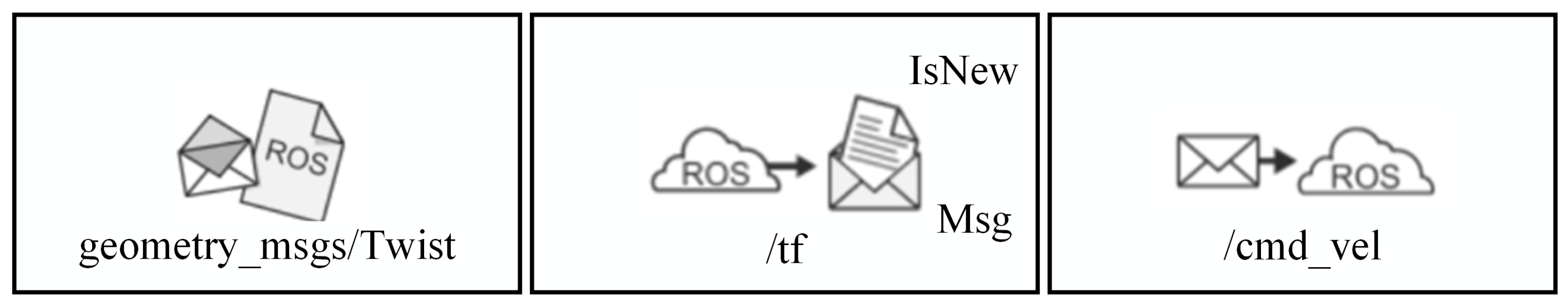
The upper layer is primarily based on the MATLAB/Simulink system running on a PC. It processes sensor feedback from the lower and middle layers while providing simulation filtering and control strategies. The built-in ROS toolbox in Simulink facilitates data communication, enabling message subscription and publication within the ROS network. The module structure is shown in Figure 13.

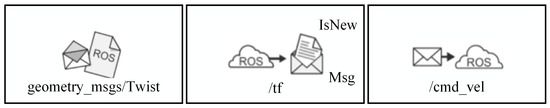
Figure 13. Simulink and ROS interaction module.

Through this module, the upper layer establishes a connection with the Raspberry Pi running ROS and communicates with the STM32 hardware to transmit precise control commands. The overall control architecture is illustrated in Figure 14.

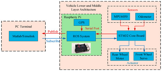
Figure 14. Vehicle bottom motion relationship.

This design ensures seamless integration between the simulation environment and real-world execution, improving system robustness and control accuracy.

5.3. Experimental Verification

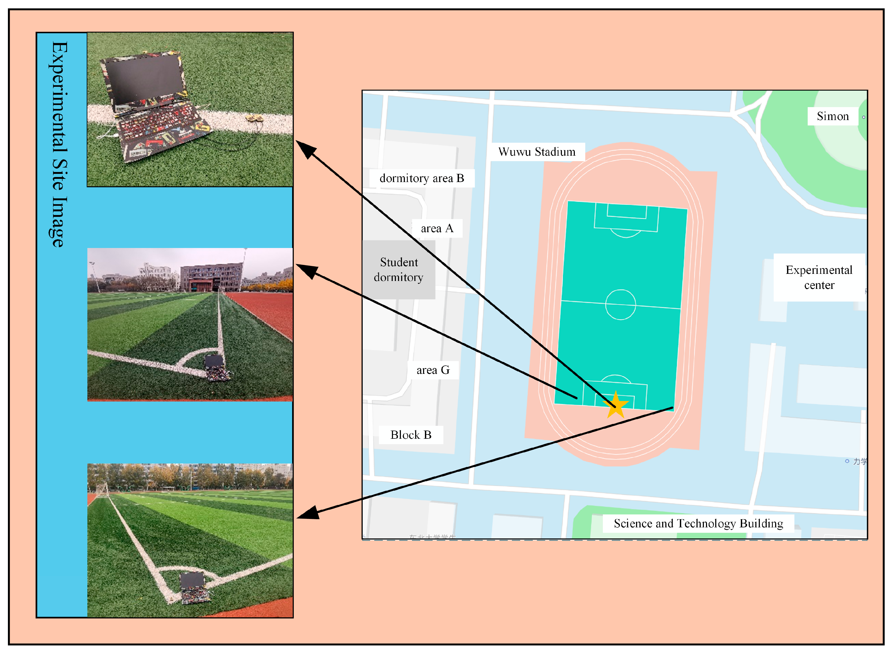
The experiment was conducted at the sports field on the west side of Northeastern University, with the midpoint of the southern goalpost serving as the positioning reference. This site was selected to balance controlled experimental conditions with the inclusion of typical environmental factors that may affect GNSS positioning: partial signal occlusion from surrounding trees and temporary structures, along with occasional crowd movement in the vicinity. These elements provided a practical testing scenario to evaluate the proposed framework’s performance under common real-world conditions. The setup allowed for a reliable assessment of the integration method’s ability to maintain positioning accuracy in the presence of mild environmental interference, ensuring the results reflect its performance in everyday navigation contexts.

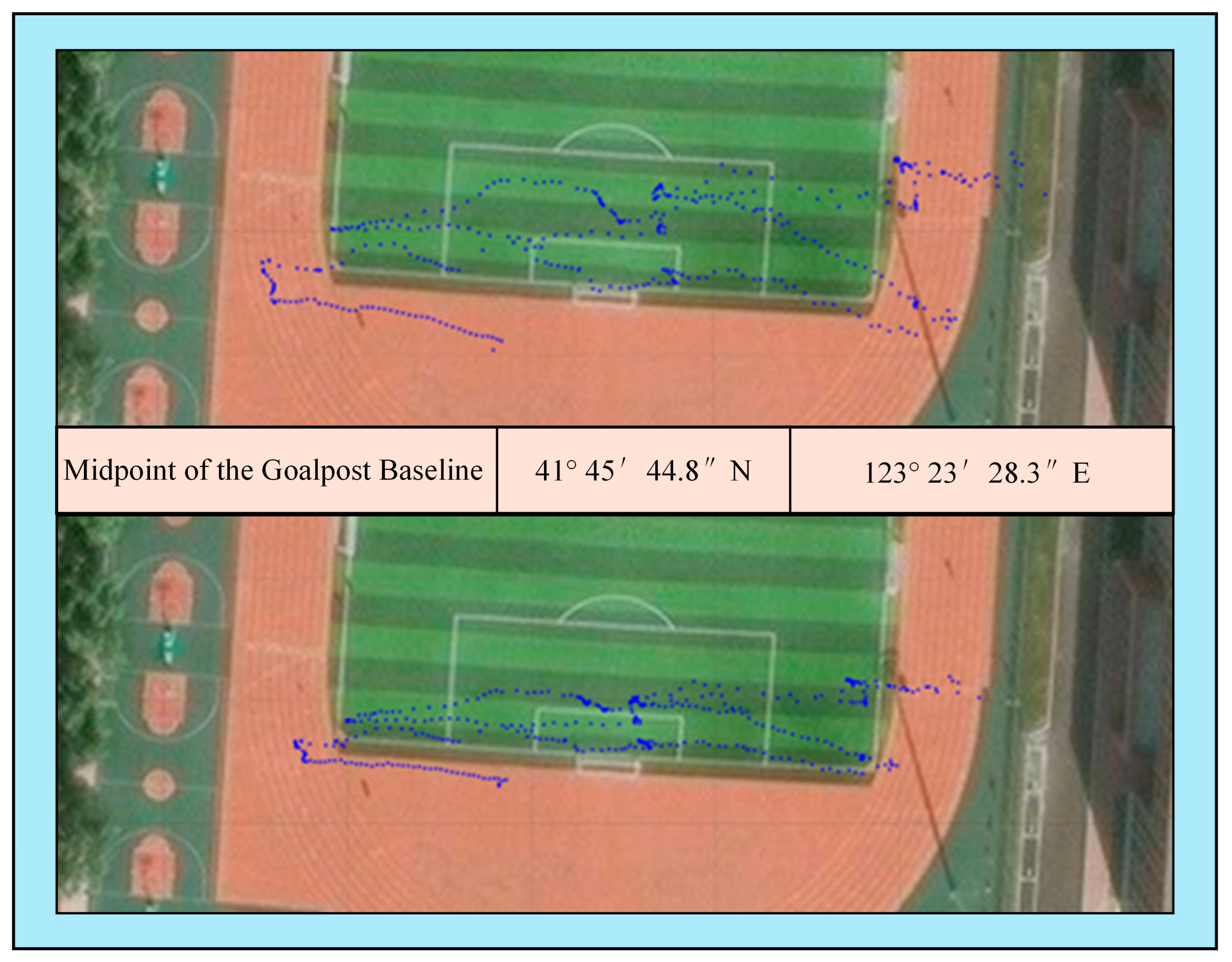
The latitude and longitude of this point were obtained from an online map: 123°23′28.3″ E, 41°45′44.8″ N. To verify the effectiveness of the differential positioning algorithm, the experiment started from the midpoint of the goalpost, proceeded to the west point on the goalpost baseline, paused, returned to the midpoint of the goalpost, paused again, then proceeded to the east point on the goalpost baseline, and repeated this route three times. The experimental positioning environment is shown in Figure 15:

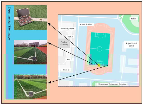
Figure 15. Experimental environment.

After conducting the baseline movement experiment through the goalpost, the positioning results are shown in Figure 16 below:

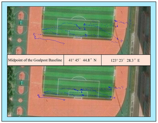
Figure 16. Comparison of differential experiments in experimental environments.

As shown in Figure 16, after differential positioning, the positioning information of the points where the vehicle stayed, including the west side of the goalpost baseline, the midpoint of the goalpost baseline, and the east side of the goalpost baseline, has significantly improved compared to before differential positioning.

Upon calculation, the maximum positioning accuracy improvement is approximately 4.2 m, thereby verifying the effectiveness of the differential positioning algorithm.

The experimental validation of the proposed GNSS/INS integrated navigation system was conducted in a controlled environment designed to simulate real-world challenges of weak GNSS signals. The experimental validation of the proposed GNSS/INS integrated navigation system was conducted in a controlled environment simulating real-world challenges of weak GNSS signals. The proposed framework, combining real-time differential GNSS corrections with an adaptive EKF, demonstrated robust performance under these conditions.

Key advancements were achieved through differential positioning technology and adaptive Kalman filter optimization. By employing a low-cost dual-frequency GNSS module (ATK1218-BD), the system reduced systematic errors such as ionospheric delays, achieving a positioning accuracy improvement of 4.2 m. This performance matches high-end differential systems while significantly lowering hardware costs. Dynamic error correction strategies further enhanced convergence speed, as evidenced by rapid error damping in north and east directions during simulated frequent-turn maneuvers. For integrated navigation, adaptive tuning of the Kalman filter’s process noise covariance matrix ($Q$) and measurement noise covariance matrix ($R$) enabled stable state estimation under dynamic conditions. The eastward velocity error converged to 0.5 m/s, and horizontal positioning accuracy remained within 2 m—results comparable to tightly coupled systems but achieved without the computational burden of pseudo-range or carrier-phase fusion.

However, some limitations remain. Multipath suppression in dense urban environments requires further refinement, and integrity risks such as signal spoofing were not fully addressed. Future work will prioritize testing in challenging scenarios like urban canyons and tunnels.

6. Conclusions

This study proposes an enhanced GNSS/INS integration framework that combines real-time differential GNSS corrections with an adaptive EKF, aiming to improve positioning accuracy in practical navigation scenarios. The framework leverages differential corrections to reduce positioning errors and employs the EKF to dynamically compensate for inertial sensor drift, misalignment angles, and time synchronization discrepancies.

The effectiveness of our proposed GNSS/INS integration framework was thoroughly validated through both simulation and controlled field experiments. As demonstrated in Figure 9, the framework significantly mitigated velocity errors, reducing initial fluctuations of 0.5 m/s in the eastward direction and 10 m/s in the northward direction to within ±0.15 m/s after convergence. Misalignment angle errors were effectively minimized, with pitch, roll, and yaw angles converging rapidly to levels of 5 × 10⁻⁶, 2 × 10⁻⁵, and 0.06°, respectively. Figure 10 further illustrates the system’s high tracking accuracy, maintaining navigation within 2 m of the desired path, achieving a maximum accuracy improvement of 4.2 m compared to conventional single-point positioning. These results underscore the practical efficacy of the proposed approach in real-world navigation scenarios.

The integration of an inertial sensor error model, which accounts for gyroscope bias, accelerometer bias, and random walk noise based on realistic MEMS sensor characteristics, into the EKF, played a crucial role in enhancing the system’s performance. By optimizing error state estimation through the fusion of differential corrections and adaptive filtering, this model effectively mitigated cumulative drift and improved long-term positioning stability, as evidenced by the substantial reductions in velocity errors and misalignment angle fluctuations observed during the experiments. These improvements collectively contribute to the framework’s ability to achieve stable and reliable positioning results in practical applications.

A key advantage of the framework is its low-cost practicality, utilizing off-the-shelf components (e.g., ATK1218-BD module and MPU6050 IMU) that enable easy integration into mass-produced autonomous vehicles. This makes it a pragmatic solution for cost-sensitive navigation tasks requiring meter-level positioning accuracy.

Future work will focus on validating the framework in more complex scenarios and expanding its compatibility with diverse sensor configurations to further enhance its robustness and scalability in real-world applications.

Future research directions will focus on enhancing the framework’s adaptability to diverse practical scenarios, with a particular emphasis on validating its performance in environments where positioning accuracy is affected by common interference factors. To achieve this, we plan to expand our studies by conducting large-scale real-world experiments that systematically verify the framework’s ability to mitigate various error sources, including those related to GNSS signal stability and inertial sensor drift. This will involve carrying out comprehensive field tests to quantify the framework’s effectiveness in addressing multipath interference, partial occlusion, and other common error sources, ensuring that its performance can be reliably assessed across a range of practical challenges. Additionally, we will integrate benchmark datasets to validate the mitigation of systematic errors through differential corrections, thereby strengthening the empirical basis for the framework’s error-mitigation mechanisms.

Furthermore, we will explore the framework’s robustness in dynamic scenarios through extended experiments, ensuring that it maintains stability and accuracy under varying operational conditions. Collectively, these efforts aim to establish the framework’s viability across heterogeneous environments, facilitating its scalable deployment in cost-constrained autonomous systems. By refining the EKF’s adaptive noise covariance estimation mechanisms and aligning them with validated error sources, future work will further enhance the framework’s practical applicability and generalizability, making it a more robust solution for real-world autonomous navigation tasks.

References

- Xu, Z.; Li, J.-L.; Zhao, X.-M.; Li, L.; Wang, Z.-R.; Tong, X.; Tian, B.; Hou, J.; Wang, G.-P.; Zhang, Q. A review on intelligent road and its related key technologies. China J. Highw. Transp. 2019, 32, 1–24. [Google Scholar]
- Liang, Z.C.; Wang, Z.N.; Zhao, J.; Wong, P.K.; Yang, Z.X.; Ding, Z.T. Fixed-time prescribed performance path-following control for autonomous vehicle with complete unknown parameters. IEEE Trans. Ind. Electron. 2023, 70, 8426–8436. [Google Scholar] [CrossRef]
- Xu, H.; Geng, D.; Fan, Z.; Wu, D.; Chen, M. An Automatic Vehicle Navigation System Based on Filters Integrating Inertial Navigation and Global Positioning Systems. Machines 2024, 12, 663. [Google Scholar] [CrossRef]
- Boguspayev, N.; Akhmedov, D.; Raskaliyev, A.; Kim, A.; Sukhenko, A. A Comprehensive Review of GNSS/INS Integration Techniques for Land and Air Vehicle Applications. Appl. Sci. 2023, 13, 4819. [Google Scholar] [CrossRef]
- Guo, G.; Sun, X.; Liu, J. 5G/GNSS Integrated Vehicle Localization with Adaptive Step Size Kalman Filter. IEEE Trans. Veh. Technol. 2024, 73, 1458–1472. [Google Scholar] [CrossRef]
- Karlgaard, C.D.; Schaub, H. GPS/INS integration for dynamic environments: A review of recent developments. J. Guid. Control Dyn. 2020, 43, 987–1002. [Google Scholar]
- Wang, H.; Li, J. GPS/INS integration using tightly coupled approach for autonomous vehicles. IEEE Trans. Intell. Transp. Syst. 2022, 22, 5000–5010. [Google Scholar]
- Zhang, W.; Li, N.; Wang, L. Research on INS error prediction model based on deep neural network. J. Univ. Electron. Sci. Technol. China 2022, 51, 456–465. [Google Scholar]
- Wang, Z.Y.; Zhou, H.W.; Yu, G.Z.; Li, H.Z.; Liu, R.S.; Leng, R.; Xu, J.Y. Autonomous localization method for autonomous driving vehicles in feature degradation scenarios based on hierarchical optimization strategy. China J. Highw. Transp. 2024, 37, 303–316. [Google Scholar]
- Ge, Z.; Jiang, J.; Zhang, C.; Wang, L.; Li, Q. Application of Improved Robust and Adaptive EKF Algorithm in GNSS/INS Integrated Navigation. J. Geod. Geodyn. 2023, 43, 740–744. [Google Scholar]
- He, Y.; Li, J.; Liu, J. Research on GNSS INS & GNSS/INS integrated navigation method for autonomous vehicles: A survey. IEEE Access 2023, 11, 79033–79055. [Google Scholar] [CrossRef]
- Li, D.G.; Jia, X.; Zhao, J. A Novel Hybrid Fusion Algorithm for Low-Cost GPS/INS Integrated Navigation System During GPS Outages. IEEE Access 2020, 8, 46123–46134. [Google Scholar] [CrossRef]
- Wu, Z.; Li, X.; Shen, Z.; Chen, Y.; Zhang, R. A Failure-Resistant, Tightly Coupled GNSS/INS/Vision Integration for Urban Environments. IEEE Trans. Instrum. Meas. 2024, 73, 1–14. [Google Scholar]
- Singh, A.; Patel, D.; Chen, Z. Deep Learning-Based Sensor Fusion for Robust Vehicle Localization in Urban Canyons. GPS Solut. 2024, 28, 1–15. [Google Scholar]
- Li, W.; Cui, X.; Lu, M. A Robust Graph Optimization Realization of Tightly Coupled GNSS/INS Integrated Navigation System for Urban Vehicles. Tsinghua Sci. Technol. 2018, 23, 724–732. [Google Scholar] [CrossRef]
- Dai, H.-F.; Bian, H.-W.; Wang, R.-Y.; Ma, H. An INS/GNSS Integrated Navigation in GNSS-Denied Environment Using Recurrent Neural Network. Def. Technol. 2020, 16, 334–340. [Google Scholar] [CrossRef]
- Amami, M.M. The Advantages and Limitations of Low-Cost Single Frequency GPS/MEMS-Based INS Integration. Glob. J. Eng. Technol. Adv. 2022, 10, 18–31. [Google Scholar] [CrossRef]
- Bijjahalli, S.; Sabatini, R. A High-Integrity and Low-Cost Navigation System for Autonomous Vehicles. IEEE Trans. Intell. Transp. Syst. 2021, 22, 356–369. [Google Scholar] [CrossRef]
- Wei, X.K.; Li, J.; Zhang, D.B.; Feng, K.Q. An Improved Integrated Navigation Method with Enhanced Robustness Based on Factor Graph. Mech. Syst. Signal Process. 2021, 155, 107565. [Google Scholar] [CrossRef]
- Chen, Y.; Wang, L.; Zhang, H. Robust GNSS/INS Integration Using Adaptive Kalman Filtering and Outlier Detection for Autonomous Vehicles. IEEE Trans. Intell. Transp. Syst. 2022, 23, 4567–4578. [Google Scholar]
- Feng, X.; Qiu, M.; Wang, T.; Yao, X.; Cong, H.; Zhang, Y. Noise-Adaptive GNSS/INS Fusion Positioning for Autonomous Driving in Complex Environments. Vehicles 2025, 7, 77. [Google Scholar] [CrossRef]
- Al Hage, J.; Xu, P.; Bonnifait, P.; Ibanez-Guzman, J. Localization Integrity for Intelligent Vehicles Through Fault Detection and Position Error Characterization. IEEE Trans. Intell. Transp. Syst. 2022, 23, 2978–2990. [Google Scholar] [CrossRef]
- Zhu, H.; Xia, L.; Wu, D.; Xia, J.; Li, Q. Study on Multi-GNSS Precise Point Positioning Performance with Adverse Effects of Satellite Signals on Android Smartphone. Sensors 2020, 20, 6447. [Google Scholar] [CrossRef]
- Kim, J.; Lee, T.; Park, S. Multi-Sensor Fusion for Autonomous Vehicle Navigation in GNSS-Denied Environments: A Review. Sensors 2023, 21, 1234–1256. [Google Scholar]
- Yurtsever, E.; Lambert, J.; Carballo, A.; Takeda, K. A Survey of Autonomous Driving: Common Practices and Emerging Technologies. IEEE Access 2020, 8, 58443–58469. [Google Scholar] [CrossRef]
- Wang, X.M.; Li, N.; Zhang, W. Research on autonomous driving vehicle positioning technology based on multi-sensor fusion. Transp. Res. 2023, 9, 45–55. [Google Scholar]
- Zhang, H. Detailed analysis of INS errors and compensation methods. Nav. J. 2022, 12, 1–10. [Google Scholar]
- Liang, J.; Tian, Q.; Feng, J.; Pi, D.; Yin, G. A Polytopic Model-Based Robust Predictive Control Scheme for Path Tracking of Autonomous Vehicles. IEEE Trans. Intell. Veh. 2024, 9, 3928–3939. [Google Scholar] [CrossRef]
- Li, Q.Q.; Jorge, P.Q.; Tuan, N.G. Multi-Sensor Fusion for Navigation and Mapping in Autonomous Vehicles: Accurate Localization in Urban Environments. Unmanned Syst. 2020, 8, 229–237. [Google Scholar] [CrossRef]
- Chen, W.; Liu, Y.; Li, Q. Application research of differential positioning technology in improving GPS positioning accuracy. Surv. Mapp. Bull. 2024, 2, 45–49. [Google Scholar]
- Liu, X.; Zhao, Y.; Gupta, R. Differential GNSS Correction via Edge Computing for Real-Time Autonomous Vehicle Localization. IEEE Access 2021, 9, 56789–56801. [Google Scholar]
- Abdelmoniem, A.; Osama, A.; Abdelaziz, M. A Path-Tracking Algorithm Using Predictive Stanley Lateral Controller. Int. J. Adv. Robot. Syst. 2021, 18, 1–11. [Google Scholar] [CrossRef]
- Liang, Z.C.; Zhao, J.; Liu, B.; Wang, Y.F.; Ding, Z.T. Velocity-based path following control for autonomous vehicles to avoid exceeding road friction limits using sliding mode method. IEEE Trans. Intell. Transp. Syst. 2022, 22, 1947–1958. [Google Scholar] [CrossRef]
- Liang, J.; Yang, K.; Tan, C.; Wang, J.; Yin, G. Enhancing High-Speed Cruising Performance of Autonomous Vehicles Through Integrated Deep Reinforcement Learning Framework. IEEE Trans. Intell. Transp. Syst. 2025, 26, 835–848. [Google Scholar] [CrossRef]
- Liang, Z.C.; Shen, M.Y.; Li, Z.G.; Yang, J. Model-free output feedback path following control for autonomous vehicle with prescribed performance independent of initial conditions. IEEE/ASME Trans. Mechatron. 2024, 29, 1076–1087. [Google Scholar] [CrossRef]
Disclaimer/Publisher’s Note: The statements, opinions and data contained in all publications are solely those of the individual author(s) and contributor(s) and not of MDPI and/or the editor(s). MDPI and/or the editor(s) disclaim responsibility for any injury to people or property resulting from any ideas, methods, instructions or products referred to in the content. |
© 2025 by the authors. Licensee MDPI, Basel, Switzerland. This article is an open access article distributed under the terms and conditions of the Creative Commons Attribution (CC BY) license (https://creativecommons.org/licenses/by/4.0/).