Multiple Minor Components Extraction in Parallel Based on Möller Algorithm

Abstract

An MC (minor component) is usually referred to as the noise part of a time-varying signal. Extracting multiple MCs from an input signal is very useful in many practical applications. Compared with single MC estimating algorithms and subspace tracking algorithms, multiple MC extraction algorithms have a wider range of applications and greater research significance. To address the existing issues with multiple MC extraction algorithms, such as the need to estimate parameters in advance and with numerous constraints, this paper proposes a novel multiple MC extraction algorithm by adding a diagonal weighted matrix to the Möller algorithm. The proposed algorithm’s fixed points are analyzed using ODE (ordinary differential equation) methods, and it is demonstrated that the algorithm achieves stable convergence only when the weight matrix converges to the desired MCs of the signal. The simulation results illustrate the effectiveness of the proposed algorithm.

1. Introduction

In modern research, especially in the fields of signal processing and deep learning, principal component analysis (PCA) and minor component analysis (MCA), which extract the eigenvectors corresponding to the maximum or minimum eigenvalues of the signal or data autocorrelation matrix, are commonly used for data preprocessing and feature extraction, with these feature results then serving as inputs for subsequent analysis. For example, signal subspace feature vectors are employed with a flow matrix for weighted subspace fitting, ultimately estimating the direction of signal sources with high accuracy [1], while a deep learning algorithm can be combined with subspace methods to achieve the super-resolution direction finding performance of large-scale antennas using a small number of physical antennas [2]. In addition, PCA and MCA have been applied to FIR filter designing [3], TLS (total least square) [4], curve surface fitting [5], and some other fields [6,7,8,9,10,11,12,13,14]. Eigenvalue decomposition is the earliest algorithm used to calculate the minor component (MC). However, these algorithms required that the autocorrelation matrices of the input data vectors must be explicitly provided beforehand. In order to extract the MC directly from the input signal, Mathew and Reddy built a feedforward neural network structure with a sigmoidal activation function [15], but it had a high computational complexity. Compared with nonlinear neural network algorithms, Hebbian neural network algorithms have a lower complexity and are more suitable for time-varying systems. Nowadays, Hebbian neural network algorithms have become the mainstream research direction in this field and many algorithms have been proposed during the last decades [16,17,18,19].

According to extraction results, MCA algorithms can be divided into three categories: single MC extraction algorithms, subspace tracking algorithms, and multiple MC extraction algorithms. Single MC extraction algorithms can only extract the first MC of the input signal, with typical algorithms including the Möller algorithm [20], the Oja algorithm [5], the Peng algorithm [21], and so on. Subspace tracking algorithms converge to a subspace spanned by multiple MCs of the input signals, rather than the true MC, with the Douglas algorithms [22] being a typical example. Multiple MC extraction algorithms converge to true MCs, with the representative algorithm being the MDoulas algorithm [23]. The results extracted by these three types of algorithms are progressively layered and their applicability is also increasing. Therefore, researching multiple MC extraction algorithms has more general application value. According to a previous study [24], there are generally two types of multiple MC extraction algorithms: the sequential version and the parallel version. In the sequential version, the desired MCs are extracted sequentially by making explicit use of the “inflation” procedure, which must make use of a large amount of memory to store the repeatedly used input samples and may lead to an important processing delay and error propagation effect [25]. The other type is named as the parallel version of MCA. Some algorithms can extract the basis of the MS (minor subspace), such as the Kong algorithm [26], but they cannot extract the individual MCs at the same time. Therefore, it coincides with an increase in demand for algorithms to extract multiple MCs simultaneously.

To the best of our knowledge, extracting MCs from the MS is a vital problem at this time. A transfer mechanism by which an MSA is converted into a multiple MC extraction algorithm is proposed by Jankovic [23], who then applies this transfer mechanism in the Douglas algorithm; based on this, the author proposed a new multiple MC extraction algorithm. However, in this algorithm the convergence of the processing is affected by the initial values of the weight matrix. Another multiple MC extraction algorithm is proposed by Lv [27] based on a PCA neural network. Nevertheless, this algorithm does not resolve unless the largest eigenvalue is estimated ahead of processing. In addition, the convergence of an algorithm is also a crucial problem since the rule cannot preserve the orthonormality of $\mathit{W}$. In order to overcome these shortcomings in the existing above problems, we propose a novel algorithm based on the Möller MCA algorithm and weighted rules.

The main contributions of this article include the following two points. (1) A multiple MC extraction algorithm, which has no extra schemes for normalizing and requirements for the initial value, is proposed by adding a weighted matrix into the Möller MCA algorithm. (2) The convergence result of the proposed algorithm, which is justly the desired MCs, is analyzed by the ordinary differential equations.

The rest of this paper is organized as follows. After the statement of the problem in Section 2, we introduce the adaptive extracting algorithm in Section 3 and analyze its stability in Section 4. Then the result is presented via numerical simulation in Section 5. Finally, in Section 6, the conclusion follows.

2. Problem Statement

We usually name $\mathit{R}$ as the auto-correlation matrix of the input serial data $\mathit{x}$, that is to say $\mathit{R}=E[{\mathit{x}}_k{\mathit{x}}_k^T]$. The eigendecomposition of matrix $\mathit{R}$ is as follows:

$$\mathit{R}=\mathit{U}\mathbf{\Lambda }{\mathit{U}}^{\mathit{T}}$$

(1)

where $\mathit{U}=[{\mathit{u}}_1,{\mathit{u}}_2,\dots ,{\mathit{u}}_n]$ is the matrix consisting of eigenvectors of matrix $\mathit{R}$, and $\mathrm{\Lambda }$ is the matrix composed by the eigenvalues of matrix $\mathit{R}$. Here, we list the eigenvalues ranked by descending order, ${\lambda }_n>{\lambda }_{n-1}>\dots >{\lambda }_2>{\lambda }_1>0$. So if we define $\pi$ as a permutation of the set $\{1,2,\dots ,n\}$, that is, $\{\pi (1),\pi (2),\dots ,\pi (n)\}=\{1,2,\dots ,n\}$. Then the matrix we choose could be described as $\mathbf{\Lambda }=diag({\lambda }_{\pi (1)},{\lambda }_{\pi (2)},\dots ,{\lambda }_{\pi (n)})$.

Considering the definition of MCs, the eigenvectors corresponding to the eigenvalues ${\lambda }_1,{\lambda }_2,\dots ,{\lambda }_r$ are the first $r$ smallest components of the matrix $\mathit{R}$, namely the MCs.

An MCA is used to extract the MCs from the input signals. The most commonly used model is the Hebbian neural network algorithm, which has a linear multiple-input–multiple-output (MIMO) relationship and is given by

$${\mathit{y}}_k={\mathit{W}}_k^T{\mathit{x}}_k,$$

(2)

where ${\mathit{y}}_k\in {ℝ}^{r\times 1}$ is the output of the neural network, ${\mathit{W}}_k\in {ℝ}^{n\times r}$ is the weighted matrix of the neural network, and ${\mathit{x}}_k\in {ℝ}^{n\times 1}$ is a zero mean stochastic process as the input of the neural network. $n$ and $r$ are the dimensions of the input vector, MCs, separately. $k$ is the current serial number of the neural network algorithm. The objective of the MCA is to propose an updating method of ${\mathit{W}}_k$ with which the weight matrix could approach the MC direction of the input signal through online calculations. Thus, an adaptive extracting algorithm is proposed below.

3. Adaptive Extracting Algorithm

As is proposed by Möller [20], the sequential MC extracting algorithm is as follows:

$$\mathit{w}(k+1)=\mathit{w}(k)+\eta \{{\mathit{w}}^T(k)R\mathit{w}(k)\mathit{w}(k)-[2{\mathit{w}}^T(k)\mathit{w}(k)-1]R\mathit{w}(k)\}$$

(3)

where the learning factor of the neural network is $\eta \in (0,1)$, $\mathit{w}(k)\in {ℝ}^{n\times 1}$ is the weight vector of the neural network, and ${\mathit{w}}^T(k)\mathit{w}(k)$ gradually converges to one with the growth of $k$.

However, most sequential MC analysis could extract only one MC each iteration. They do not resolve directly when it comes to tracking the MC subspace but nevertheless extract the multiple MCs. Then we modify (3) and obtain the following subspace tracking algorithm:

$$\mathit{W}(k+1)=\mathit{W}(k)+\eta \{\mathit{W}(k){\mathit{W}}^T(k)R\mathit{W}(k)-R\mathit{W}(k)[2{\mathit{W}}^T(k)\mathit{W}(k)-{\mathbf{I}}_r]\},$$

(4)

where $\mathit{W}(k)\in {ℝ}^{n\times r}$ and $I_r$ are the identity matrix with the size $r \times r$. The matrix $\mathit{R}$ is the auto-correlation matrix of the input signal.

When the neural network (2) converges, the weight matrix $\mathit{W}(k)$ converges to a basis of orthonormal space spanned by the eigenvectors corresponding to the eigenvalues ${\lambda }_1,{\lambda }_2,\dots ,{\lambda }_r$. As is known to us all, the basis of such orthonormal space is not normally the MCs. So, we need to modify part of the algorithm (3) through replacing $\mathit{W}(k)$ with $\mathit{W}(k){\mathit{D}}^{-1/2}$, in order to cover this shortage when extracting multiple MCs. The proposed algorithm is given as

$$\mathit{W}(k+1)=\mathit{W}(k)+\eta \{\mathit{W}(k){\mathit{W}}^T(k)\mathit{R}\mathit{W}(k)\mathit{D}-R\mathit{W}(k)[2{\mathit{W}}^T(k)\mathit{W}(k)\mathit{D}-{\mathbf{I}}_r]\},$$

(5)

where the matrix $\mathit{D}=diag(d_1,d_2,\dots ,d_r)$ is a weighted matrix, with $d_1>d_2>\dots >d_r$.

For the convenience of later use, we simply refer to the proposed algorithm (5) as the weighted Möller (WMöller) algorithm and make two remarks to the proposed algorithm.

Remark 1.

Comparing the Möller algorithm and the WMöller algorithm, we can find that the only difference between them lies in the weighted matrix and the dimensions of the matrix. If the matrix dimension is set to 1 and the diagonal elements of the weighted matrix are set to 1, the proposed algorithm degenerates into the Möller algorithm. Therefore, the proposed algorithm can be seen as an extension of the Möller algorithm in a high-dimensional domain, meaning that the application range of the proposed algorithm is broader.

Remark 2.

Apparently, the way to choose these matrices is similar to the ways described in previous studies [24,28,29,30], as well as the function in these algorithms. That is to say, a GSO (Gram–Schmidt Orthonormality) to the state matrix of the neural network is added to each iterative step, making sure that these state matrices converge to the MCs of the auto-correlation matrix of input signals. In addition, a detailed analysis of the mechanism of action of diagonal matrices has been provided in reference [24]. The method selected here is similar to that in the reference. To avoid repetitive description, a detailed discussion of diagonal matrices is not conducted here. Interested readers can refer to reference [24] for detail. Since there are few restrictions to choose the matrix $\mathit{D}$, this algorithm is conducive to practical applications.

4. Convergence Analysis

In this section, the fixed points of the proposed algorithm are derived by ODE, which is related to the weighted matrix $\mathit{D}$. Then, the stability of the algorithm at the fixed points is analyzed.

4.1. The Fixed Point of the Proposed Algorithm

The function of the weighted matrix $\mathit{D}$ is introduced here. According to stochastic approximation theory [31,32], it could be shown that if some conditions are satisfied, then the asymptotic limit of the above discrete learning (5) could be solved by applying the corresponding continuous time differential equation

$${\displaystyle \frac{\mathrm{d}\mathit{W}}{\mathrm{d}t}}=\mathit{W}(k){\mathit{W}}^T(k)\mathit{R}\mathit{W}(k)\mathit{D}-\mathit{R}\mathit{W}(k)[2{\mathit{W}}^T(k)\mathit{W}(k)\mathit{D}-{\mathbf{I}}_r].$$

(6)

First of all, we present the following theorem in order to find the fixed points of the gradients (5).

Before presenting the theorem, there is a lemma should be mentioned.

Lemma 1.

Assuming that $\mathbf{\Omega }$ is an diagonal matrix of size $M$ , and $\mathit{H}$ is an Hermitian matrix of the same size of $\mathbf{\Omega }$ , let $\pi$ be a permutation such that $\pi \cdot \pi =1_K$ . If and only if the $(i,\pi (i))$ entry of the $\mathit{H}$ is nonzero and the others are zeros, $\mathit{H}\mathbf{\Omega }\mathit{H}$ is diagonal. The eigenvalues $\xi$ of $\mathit{H}$ could be given as follows:

$$\xi =\left\{\begin{array}{c}\pm \left|h_i\right| ,i\ne \pi (i)\\ h_i ,i=\pi (i)\end{array}\right.,i=1,2,\dots ,M.$$

(7)

Proof. 

Let the $(i,j)$ entry of a matrix be expressed as ${[Matrix]}_{(i,j)}$. Then $h_{i,j}={[\mathit{H}]}_{(i,j)}$, and ${\omega }_{i,j}={[\mathbf{\Omega }]}_{(i,j)}$, ${\omega }_i={[\mathbf{\Omega }]}_{(i,i)}$ for simplicity. Then ${[\mathit{H}\mathbf{\Omega }\mathit{H}]}_{(i,j)}={\displaystyle {\sum }_{m=1}^M{h}_{im}{\omega }_m{h}_{mj}}$.

Since the matrix $\mathit{H}\mathbf{\Omega }\mathit{H}$ is diagonal, the entries satisfy that

$$\left\{\begin{array}{c}{\displaystyle {\sum }_{m=1}^M{h}_{im}{\omega }_m{h}_{mj}}=0, i\ne j\\ {\displaystyle {\sum }_{m=1}^M{h}_{im}{\omega }_m{h}_{mj}}\ne 0, i=j\end{array}\right..$$

(8)

When $i\ne j$, the equation holds if and only if $h_{im}{h}_{mj}=0$ for an arbitrary ${\omega }_m$.

Moreover, when $i=j$, at least one element of $h_{im}{\omega }_m{h}_{mj}$ is nonzero, which means for some $m$, $h_{im}=h_{mi}\ne 0$. This is possible if and only if one entry of a certain row $h_{i,\pi (i)}$ is nonzero and others are zeros, where $\pi$ is a permutation.

Then, the matrix $\mathit{H}$ is similar to $\tilde{\mathit{H}}$, which is a permutated version of $\mathit{H}$.

$$\tilde{\mathit{H}}=diag({\stackrel{⌢}{\mathit{H}}}_1,\dots ,{\stackrel{⌢}{\mathit{H}}}_{L,}\overline{\mathit{H}}),$$

(9)

where the sub-matrix $\tilde{\mathit{H}}$ is of the form

$${\stackrel{⌢}{\mathit{H}}}_l=\left[\begin{array}{cc}0& h_i\\ h_i& 0\end{array}\right],i\in \left\{i|i<\pi (i)\right\},$$

(10)

$$\overline{\mathit{H}}=diag(\dots ,h_i,\dots ),i\in \left\{i|i=\pi (i)\right\}.$$

(11)

Then, the determinant of the matrix $\mathit{H}$ could be calculated as

$$\det [\mathit{H}-\xi \mathit{I}]=\det [\tilde{\mathit{H}}-\xi \mathit{I}]={\displaystyle {\mathbf{\prod }}_{i\in \left\{i|i<\pi (i)\right\}}({\xi }^2-h_i^2)}{\displaystyle {\mathbf{\prod }}_{i\in \left\{i|i=\pi (i)\right\}}(\xi -h_i)}.$$

(12)

This indicates the eigenvalues of $\mathit{H}$. □

Theorem 1.

Let $\overline{\mathit{U}}$ be an  $n \times K$  matrix, where the columns of which correspond to eigenvectors of  $\mathit{R}$  in an arbitrary order without duplication. Then the fixed points are given by  $\mathit{W}=\overline{\mathit{U}}{\mathit{D}}^{-1/2}$.

Proof. 

The concentration of this proof is $\mathit{W}$, so we start with the SVD (singular value decomposition) of $\mathit{W}$ as

$$\mathit{W}=\mathit{P}\mathbf{\Sigma }{\mathit{Q}}^T.$$

(13)

where $\mathit{P}$ is an $N \times K$ matrix consisting of orthonormal columns, $\mathbf{\Sigma }$ is an $K \times K$ diagonal matrix with positive entries ${\sigma }_i,i\in \left\{1,2,\dots ,K\right\}$, and $\mathit{Q}$ is an orthonormal matrix with size of $K \times K$.

Then the updating rule as Equation (5) is transformed into

$$\begin{array}{l}0={\displaystyle \frac{d\mathit{W}}{dt}}\\ =\mathit{W}(k){\mathit{W}}^T(k)\mathit{R}\mathit{W}(k)\mathit{D}-\mathit{R}\mathit{W}(k)[2{\mathit{W}}^T(k)\mathit{W}(k)\mathit{D}-{\mathbf{I}}_r]\\ =\mathit{P}\mathit{\Sigma }{\mathit{Q}}^{\mathrm{T}}{(\mathit{P}\mathit{\Sigma }{\mathit{Q}}^{\mathrm{T}})}^T\mathit{R}\mathit{P}\mathit{\Sigma }{\mathit{Q}}^{\mathrm{T}}\mathit{D}-\mathit{R}\mathit{P}\mathit{\Sigma }{\mathit{Q}}^{\mathrm{T}}[2{(\mathit{P}\mathit{\Sigma }{\mathit{Q}}^{\mathrm{T}})}^T\mathit{P}\mathit{\Sigma }{\mathit{Q}}^{\mathrm{T}}\mathit{D}-{\mathit{I}}_r]\\ =\mathit{P}{\mathit{\Sigma }}^2{\mathit{P}}^{\mathrm{T}}\mathit{R}\mathit{P}\mathit{\Sigma }{\mathit{Q}}^{\mathrm{T}}\mathit{D}-2\mathit{R}\mathit{P}{\mathit{\Sigma }}^3{\mathit{Q}}^{\mathrm{T}}\mathit{D}+\mathit{R}\mathit{P}\mathit{\Sigma }{\mathit{Q}}^{\mathrm{T}}\end{array}.$$

(14)

Pre and post multiplying the above equation by ${\mathit{P}}^T$ and ${\mathit{D}}^{-1}\mathit{Q}$, separately, yields

$${\mathit{\Sigma }}^2{\mathit{X}}^{\mathrm{T}}\mathbf{\Lambda }\mathit{X}\mathit{\Sigma }-2{\mathit{X}}^{\mathrm{T}}\mathbf{\Lambda }\mathit{X}{\mathit{\Sigma }}^3+{\mathit{X}}^{\mathrm{T}}\mathbf{\Lambda }\mathit{X}\mathit{\Sigma }{\mathit{Q}}^{\mathrm{T}}{\mathit{D}}^{-1}\mathit{Q}=0.$$

(15)

where $\mathit{X}={\mathit{U}}^T\mathit{P}$. Since the correlation matrix is assumed to have distinct positive eigenvalues, ${\mathit{X}}^{\mathrm{T}}\mathbf{\Lambda }\mathit{X}$ is a non-singular matrix. So let us remark it as $\mathit{A}={\mathit{X}}^{\mathrm{T}}\mathbf{\Lambda }\mathit{X}$.

$${\mathit{A}}^{-1}{\mathit{\Sigma }}^2\mathit{A}\Sigma =2{\mathit{\Sigma }}^3-\mathit{\Sigma }{\mathit{Q}}^{\mathrm{T}}{\mathit{D}}^{-1}\mathit{Q}.$$

(16)

Obviously the right hand of Equation (16) is symmetric, and then we have

$${\mathit{A}}^{-1}{\mathit{\Sigma }}^2\mathit{A}\mathit{\Sigma }=\mathit{\Sigma }\mathit{A}{\mathit{\Sigma }}^2{\mathit{A}}^{-1}.$$

(17)

which yields

$${\mathit{\Sigma }}^2\mathit{A}\mathit{\Sigma }\mathit{A}=\mathit{A}\mathit{\Sigma }\mathit{A}{\mathit{\Sigma }}^2.$$

(18)

Let $b_{ij}={\left[\mathit{A}\mathbf{\Sigma }\mathit{A}\right]}_{ij}$, then the entries of this equation are ${\sigma }_i^2{b}_{ij}=b_{ij}{\sigma }_j^2$. Since ${\sigma }_i\ne {\sigma }_j$, when $i\ne j$, $b_{ij}=0$. Therefore, $\mathit{A}\mathbf{\Sigma }\mathit{A}$ is a diagonal matrix. According to Lemma 1, $\mathit{A}$ must be a diagonal matrix. Meanwhile, $\mathit{X}$ is a rectangular permutation matrix. Then we have ${\mathit{A}}^{-1}{\mathit{\Sigma }}^2\mathit{A}\mathit{\Sigma }={\mathit{\Sigma }}^3$, which implies ${\mathit{Q}}^{\mathrm{T}}{\mathit{D}}^{-1}\mathit{Q}={\mathit{\Sigma }}^2$ and ${\mathit{Q}}^{\mathrm{T}}{\mathit{D}}^{-1/2}\mathit{Q}=\mathit{\Sigma }$. Since $\mathit{Q}$ is an orthonormal matrix, it must be a permutation matrix. As a result

$$\mathit{W}=\mathit{P}\mathbf{\Sigma }{\mathit{Q}}^T=(\mathit{U}\mathit{X}){\mathit{Q}}^T{\mathit{D}}^{-1/2}=\overline{\mathit{U}}{\mathit{D}}^{-1/2}.$$

(19)

where $\overline{\mathit{U}}=\mathit{U}(\mathit{X}{\mathit{Q}}^T)$, and $\mathit{X}{\mathit{Q}}^T$ is also a permutation matrix. □

4.2. Stability Analysis of the Proposed Algorithm

Next, we investigate the stability of the fixed points.

Theorem 2.

The algorithm (5) is stable, if and only if   $\mathit{W}$ is at the fixed point   ${\mathit{U}}^{\ast }{\mathit{D}}^{-1/2}$, where   ${\mathit{U}}^{\ast }$  is the   $n\times K$  matrix whose columns are the  $K$  MCs in increasing order of the eigenvalues.

Proof. 

Let $\mathit{Z}={\mathit{U}}^T\mathit{W}$. Therefore, (19) is presented to be

$${\displaystyle \frac{\mathit{U}d\mathit{Z}}{dt}}=\mathit{U}\mathit{Z}{(\mathit{U}\mathit{Z})}^T\mathit{R}\mathit{U}\mathit{Z}\mathit{D}-\mathit{R}[2{(\mathit{U}\mathit{Z})}^T\mathit{U}\mathit{Z}\mathit{D}-{\mathbf{I}}_r].$$

(20)

Then there is

$${\displaystyle \frac{d\mathit{Z}}{dt}}=\mathit{Z}{\mathit{Z}}^T\mathbf{\Lambda }\mathit{Z}\mathit{D}-2\mathbf{\Lambda }\mathit{Z}{\mathit{Z}}^T\mathit{Z}\mathit{D}+\mathbf{\Lambda }\mathit{Z},$$

(21)

where $\mathrm{\Lambda }=diag({\lambda }_{\pi (1)},{\lambda }_{\pi (2)},\dots ,{\lambda }_{\pi (N)})$ with a permutation $\pi$. Since the matrix ${\mathit{U}}^{\ast }$ in the fixed point $\mathit{W}={\mathit{U}}^{\ast }{\mathit{D}}^{-1/2}$ only consists of part columns of $\mathit{U}$, then $\overline{\mathit{Z}}={\mathit{U}}^T\overline{\mathit{W}}$ is still a fixed point. That is to say, $d\mathit{Z}/dt{|}_{Z=\overline{Z}}=0$.

We consider the ordinary differential equation (ODE) of a perturbation $\mathit{E}(t)$ at the fixed point as follows:

$$\begin{array}{l}{\left.{\displaystyle \frac{\mathit{E}(t)}{dt}}={\displaystyle \frac{d\mathit{Z}}{dt}}\right|}_{\mathit{Z}=\overline{\mathit{Z}}+\mathit{E}(t)}\\ ={(\overline{\mathit{Z}}+\mathit{E}(t))}^T\mathbf{\Lambda }(\overline{\mathit{Z}}+\mathit{E}(t))\mathit{D}\\ -2\mathbf{\Lambda }(\overline{\mathit{Z}}+\mathit{E}(t)){(\overline{\mathit{Z}}+\mathit{E}(t))}^T(\overline{\mathit{Z}}+\mathit{E}(t))\mathit{D}+\mathbf{\Lambda }(\overline{\mathit{Z}}+\mathit{E}(t))\\ =(\overline{\mathit{Z}}{\overline{\mathit{Z}}}^T\mathbf{\Lambda }\overline{\mathit{Z}}+\mathit{E}{\overline{\mathit{Z}}}^T\mathbf{\Lambda }\overline{\mathit{Z}}+\overline{\mathit{Z}}{\mathit{E}}^T\mathbf{\Lambda }\overline{\mathit{Z}}+\overline{\mathit{Z}}{\overline{\mathit{Z}}}^T\mathbf{\Lambda }\mathit{E}+o({‖\mathit{E}‖}^2))\mathit{D}\\ -2\mathbf{\Lambda }(\overline{\mathit{Z}}{\overline{\mathit{Z}}}^T\overline{\mathit{Z}}+\mathit{E}{\overline{\mathit{Z}}}^T\overline{\mathit{Z}}+\overline{\mathit{Z}}{\mathit{E}}^T\overline{\mathit{Z}}+\overline{\mathit{Z}}{\overline{\mathit{Z}}}^T\mathit{E}+o({‖\mathit{E}‖}^2))\mathit{D}\\ +\mathbf{\Lambda }\overline{\mathit{Z}}+\mathbf{\Lambda }\mathit{E}\end{array}.$$

(22)

We assume that $‖\mathit{E}‖$ is small enough to be omitted in this equation. Therefore, all the entries in the matrix $o({‖\mathit{E}‖}^2)$ are negligibly small.

Let $e_{ij}={\left[\mathit{E}\right]}_{ij}$. Then for $0<j\le K<i\le N$, the ODE is as follows:

$${\displaystyle \frac{d{e}_{ij}}{dt}}=-({\lambda }_{\pi (i)}-{\lambda }_{\pi (j)})e_{ij},$$

(23)

which indicates that $e_{ij}\to 0$ if and only if ${\lambda }_{\pi (i)}>{\lambda }_{\pi (j)}$.

For $0<i,j\le K$, we have

$${\displaystyle \frac{d{e}_{ij}}{dt}}=({\lambda }_{\pi (j)}-{\lambda }_{\pi (i)}-{\lambda }_{\pi (i)}{d}_i^{-1}{d}_j)e_{ij}+({\lambda }_{\pi (j)}-2{\lambda }_{\pi (i)})d_i^{-1/2}{d}_j^{1/2}{e}_{ji},$$

(24)

Then we discuss some details of this case.

When $i=j$, Equation (23) reduces to

$${\displaystyle \frac{d{e}_{ii}}{dt}}=-2{\lambda }_{\pi (i)}{e}_{ii},$$

(25)

which means that $e_{ii}\to 0$, since ${\lambda }_{\pi (i)}>0$.

When $i\ne j$, we will see the dynamics of $e_{ij}$ through the second order ODE.

$$\left\{\begin{array}{c}{\displaystyle \frac{d^2{e}_{ij}}{d{t}^2}}=({\lambda }_{\pi (j)}-{\lambda }_{\pi (i)}-{\lambda }_{\pi (i)}{d}_i^{-1}{d}_j){\displaystyle \frac{d{e}_{ij}}{dt}}+({\lambda }_{\pi (j)}-2{\lambda }_{\pi (i)})d_i^{-1/2}{d}_j^{1/2}{\displaystyle \frac{d{e}_{ji}}{dt}} \\ {\displaystyle \frac{d{e}_{ji}}{dt}}=({\lambda }_{\pi (i)}-{\lambda }_{\pi (j)}-{\lambda }_{\pi (j)}{d}_j^{-1}{d}_i)e_{ji}+({\lambda }_{\pi (i)}-2{\lambda }_{\pi (j)})d_j^{-1/2}{d}_i^{1/2}{e}_{ij} \\ e_{ji}={\left[({\lambda }_{\pi (j)}-2{\lambda }_{\pi (i)})d_i^{-1/2}{d}_j^{1/2}\right]}^{-1}\left[({\lambda }_{\pi (j)}-{\lambda }_{\pi (i)}-{\lambda }_{\pi (i)}{d}_i^{-1}{d}_j)e_{ij}-{\displaystyle \frac{d{e}_{ij}}{dt}}\right]\end{array}\right..$$

(26)

Then we have

$${\displaystyle \frac{d^2{e}_{ij}}{d{t}^2}}-(\alpha +\beta ){\displaystyle \frac{d{e}_{ij}}{dt}}+\alpha \beta e_{ij}=0,$$

(27)

where

$$\alpha +\beta =-{\lambda }_{\pi (j)}{d}_j^{-1}{d}_i-{\lambda }_{\pi (i)}{d}_i^{-1}{d}_j,$$

(28)

and

$$\alpha \beta =({\lambda }_{\pi (i)}-{\lambda }_{\pi (j)})({\lambda }_{\pi (i)}{d}_i^{-1}+{\lambda }_{\pi (j)}{d}_j^{-1})(d_j-d_i).$$

(29)

In Equations (28) and (29), $\alpha$ and $\beta$ is the root of (27). It is obvious that the solution of the characteristic equation $e_{ij}$ will asymptotically converge to zero on the condition that all the roots of the characteristic equation have negative real parts. We could confirm this by analyzing the sum and the product of the roots. Since all $d_i$ and ${\lambda }_i$ are positive, the sum of the characteristic Equation (27) is definitely positive, that is to say, $\alpha +\beta >0$. Supposing that $i>j$, therefore $\alpha \beta >0$ if and only if ${\lambda }_{\pi (i)}>{\lambda }_{\pi (j)}$ since $d_j>d_i$. The conclusion is opposite when $j>i$. Generally speaking, all $e_{ij}$ will asymptotically converge to zero only if $\pi (i)=i$ for all $i$. □

5. Numerical Example

5.1. Transient Behavior

The transient behavior of the learning in minor eigenvalues and corresponding eigenvectors is illustrated in the first simulation. We consider two examples with an arbitrary covariance matrix and an exact covariance matrix. Also the first example is with two distinct minor eigenvalues that are less than one, whereas the second example is with two distinct minor eigenvalues which are larger than one. Generally, in order to demonstrate the effectiveness of the proposed algorithm, the performance is usually in four perspectives which are the direction cosine, the length of the estimated minor eigenvectors, the estimated minor eigenvalues, and the orthonormality to the principal eigenvectors in each iteration. In order to have an intuitive view, we define the direction cosine and the norm of the estimated eigenvectors to show the evaluations of accuracy and speed. The norm of the estimated eigenvector is

$$Nor{m}_i(k)=‖{\mathit{w}}_i(k)‖.$$

(30)

where ${\mathit{W}}_i$ represents the $i$ th column of matrix $\mathit{W}$ and $k$ denotes the current iteration and $i\in [1,2,\dots ,K]$. The direction cosine is

$$\mathit{D}irectionCosine(i,k)={\displaystyle \frac{‖{\mathit{w}}_i^T(k){\mathit{u}}_i‖}{‖{\mathit{w}}_i(k)‖\cdot ‖{\mathit{u}}_i‖}},$$

(31)

where ${\mathit{w}}_i$ and $k$ denote the same meaning of which in the norm, and ${\mathit{u}}_i$ denotes the actual $i$ th minor eigenvector calculated by the offline method. It is easy to know that as long as ${\mathit{w}}_i$ and ${\mathit{u}}_i$ share the same direction, then the direction cosine is precisely equal to one.

Example 1.

In the first example, the data were generated by the following model:

$$x(k)=0.88x(k-1)+e(k)$$

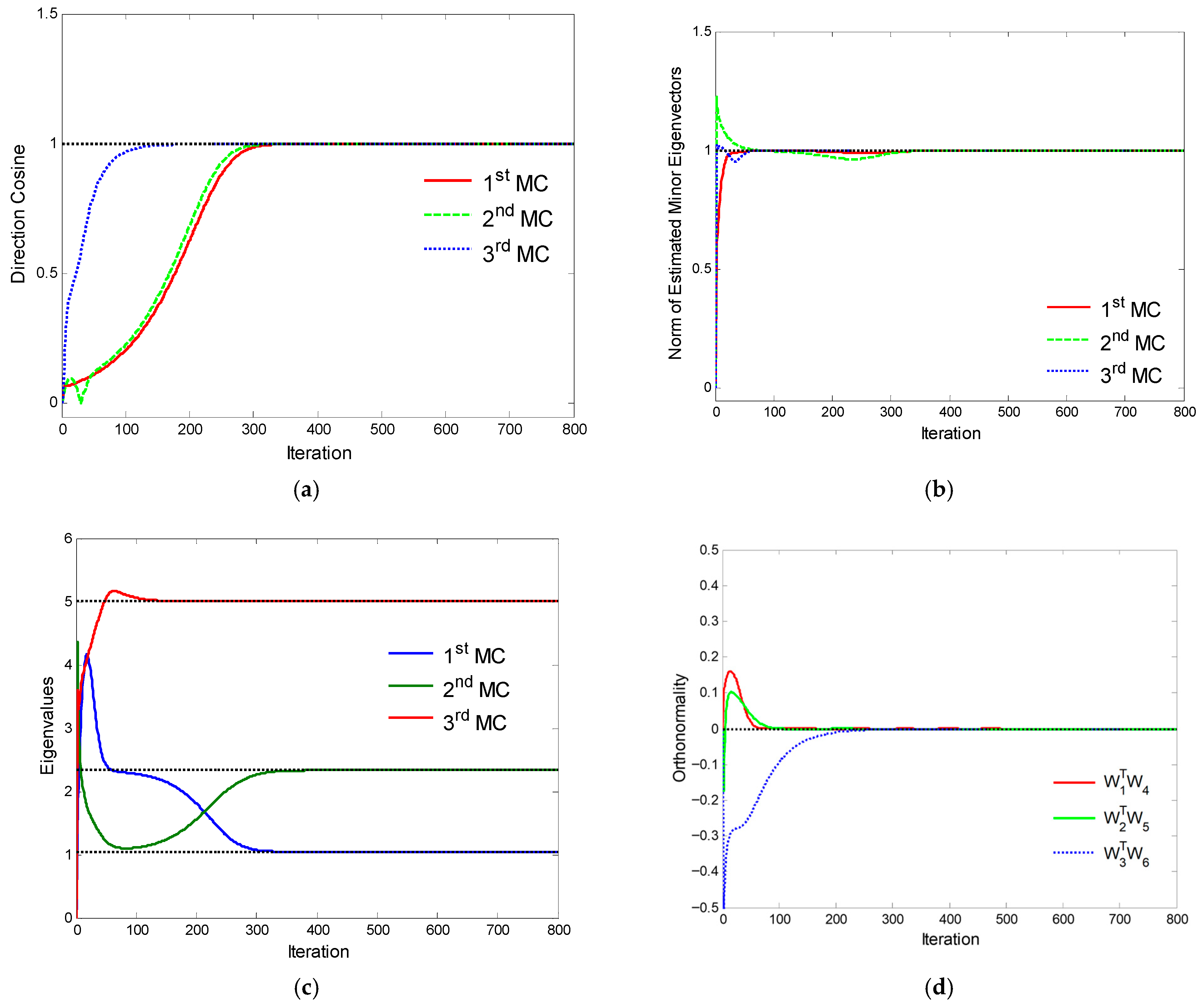
where   $e(k)$ is a Gaussian driving sequence with zero mean and unit variance. All the values of $x$ are arranged in arrays with a dimension of six ($n=6$ ). The first three ($r=3$) MCs are extracted in parallel through the proposed weighted algorithm with a random   $\mathit{W}(0)$  and   $\eta =0.02$. Then we suppose that the weighted matrix   $A=diag\{3,2,1\}$. The averaged results of 100 independent runs are shown in Figure 1.

We can see clearly in Figure 1 that multiple MCs are successfully extracted in parallel through the proposed algorithm. Both the estimated minor eigenvalues and the estimated minor eigenvectors asymptotically converge to the corresponding actual values. At the same time, the minor subspace spanned by the estimated minor eigenvectors approaches the orthogonal subspace of the principal subspace.

Example 2.

In the second example, the data were generated with the exact auto-correlation matrix   $\mathit{R}$ ,

$$\mathit{R}=\left[\begin{array}{cccccc}3.6963& 1.2644& 0.1562& 0.1171& -0.2446& -0.9896\\ 1.2644& 3.9842& 0.6116& -0.3452& 1.1380& -0.4918\\ 0.1562& 0.6116& 5.6049& 0.1870& -0.3049& 0.6375\\ 0.1171& -0.3452& 0.1870& 4.8370& 1.0312& -1.3812\\ -0.2446& 1.1380& -0.3049& 1.0312& 3.9352& 1.1647\\ -0.9896& -0.4918& 0.6375& -1.3812& 1.1647& 3.7170\end{array}\right]$$

where the eigenvalues are   $\left\{1.0520,2.3346,5.0019,5.2511,6.0117,6.1233\right\}$. The parameters are the same as with Example 1, and the results are shown in Figure 2.

5.2. Comparison with the Douglas Algorithm

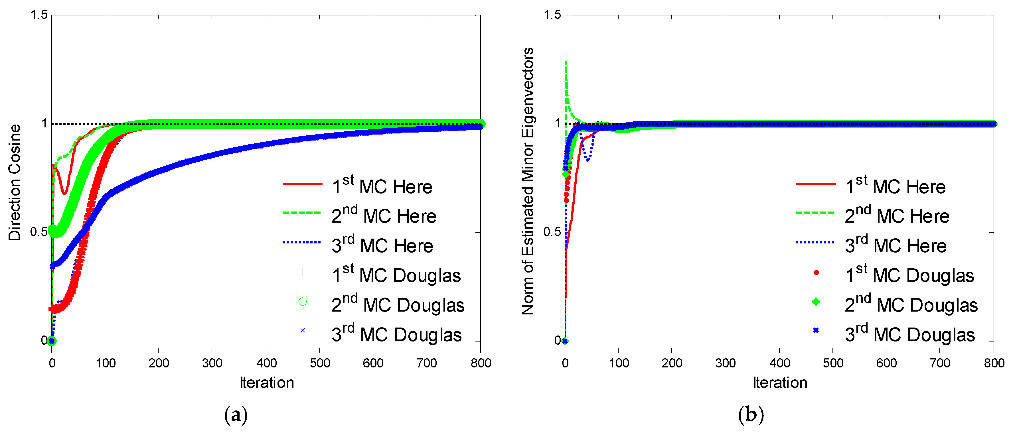
A comparison is made between the proposed weighted algorithm and the Douglas algorithm [23], which was proposed in recent years. The data are generated in a similar way to Example 1 in Section 5.1. In both algorithms, the first three ($r=3$) MCs are extracted in parallel with a random $\mathit{W}(0)$. The other initial parameters are given in

Table 1. Initial parameters of the two algorithms.

	Proposed Algorithm	Douglas’s Algorithm
Learning rate	$\eta =0.02$	$\eta =0.02$
Other parameter	A = diag ([1–3])	$\alpha =-0.1$

and the simulation results are shown in Figure 3 and

Table 2. Computation times of the two algorithms.

Method	Proposed Algorithm	Douglas’s Algorithm
Time (ms)	2.05	10.55

.

As is shown in Figure 3, MCs are successfully extracted in both algorithms with the same initial condition. However, the estimated eigenvectors in the proposed algorithm converge to the actual minor subspace faster than that in the Douglas algorithm. In Table 2, the computation time is obtained on a machine running MATLAB 2010b on Windows 11 with an Intel Core I5-1340 (1.9 GHz) processer and 16 GB memory. Since the convergence speed of the proposed algorithm is faster than that of the Douglas algorithm, this means that the proposed algorithm needs fewer iterations than that of the Douglas algorithm, so the running time of the algorithm is relatively shorter. In summary, compared with the Douglas algorithm, the proposed algorithm has simpler parameter selection and a faster convergence speed.

6. Conclusions

In this paper, we have proposed a novel adaptive algorithm for multiple MC extraction from signal vectors. We establish a dependent relation of choosing the weighted matrix based on the statistics of the input signal. Based on the Möller algorithm, we proposed the weighted Möller algorithm, which could extract the multiple MCs simultaneously. Compared with some similar algorithms, there is not extra computation for the orthonormality operations. The simulation results show that in the proposed algorithm the convergence is faster than other similar algorithms.

The advantage of the proposed algorithm is that it has no restrictions on the values of the diagonal matrix, but the proposed algorithm, the Douglas algorithm, and other algorithms are all based on the Hebbian neural network. One common problem for such algorithms is selecting the value of the learning rate. For single MC extraction algorithms, this work can be accomplished using the deterministic discrete time (DDT) method. However, the DDT method is not suitable for the subspace tracking algorithm and multiple MC extraction algorithm. Therefore, studying the range of learning factor values that ensure the stability of the algorithm has become the main direction of our subsequent work.

References

1. Zhou, C.; Gu, Y.; Fan, X.; Shi, Z.; Mao, G.; Zhang, Y.D. Direction-of-Arrival Estimation for Coprime Array via Virtual Array Interpolation. IEEE Trans. Signal Process. 2018, 66, 5956–5971. [Google Scholar] [CrossRef]
2. Mahouti, P.; Belen, A.; Tari, O.; Belen, M.A.; Karahan, S.; Koziel, S. Data-Driven Surrogate-Assisted Optimization of Metamaterial-Based Filtenna Using Deep Learning. Electronics 2023, 12, 1584. [Google Scholar] [CrossRef]
3. Baderia, K.; Kumar, A.; Agrawal, N.; Kumar, R. Minor Component Analysis Based Design of Low Pass and BandPass FIR Digital Filter Using Particle Swarm Optimization and Fractional Derivative. In Proceedings of the 2021 International Conference on Control, Automation, Power and Signal Processing (CAPS), Jabalpur, India, 10–12 December 2021; pp. 1–6. [Google Scholar]
4. Tuan, D.N.; Yamada, I. A unified convergence analysis of normalized PAST algorithms for estimating principal and minor components. Signal Process. 2013, 93, 176–184. [Google Scholar] [CrossRef]
5. Xu, L.; Oja, E.; Suen, C.Y. Modified hebbian learning for curve and surface fitting. Neural Netw. 1992, 5, 441–457. [Google Scholar] [CrossRef]
6. Huang, C.; Song, Y.; Ma, H.; Zhou, X.; Deng, W. A multiple level competitive swarm optimizer based on dual evaluation criteria and global optimization for large-scale optimization problem. Inf. Sci. 2025, 708, 122068. [Google Scholar] [CrossRef]
7. Ma, Y.; Cheng, J. A novel joint denoising method for gear fault diagnosis with improved quaternion singular value decomposition. Measurement 2024, 226, 114165. [Google Scholar] [CrossRef]
8. Yi, K.; Cai, C.; Tang, W.; Dai, X.; Wang, F.; Wen, F. A Rolling Bearing Fault Feature Extraction Algorithm Based on IPOA-VMD and MOMEDA. Sensors 2023, 23, 8620. [Google Scholar] [CrossRef]
9. Chung, D.; Jeong, B. Analyzing Russia–Ukraine War Patterns Based on Lanchester Model Using SINDy Algorithm. Mathematics 2024, 12, 851. [Google Scholar] [CrossRef]
10. Wang, Z.; Li, S.; Xuan, J.; Shi, T. Biologically Inspired Compound Defect Detection Using a Spiking Neural Network With Continuous Time–Frequency Gradients. Adv. Eng. Inform. 2025, 65, 103–132. [Google Scholar] [CrossRef]
11. Zhang, X.; Li, Y.; Feng, X.; Hua, J.; Yue, D.; Wang, J. Application of Multiple-Optimization Filtering Algorithm in Remote Sensing Image Denoising. Sensors 2023, 23, 7813. [Google Scholar] [CrossRef] [PubMed]
12. Giuliani, A.; Vici, A. On the (Apparently) Paradoxical Role of Noise in the Recognition of Signal Character of Minor Principal Components. Stats 2024, 7, 54–64. [Google Scholar] [CrossRef]
13. Xuan, J.; Wang, Z.; Li, S.; Gao, A.; Wang, C.; Shi, T. Measuring compound defect of bearing by wavelet gradient integrated spiking neural network. Measurement 2023, 223, 10. [Google Scholar] [CrossRef]
14. Ma, Q.; Sun, Y.; Wan, S.; Gu, Y.; Bai, Y.; Mu, J. An ENSO Prediction Model Based on Backtracking Multiple Initial Values: Ordinary Differential Equations–Memory Kernel Function. Remote Sens. 2023, 15, 3767. [Google Scholar] [CrossRef]
15. Mathew, G.; Reddy, V. Orthogonal eigensubspace estimation using neural networks. IEEE Trans. Signal Process. 1994, 42, 1803–1811. [Google Scholar] [CrossRef]
16. Rahmat, F.; Zulkafli, Z.; Ishak, A.J.; Abdulrahman, R.Z.; Stercke, S.D.; Buytaert, W.; Tahir, W.; Abrahman, J.; Ibrahim, S.; Ismail, M. Supervised feature selection using principal component analysis. Knowl. Inf. Syst. 2024, 66, 1955–1995. [Google Scholar] [CrossRef]
17. Dai, H. Application of PCA Numalgorithm in Remote Sensing Image Processing. Mod. Electron. Technol. 2023, 7, 17–21. [Google Scholar] [CrossRef]
18. Gao, Y. Adaptive Generalized Eigenvector Estimating Algorithm for Hermitian Matrix Pencil. IEEE/CAA J. Autom. Sin. 2022, 9, 1967–1979. [Google Scholar] [CrossRef]
19. Cai, H.; Kaloorazi, M.F.; Chen, J.; Chen, W.; Richard, C. Online dominant generalized eigenvectors extraction via a randomized method. In Proceedings of the 28th European Signal Processing Conference, Amsterdam, The Netherlands, 18–21 January 2021. [Google Scholar]
20. Möller, R. A self-stabilizing learning rule for minor component analysis. Int. J. Neural Syst. 2004, 14, 1–8. [Google Scholar] [CrossRef] [PubMed]
21. Peng, D.; Zhang, Y.; Xiang, Y.; Zhang, H. A globally convergent MC algorithm with an adaptive learning rate. IEEE Trans. Neural Netw. Learn. Syst. 2012, 23, 359–365. [Google Scholar] [CrossRef] [PubMed]
22. Tanaka, T. Generalized weighted rules for principal components tracking. IEEE Trans. Signal Process. 2005, 53, 1243–1253. [Google Scholar] [CrossRef]
23. Jankovic, M.V.; Reljin, B. A new minor component analysis method based on Douglas-Kung-Amari minor subspace analysis method. IEEE Signal Process. Lett. 2005, 12, 859–862. [Google Scholar] [CrossRef]
24. Ouyang, S.; Bao, Z. Fast Principal Component Extraction by a Weighted Information Criterion. IEEE Trans. Signal Process. 2002, 50, 1994–2002. [Google Scholar] [CrossRef]
25. Du, B.; Kong, X.; Feng, X. Generalized principal component analysis-based subspace decomposition of fault deviations and its application to fault reconstruction. IEEE Access 2020, 8, 34177–34186. [Google Scholar] [CrossRef]
26. Kong, X.; Hu, C.; Duan, Z. Principal Component Analysis Networks and Algorithms; Springer: Beijing, China, 2017. [Google Scholar]
27. Tan, K.K.; Lv, J.; Zhang, Y.; Huang, S. Adaptive multiple minor directions extraction in parallel using a PCA neural network. Theor. Comput. Sci. 2010, 411, 4200–4215. [Google Scholar] [CrossRef]
28. Jou, Y.-D.; Chen, F.-K. Design of equiripple FIR digital differentiators using neural weighted least-squares algorithm. In Proceedings of the 2011 8th International Conference on Information, Communications & Signal Processing, Singapore, 13–16 December 2011; pp. 1–5. [Google Scholar]
29. Hasan, M.A. Diagonally weighted and shifted criteria for minor and principal component extraction. In Proceedings of the IEEE International Joint Conference on Neural Networks, IJCNN ‘05, Montreal, QC, Canada, 31 July–4 August 2005; Volume 1252, pp. 1251–1256. [Google Scholar]
30. Jou, Y.-D.; Chen, F.-K.; Sun, C.-M. Neural weighted least-squares design of FIR higher-order digital differentiators. In Proceedings of the 2009 16th International Conference on Digital Signal Processing, Santorini, Greece, 5–7 July 2009; pp. 1–5. [Google Scholar]
31. Du, K.-L.; Swamy, M.N. Neural Networks and Statistical Learning, 1st ed.; Springer: London, UK, 2019. [Google Scholar]
32. Qiu, J.; Wang, H.; Lu, J.; Zhang, B. Neural network implementations for PCA and its extensions. ISRN Artif. Intell. 2012, 2012, 847305. [Google Scholar] [CrossRef]
Figure 1. Simulation results for the transient behavior of the proposed algorithm for Example 1. (a) Direction cosine curves. (b) Norm of the estimated minor eigenvectors. (c) Estimated minor eigenvalues. (d) Orthogonality of the estimated MCs.
Electronics 14 04073 g001
Figure 2. Simulation results for the transient behavior of the proposed algorithm for Example 2. (a) Direction cosine curves. (b) Norm of the estimated minor eigenvectors. (c) Estimated minor eigenvalues. (d) Orthogonality of the estimated MCs.
Electronics 14 04073 g002
Figure 3. Simulation results for comparison between the proposed algorithm and the Douglas algorithm. (a) Direction cosine curves. (b) Norm of the estimated minor eigenvectors.
Electronics 14 04073 g003