Sales Forecasting for New Products Using Homogeneity-Based Clustering and Ensemble Method

Abstract

Accurate sales forecasting for new products is critical in industries characterized by intense competition, rapid innovation, and short product life cycles, such as the smartphone market. This study proposes a data-driven framework that enhances prediction accuracy by combining homogeneity-based clustering with an ensemble learning approach. Unlike traditional methods that depend on product-specific attributes, our approach utilizes historical sales data from similar products, overcoming attribute dependency. Using K-means clustering, the training data are segmented into homogeneous groups, and tailored ensemble forecasting models are developed for each cluster by combining five machine learning models: Random Forest, Extra Tree, XGBoost, LightGBM, and TabNet. When tested on South Korean smartphone sales data, the framework achieves superior performance, with the optimal ensemble model using four clusters delivering an MAPE of 8.3309% and an RMSPE of 7.8360%, significantly outperforming traditional single-cluster models. These findings demonstrate the effectiveness of leveraging data homogeneity and ensemble methods, offering a scalable and adaptable solution for accurate sales forecasting of new products.

1. Introduction

The current economic landscape is marked by shorter product life cycles, rapid innovation, and expansion in product lines, underscoring the need for precise sales forecasting [1,2]. Accurate forecasting of new product sales is crucial to maintaining a company’s competitive edge, as forecasting errors can lead to financial issues, including overstocking or missed sales opportunities [3]. The increasing diversity of products, along with the inherent complexities of prediction, further complicates the process of sales forecasting. Traditional qualitative methods rely heavily on industry expert insights but are often swayed by biased and unpredictable market trends [4,5]. Despite advancements in quantitative techniques, achieving reliable sales forecasts for new products remains a challenge. Prior studies have frequently utilized historical sales data and attributes from comparable products to forecast new product sales [6,7]. However, these approaches may encounter issues with uncertainty and accuracy, particularly when a new product possesses unique features or when there are no directly comparable products.

To address these challenges, we propose a novel methodology that leverages past sales data from similar products without relying on specific product attributes. The primary aim of this research is to develop a practical and accurate sales forecasting framework for new products. Specifically, our objective is to enhance prediction accuracy and reduce uncertainty in forecasting by using homogeneity-based clustering to group products with similar sales trends. By constructing training datasets with homogeneous patterns, our framework ensures improved model performance, as this approach has been shown to enhance the accuracy of machine learning and deep learning techniques [8,9,10]. Furthermore, we employ ensemble methods to improve robustness and generalization, addressing the complexities of dynamic markets and diverse product portfolios. Our methodology offers a scalable solution that adapts to market volatility, enabling industries to make data-driven decisions with greater confidence.

Our study defines the sales forecast cycle for a product as weekly, as this interval effectively captures market responses and is practical [11]. However, weekly sales data are often less extensive than daily sales data. To address this, we select machine learning models, which tend to be less sensitive to data volume compared to deep learning models that generally require larger datasets, which may not be available for new products [12]. Among machine learning models, we focus on tree-based algorithms due to their reliable performance with smaller datasets [13,14,15]. Additionally, we employ the soft-voting ensemble method, which combines multiple machine learning models to enhance prediction accuracy and generalization capabilities [16,17]. We demonstrate the efficacy of our approach using real-world weekly smartphone sales data. Our results confirm that our model is practical and significantly improves the accuracy and reliability of sales forecasts for new products.

This paper is structured as follows: Section 2 reviews the existing literature, providing the foundation for our research. Section 3 outlines our research methodology, including the clustering algorithms and ensemble method we employed. Section 4 details data collection, model construction, empirical results, and evaluates our model’s performance. The Section 5 summarizes our findings and suggests directions for future research.

2. Literature Review

Numerous studies have explored various approaches to improve the accuracy of new product sales forecasting. Traditional statistical models have been widely employed for this purpose. For instance, one study predicted Bass model parameters using product attribute and diffusion data, improving forecasting accuracy through a machine learning-based ensemble model, with significant performance improvements demonstrated in the case of 3D TV sales [18]. Another study leveraged the correlation between short-term and long-term cumulative sales of similar product groups to predict long-term sales based on initial sales data of newly launched products, achieving practical accuracy in cases of books and electronic devices in Japan [19]. Additionally, ARIMAX models have shown 21–24% lower forecast errors compared to neural networks for clean data, although neural networks exhibited greater robustness in noisy datasets, highlighting trade-offs between traditional and advanced methods [20].

Recent advancements in data-driven approaches, particularly machine learning and deep learning, have further enhanced forecasting accuracy. Clustering-based techniques, such as K-means and GHSOM combined with models like SVR and ELM, achieved a 15–20% improvement in prediction accuracy by analyzing similar product attributes, including data patterns and features. This approach proved effective in the computer retail industry [7]. Another study enhanced sales forecasting in the Korean smartphone market by leveraging product attributes and sales histories of similar products. This study utilized various algorithms, including Ridge, Lasso, SVM, Random Forest, eXtreme Gradient Boosting (XGBoost), CatBoost, and others, with Random Forest demonstrating the highest accuracy [6]. Additionally, the DemandForest method integrated K-means clustering with Random Forest and Quantile Regression Forest, proving effective for product feature analysis and inventory management [21]. Advanced data-driven methods have also been employed to capture non-linear patterns and short-term fluctuations. For instance, combining fuzzy clustering with LSTM achieved a 15–30% improvement in forecasting accuracy compared to traditional Bass models, effectively modeling seasonality and sales cycles [22]. Multi-modal approaches have also shown promise; one study combined product attributes (images, categories) with external factors (discounts, events, weather), achieving an over 15% improvement in forecasting accuracy compared to k-NN-based methods, validated using fashion retail data [23]. Furthermore, a study used sales data from 800 products over 49 weeks to predict fourth-week sales based on the previous three weeks using a recurrent neural network (RNN), achieving high accuracy with an RMSE of 0.039 and effectively capturing product sales trends [24]. Machine learning algorithms like XGBoost, Light Gradient Boosting Machine (LightGBM), and CatBoost have also been utilized to predict new product demand based on attributes such as price, category, and textual descriptions, achieving a 15–20% improvement in accuracy compared to traditional statistical methods [25]. Another study proposed integrating a product differentiation index with prior demand data to model the non-linear relationship between market demand and product differentiation. This approach significantly improved forecasting accuracy in the automotive industry [26]. A study leverages the characteristics of similar products to analyze customer preferences and forecast sales for new products, demonstrating that the proposed machine learning-based model reduces the mean absolute percentage error by 15% and improves the $R^2$ value to 0.92 compared to existing models [27].

Existing research has applied various data-driven methods to forecast sales of new products, often relying on attributes of similar existing products. However, these approaches face significant challenges when predicting sales for products with unique features or those lacking comparable precedents—issues that are especially pronounced in rapidly evolving markets. To overcome these limitations, we propose a methodology that shifts from attribute-based analysis to identifying homogeneous sales trends. Using K-means clustering, we group products based on similar sales trajectories, enabling the segmentation of homogeneous training datasets that enhance machine learning performance by focusing on clearer and more consistent patterns. Our framework also incorporates a soft-voting ensemble method, combining models such as Random Forest, Extra Tree, XGBoost, LightGBM, and Tabular Attention Network (TabNet) to improve prediction accuracy and reliability. Testing on South Korean smartphone sales data demonstrated the robustness of this approach, delivering accurate and reliable forecasts for new products regardless of their unique attributes. This methodology effectively addresses the limitations of existing methods and provides a practical solution for improving sales forecasting in dynamic markets.

3. Methodology

In this section, we present our proposed framework for accurately forecasting sales of new products. We elaborate on the predictor variables, clustering algorithm, and ensemble method used in this study.

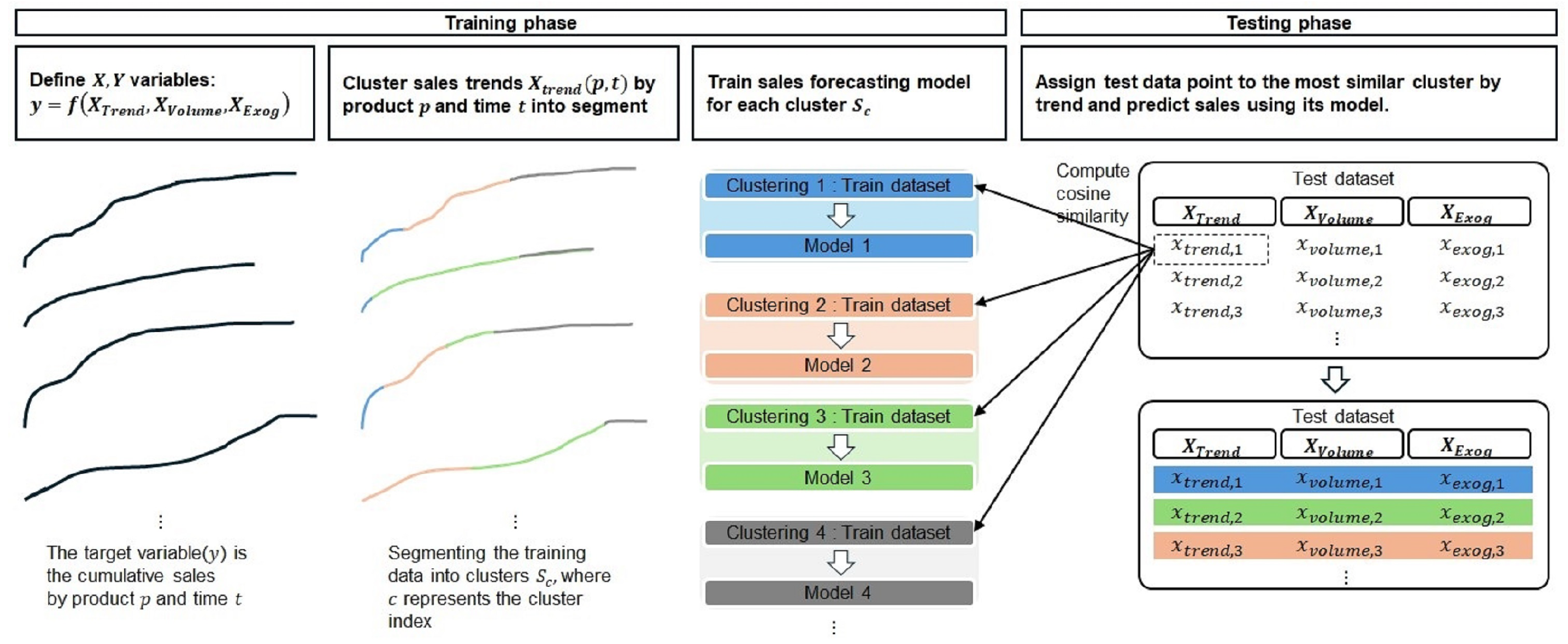
3.1. Proposed Framework

Our proposed sales forecasting model for new products is an ensemble model based on data homogeneity. The methodology consists of two stages: the training phase and the testing phase. Figure 1 illustrates these stages for predicting new product sales. In the left panel of Figure 1, the curves represent the cumulative sales volume (y) of different products (p) over time (t), where the x-axis corresponds to time (t) in weeks, and the y-axis corresponds to cumulative sales volume (y). These curves highlight sales trends, which are used to cluster products with similar trajectories for more accurate forecasting.

In the training phase, the predictor set $X_k$ includes variables related to sales trends, sales volume, and exogenous factors, where k represents an index identifying specific predictors. These predictors are categorized into three main types: sales trend-related predictors ($X_{\mathrm{trend}}$), sales volume-related predictors ($X_{\mathrm{volume}}$), and exogenous variables ($X_{\mathrm{exog}}$), forming the matrix $X=[X_{\mathrm{trend}},X_{\mathrm{volume}},X_{\mathrm{exog}}]$. The target variable y represents the cumulative sales for each product at a given time period, serving as the dependent variable in the model.

Data are clustered based on similar sales trends using only the sales trend-related predictors ($X_{\mathrm{trend}}$). The clustering does not directly depend on the product p or time t; instead, it is determined solely by the similarity of $X_{\mathrm{trend}}(p,t)$ values. As a result, each cluster c can include data points from different products and time periods that share similar sales trends. The clustering function is defined as follows:

$$c=f(p,t)=arg\underset{c}{min}∥X_{\mathrm{trend}}(p,t)-{\mu }_c∥$$

(1)

where $X_{\mathrm{trend}}(p,t)$ represents the vector of sales trend-related predictors for product p at time t, and ${\mu }_c$ is the centroid of cluster c. Once clustering is complete, the training dataset is segmented into subsets $S_c$, where each subset corresponds to a cluster c, grouping data points with similar sales trends. The centroid ${\mu }_c$ is a vector representing the mean of the trend-related predictors $X_{\mathrm{trend}}$ within cluster c, with its dimension matching the number of features in $X_{\mathrm{trend}}$. The cluster $S_c$ is a set of tuples, where each tuple contains the predictor variables $X_{(p,t)}$ and the corresponding target variable $y_{(p,t)}$, such that $S_c=\{(X_{(p,t)},y_{(p,t)})\mid (p,t)\in \mathrm{Cluster}c\}$. This structure ensures that data points within the same cluster share similar sales trends, enhancing model homogeneity and accuracy.

For each data segment, an ensemble model $f_c\left(X\right)$ is trained, representing the predictive model for cluster c. The model training for each cluster is as follows:

$$f_c\left(X\right)=arg\underset{\theta }{min}\sum _{(p,t)\in S_c}l(y_{(p,t)},g(X_{(p,t)};\theta ))$$

(2)

where l is the loss function, $y_{(p,t)}$ represents actual sales, $X_{(p,t)}$ are the predictors, and $g(X_{(p,t)};\theta )$ is the model parameterized by $\theta$. This approach enhances predictive accuracy by targeting segments with homogeneous patterns.

In the testing phase, the objective is to identify the cluster whose trend pattern closely aligns with a given test data point.

Each test data point, denoted by z, belongs to the test dataset ${\mathbf{X}}^{\mathrm{test}}$. To determine the best match, cosine similarity is computed between the trend-related predictors of z, $X_{\mathrm{trend}}\left(z\right)$, and the centroid ${\mu }_c$ of each cluster. The similarity is calculated as follows:

$$\mathrm{sim}(X_{\mathrm{trend}}\left(z\right),{\mu }_c)={\displaystyle \frac{X_{\mathrm{trend}}\left(z\right)·{\mu }_c}{\parallel X_{\mathrm{trend}}\left(z\right)\parallel \parallel {\mu }_c\parallel }}.$$

(3)

The cluster $c^{*}$ that achieves the highest cosine similarity is selected as the most similar cluster. Using the predictive model $f_{c^{*}}\left(X\right)=g(X;{\theta }_c^{*})$, where ${\theta }_c^{*}$ minimizes the loss function $l(y,g(X;{\theta }_c))$ during training, the sales volume for the test data point z is predicted as follows:

$$\widehat{y}\left(z\right)=f_{c^{*}}\left(X\left(z\right)\right).$$

(4)

The loss function $l\left(\right)$ is solely used during training to optimize ${\theta }_c$ and does not play a role in the prediction process during testing.

The described procedure can be formulated as shown in Algorithm 1.

Algorithm 1: New product sales forecasting with data homogeneity clustering.

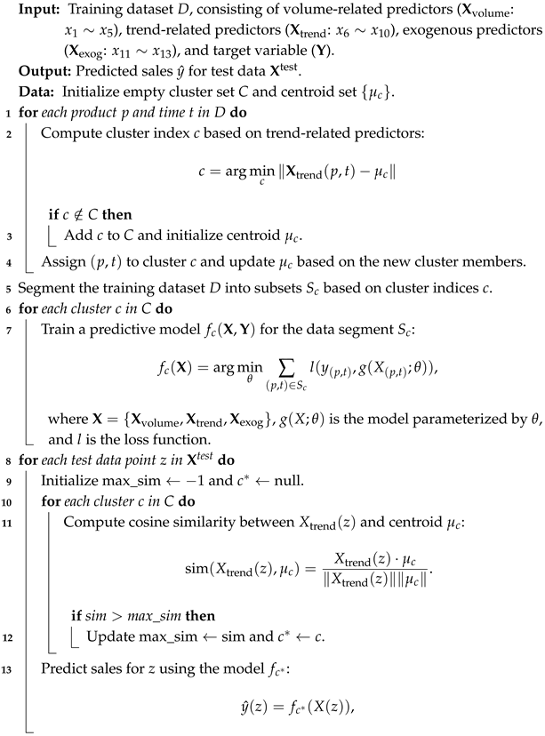3.2. Predictor Variables

In our study, we define the target variable y as the cumulative weekly sales volume for the product. To stabilize variance in weekly sales data, we apply a log transformation. This transformation helps reduce skewness and handle outliers, thereby increasing the reliability of our forecasts [28,29]. Finally, our forecasting model uses three types of independent variables: sales volume-related variables, sales trend-related variables, and exogenous variables derived from Google Trends. The three-week time window ($t-3\sim t-1$) is selected to capture recent sales trends effectively while avoiding the noise associated with outdated data [30,31,32]. This choice balances the need for sufficient historical context with the relevance of recent patterns, aligning with best practices in demand forecasting research. Since our model predicts weekly sales, let t represent the current week for which the forecast is being made. The variables are defined as follows:

3.2.1. Sales Volume-Related Variables ($x_1$ to $x_5$)

• $x_1$: Cumulative sales for the previous week ($t-1$);
• $x_2$: Cumulative sales for the week before last ($t-2$);
• $x_3$: Cumulative sales for three weeks ago ($t-3$);
• $x_4$: Moving average of cumulative sales over the last two weeks ($t-1$ and $t-2$);
• $x_5$: Moving average of cumulative sales over the last three weeks ($t-1$, $t-2$, and $t-3$).

These variables are crucial for analyzing past performance and predicting future trends. Cumulative and moving average sales data provide strong indicators of ongoing sales patterns and potential future performance [2,33].

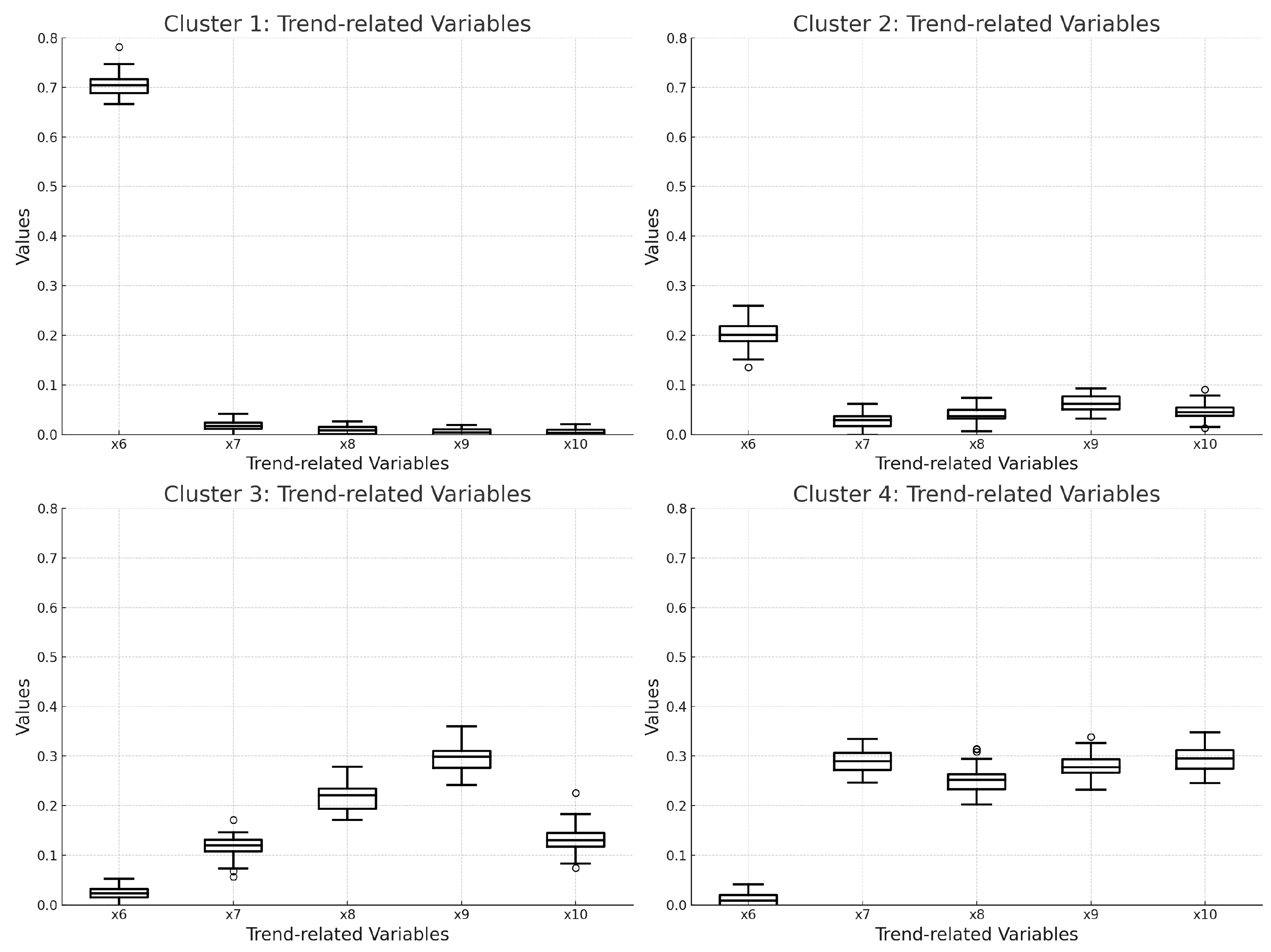
3.2.2. Sales Trend-Related Variables ($x_6$ to $x_{10}$)

• $x_6$: Number of weeks since product launch;
• $x_7$: Change rate between cumulative sales for the previous week ($t-1$) and the week before last ($t-2$);
• $x_8$: Change rate between cumulative sales for the previous week ($t-1$) and three weeks prior ($t-3$);
• $x_9$: Moving average of the change rate between cumulative sales for the previous week ($t-1$) and the week before last ($t-2$);
• $x_{10}$: Moving average of the change rate between cumulative sales for the previous week ($t-1$) and three weeks prior ($t-3$).

These variables are essential for understanding sales trends over time, which is critical for accurate forecasting. Analyzing metrics like the number of weeks since product launch, weekly change rates, and moving averages of these changes helps capture the dynamics of sales growth and decline [34,35,36].

3.2.3. Exogenous Variables ($x_{11}$ to $x_{13}$)

• $x_{11}$: Google Trends score for the previous week ($t-1$);
• $x_{12}$: Google Trends score for the week before last ($t-2$);
• $x_{13}$: Google Trends score for three weeks ago ($t-3$).

These variables help reduce prediction errors by reflecting customer interest and market trends. Google Trends data have been validated in multiple studies as a reliable indicator of consumer interest and market demand [33,36,37].

3.3. K-Means Clustering Algorithm and Ensemble Method

This section explains the K-means clustering algorithm and the ensemble method used in our study. First, we apply K-means clustering to segment the training data based on trend variables. Then, we develop a sales forecasting model for new products using soft voting, an ensemble method that combines five different machine learning algorithms.

3.3.1. K-Means Clustering

The K-means algorithm is used to cluster data with similar characteristics. It is straightforward and effective, as it segments the dataset into clusters to minimize variance within each cluster and improve pattern recognition. This method is well suited for identifying patterns and extracting features from diverse datasets [38,39].

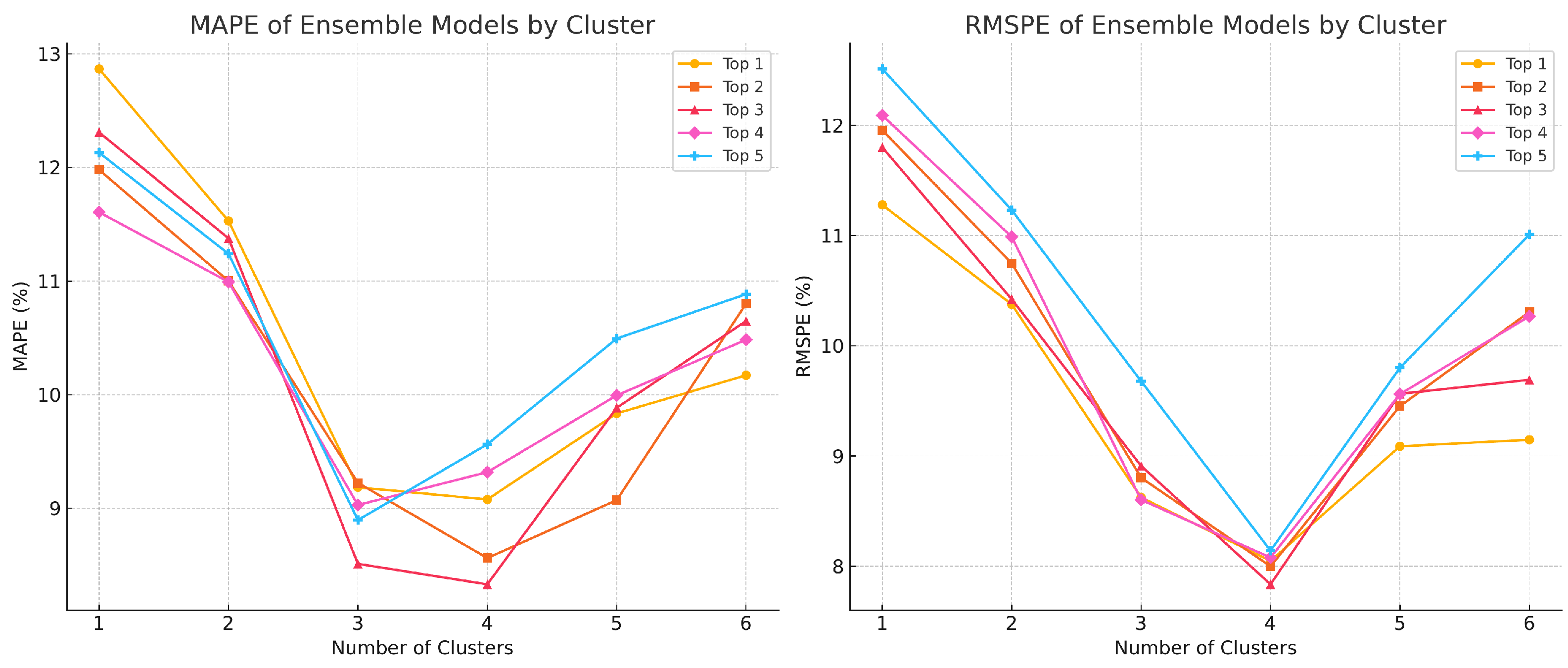
3.3.2. Ensemble Method

To enhance prediction accuracy, minimize errors, handle diverse data characteristics, and avoid overfitting, we use an ensemble method. This approach leverages the strengths of multiple algorithms through a soft voting mechanism, where predictions from each model are averaged to improve reliability and generalization ability [40]. The final prediction in the soft voting ensemble is calculated as follows:

$$\widehat{y}={\displaystyle \frac{1}{N}}\sum _{i=1}^N{\widehat{y}}_i,$$

(5)

where $\widehat{y}$ is the final predicted sales value, N is the number of models in the ensemble, and ${\widehat{y}}_i$ represents the sales prediction from the i-th model. Each model in the ensemble uses the predictor variables $X_{\mathrm{volume}},X_{\mathrm{trend}},X_{\mathrm{exog}}$, which correspond to sales volume, sales trends, and exogenous factors, respectively, as inputs.

To further optimize prediction accuracy, we construct soft voting ensembles using the Top N machine learning models based on their performance. The selection of models in the Top N ensemble dynamically adjusts depending on the total number of available models, ensuring that only the best-performing models contribute to the final prediction. This adaptive approach enhances the flexibility and effectiveness of the ensemble method, allowing it to consistently leverage the strengths of the most reliable models.

The ensemble consists of a combination of the following five machine learning algorithms:

Random Forest improves prediction accuracy and mitigates overfitting by aggregating forecasts from multiple decision trees. It benefits from randomness in tree generation and data bootstrapping, which increases tree diversity and reduces model variance [41,42]. The Random Forest model uses $X_{\mathrm{volume}},X_{\mathrm{trend}},X_{\mathrm{exog}}$ as input variables to generate predictions, effectively capturing both historical sales patterns and exogenous influences.

Extra Tree introduces extra randomness in node splits and uses the entire dataset for tree development. This method reduces model variance and enhances robustness against overfitting, particularly in complex scenarios [43]. The Extra Tree model also leverages $X_{\mathrm{volume}},X_{\mathrm{trend}},\mathrm{and}{X}_{\mathrm{exog}}$ to construct decision trees that identify patterns in sales trends and exogenous factors.

LightGBM is a gradient boosting framework known for its computational efficiency. It employs techniques such as Gradient-Based One-Side Sampling and Exclusive Feature Bundling to expedite training and reduce data dimensionality [44]. The iterative update mechanism is represented as follows:

$$F_{t+1}\left(X\right)=F_t\left(X\right)+\eta \sum _{i=1}^N{\gamma }_i{h}_i\left(X\right),$$

(6)

where $F_t\left(X\right)$ is the model at iteration t, $\eta$ signifies the learning rate, and ${\gamma }_i$ are the gradients of the loss function with respect to the predictions $h_i\left(X\right)$ at iteration t. In this context, X refers to $X_{\mathrm{volume}},X_{\mathrm{trend}},X_{\mathrm{exog}}$, ensuring that the LightGBM model utilizes comprehensive information about sales dynamics and exogenous factors.

XGBoost, eXtreme Gradient Boosting, optimizes both computational speed and model performance by employing a regularized learning framework. This framework adds a regularization term to the objective function to control the model’s complexity, thus helping to reduce overfitting [45]. The general form of the objective function is the following:

$$\mathrm{Obj}=\sum _{i=1}^{n}L(y_i,{\widehat{y}}_i)+\sum _{k=1}^K\Omega \left(f_k\right),$$

(7)

where L is a differentiable loss function measuring the difference between the predicted ${\widehat{y}}_i$ and actual $y_i$ outcomes, and $\Omega$ penalizes the complexity of the model. The variables n and k are defined as follows: n represents the total number of observations, and k represents the index of features or components. The XGBoost model processes $X_{\mathrm{volume}},X_{\mathrm{trend}},\mathrm{and}{X}_{\mathrm{exog}}$ as inputs to optimize predictions by balancing model complexity and generalization.

TabNet, abbreviated for Tabular Attention Network, dynamically selects which features to reason from at each decision iteration, thereby focusing computational resources on the most informative parts of the data [46]. This process allows TabNet to achieve both high interpretability and performance:

$$\mathrm{Output}=\sum _{\mathrm{iteration}=1}^{\mathrm{Iterations}}{M}_{\mathrm{iteration}}·D_{\mathrm{iteration}}\left(X\right),$$

(8)

where $M_{\mathrm{iteration}}$ and $D_{\mathrm{iteration}}\left(X\right)$ represent the mask and decision function at each iteration, respectively. The input X corresponds to $X_{\mathrm{volume}},X_{\mathrm{trend}},X_{\mathrm{exog}}$, ensuring that TabNet dynamically prioritizes the most relevant predictors for each sales scenario.

4. Experiments and Results

This section details data collection and preprocessing, metrics for evaluating and validating the forecasting model, hyperparameter optimization strategies during model development, and the final results for test datasets. Specifically, we analyze performance differences by considering two factors: data homogeneity and the use of ensemble method.

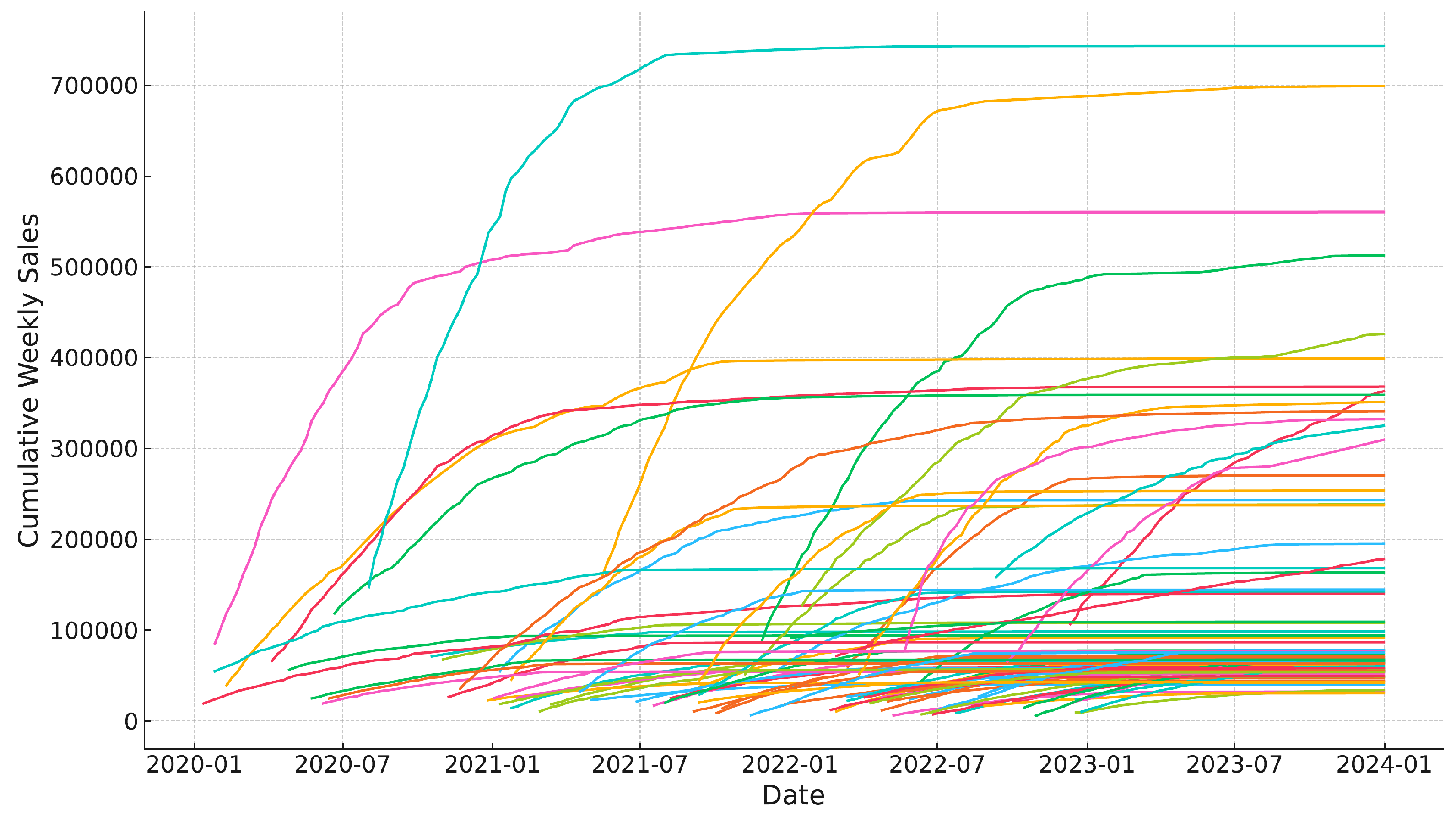
4.1. Data Collection and Preprocessing

We collected weekly cumulative sales data for 79 smartphone products in South Korea from 1 January 2020 to 31 December 2023. These data were provided by one of the three major mobile carriers in South Korea. The dataset consists of 10,012 data points, focusing on models released after 1 January 2020. Figure 2 illustrates the cumulative weekly sales for each product. Each product has a different launch date, so the starting point of sales varies, as does the cumulative sales growth rate across products.

The data collection periods for these products varied widely, ranging from a minimum of 50 weeks to a maximum of 190 weeks. A statistical summary of the weekly cumulative sales data is provided in

Table 1. Statistics on weekly cumulative sales for each product.

Data Count	Mean	Median	Min	Max
10,012	92,281.12	55,698	44	73,813

, and a summary of product-specific collection periods is provided in

Table 2. Statistics on duration of weekly sales for each product.

Number of Products	Mean	Median	Min	Max
79	107.57	109	50	190

.

Additionally, we collected Google Trends values by searching each product name on the Google Trends website (https://trends.google.co.kr/trends/ (accessed on 8 October 2024)) to use as an exogenous variable. The data were retrieved by inputting the exact product names as keywords into the platform, ensuring consistency across all products. Google Trends provides normalized interest scores ranging from 0 to 100, where 100 represents the peak search interest within the specified timeframe and region. The weekly search data for each product were then aligned with its sales data to maintain temporal consistency. This alignment ensured that the exogenous variable accurately reflected public interest during the corresponding sales periods.

During preprocessing, we applied min–max normalization to the x variables to adjust for scale discrepancies among the predictors for the y target variable. This method scales the predictors between 0 and 1, eliminating the influence of size discrepancies [47,48]. The min–max normalization is defined as follows:

$$x^{\prime }={\displaystyle \frac{x-min\left(x\right)}{max\left(x\right)-min\left(x\right)}}$$

(9)

where x represents the original value, $min\left(x\right)$ and $max\left(x\right)$ are the minimum and maximum values of x, and $x^{\prime }$ is the normalized value.

4.2. Evaluation Procedures and Metrics

We evaluated our model using nested cross-validation, a robust method that separates hyperparameter tuning from performance evaluation to prevent data leakage and provide an unbiased estimate of model generalization [49]. To fully utilize our dataset of 79 products and leverage the advantages of Leave-One-Out Cross-Validation (LOOCV), such as maximizing data utilization and reducing bias from specific data splits [50,51], we extended this framework to nested LOOCV. In this approach, each product is sequentially designated as the test set in the outer loop, while the remaining products constitute the training set. The training set is further split within each iteration for hyperparameter tuning, ensuring that hyperparameters are optimized exclusively on the training data and never exposed to the outer test set.

To assess model accuracy, we employed two metrics: Mean Absolute Percentage Error (MAPE) and Root Mean Square Percentage Error (RMSPE). Both metrics are intuitive, scale-independent, and widely used across various studies [52,53]. MAPE measures the average absolute percentage difference between predicted and actual values, making it effective for detecting subtle prediction errors. Conversely, RMSPE emphasizes larger errors or outliers by calculating the square root of the mean squared percentage errors. Given their unique strengths, a comprehensive evaluation using both metrics is warranted [54,55], which we apply in our study. The formulas for MAPE and RMSPE are as follows:

$$\mathrm{MAPE}={\displaystyle \frac{1}{n}}\sum _{i=1}^n\left|{\displaystyle \frac{y_i-{\widehat{y}}_i}{y_i}}\right|\times 100$$

(10)

$$\mathrm{RMSPE}=\sqrt{{\displaystyle \frac{1}{n}}\sum _{i=1}^n{\displaystyle \frac{{(y_i-{\widehat{y}}_i)}^2}{y_i^2}}\times 100}$$

(11)

where $y_i$ is the actual value, ${\widehat{y}}_i$ is the predicted value, and n is the number of observations.

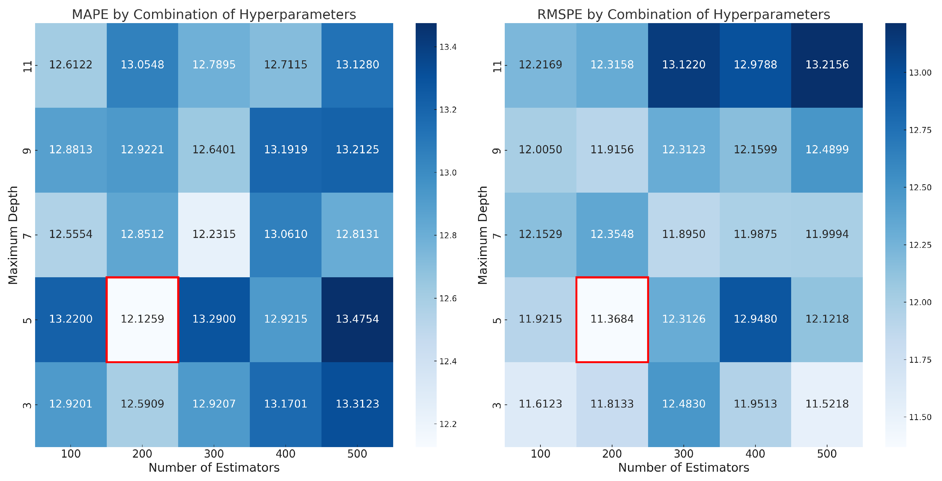
4.3. Model Development and Optimization

In this study, we developed an ensemble model using soft voting, combining five different machine learning algorithms to predict sales volume. Effective hyperparameter tuning during the training phase is essential for enhancing prediction accuracy [56,57]. This involves adjusting each model’s hyperparameters for each iteration of nested LOOCV. For instance, in the first LOOCV iteration, product $p=1$ is used as the test data, while products $p=2$ to $p=79$ form the training set. The training set is further divided iteratively, with each product sequentially designated as validation data while the remaining products are used for training. Hyperparameter tuning is conducted via a comprehensive grid search using the inner validation data, ensuring unbiased optimization and robust performance evaluation.

For tree-based models, such as Random Forest, LightGBM, XGBoost, and Extra Tree, tuning parameters like the number of estimators and maximum depth significantly impact performance [58,59,60,61]. In our study, we identified the optimal values for these hyperparameters. For the TabNet model, we optimized key hyperparameters like maximum epochs, batch size, and virtual batch size, as they considerably affect performance [62,63].

To enhance overall model capabilities, we tested various configurations to identify the optimal settings. For the tree-based models, two key hyperparameters were considered:

• Number of Estimators: This indicates the number of trees built in the model, with candidate values of 100, 200, 300, 400, and 500.
• Maximum Depth: This sets the maximum depth each tree can achieve, tested with values of 3, 5, 7, 9, and 11.

For the TabNet model, three key hyperparameters were tested:

• Maximum Epochs: This defines the upper limit of training cycles, tested with values of 40, 60, 80, 100, and 200.
• Batch Size: This is the number of examples processed in each batch, with options of 128, 256, 512, 1024, and 2048.
• Virtual Batch Size: This size is used for “Ghost Batch Normalization”, with tested sizes of 32, 64, 128, 256, and 512.

To illustrate the hyperparameter optimization process, we examine a Random Forest model applied to a single cluster. This example provides a step-by-step demonstration of how hyperparameters are systematically evaluated and optimized to enhance model performance. The model’s performance was evaluated across 25 different hyperparameter configurations, considering the interaction between the number of estimators and the maximum tree depth. These configurations were optimized using nested LOOCV, a robust framework that separates hyperparameter tuning from model evaluation to prevent data leakage. In the outer loop, one product was designated as the test set, while the remaining products formed the training set. For example, when product $p=1$ was the test set, products $p=2$ to $p=79$ were used for training. In the inner loop, this training set was further split into inner training and validation subsets to evaluate each hyperparameter configuration. The validation MAPE and RMSPE were calculated for each fold in the inner loop, and the average values were used to identify the optimal hyperparameters.

As shown in Figure 3, the average validation MAPE and RMSPE across all inner loop folds identified the optimal configuration with 200 estimators and a tree depth of five. This configuration minimized the average validation MAPE and RMSPE to 12.1259% and 11.3685%, respectively. This optimal configuration was then applied to train the model on the entire training set in the outer loop, and its performance was evaluated on the test set.

This process was repeated iteratively for all 79 products, ensuring that each product was used as the test set exactly once. The exhaustive nested LOOCV procedure ensured that hyperparameter optimization was performed independently within each outer loop iteration, preventing test data from influencing the tuning process. By systematically tuning hyperparameters across all inner loop folds and evaluating generalization performance in the outer loop, this methodology provided unbiased and robust performance estimates. In summary, this approach ensured that the best hyperparameter configuration was selected for each outer loop iteration, accounting for variations in training data and improving the overall predictive accuracy of the model.

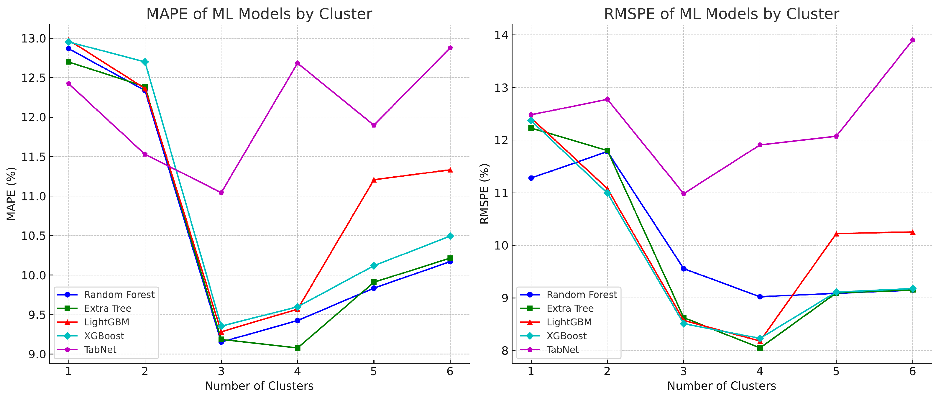
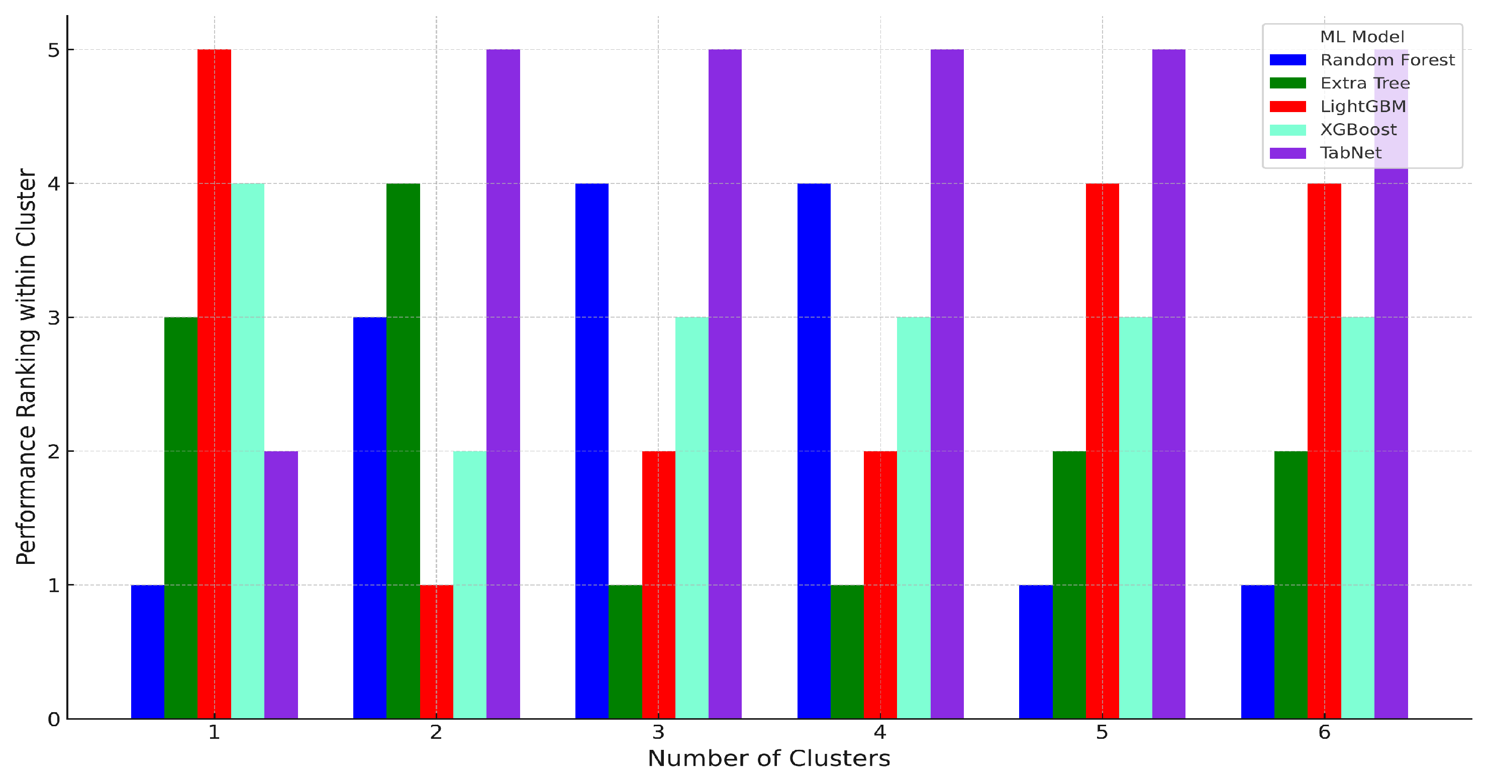
4.4. Model Results for Test Dataset

This section evaluates the accuracy of our forecasting models using the test dataset from the nested LOOCV framework. We assessed the performance of individual machine learning models and subsequently constructed and evaluated an ensemble model to enhance prediction accuracy. Our approach involved clustering the training datasets based on sales trend variables to determine the optimal number of clusters. Selecting the correct number of clusters is critical: too many clusters can dilute predictive power due to sparse data, while too few clusters may fail to capture the variability in data.

Using the nested LOOCV framework, five machine learning models were evaluated across cluster configurations ranging from one to six clusters. The inner loop was used to optimize hyperparameters and calculate the validation MAPE and RMSPE for each model, while the outer loop evaluated the final generalization performance of these models on the test dataset. Figure 4 illustrates the Test MAPE and RMSPE results for the machine learning models across different cluster configurations. The Extra Tree model, trained using four clusters, achieved the best Test MAPE and RMSPE values: 9.0779% and 8.0480%, respectively.

In contrast, the Random Forest model, which did not account for data homogeneity with its single-cluster approach, achieved MAPE and RMSPE values of 12.8683 and 11.2790, respectively. The four-cluster-based Extra Tree models demonstrated a 29% improvement in MAPE and a 28% improvement in RMSPE compared to the single-cluster Random Forest model. This significant enhancement underscores the benefits of segmenting the dataset into homogeneous clusters for better prediction accuracy. To further improve prediction accuracy, we developed an ensemble model by combining the top-performing models. We selected the “Top N” models based on their combined performance in minimizing MAPE and RMSPE across different cluster counts, as evaluated on the validation dataset. This selection process began by ranking the models according to the lowest total MAPE and RMSPE values achieved for each cluster configuration on the validation dataset. Figure 5 displays the ranking of the machine learning models based on validation performance across various cluster numbers.

The Top N ensemble model generates its final predictions by averaging the outputs of the Top N individual machine learning models. For example, in the case of a single cluster, the Top 2 ensemble model produces its final prediction by averaging the outputs of the Random Forest and TabNet models. This approach leverages the strengths of multiple high-performing models to improve prediction accuracy. To evaluate the impact of combining different numbers of models, we constructed ensemble models ranging from Top 1 to Top 5 and assessed their performance on the validation dataset. This process enabled us to determine the optimal ensemble configuration for each cluster. Finally, the generalization performance of the selected ensemble models was evaluated on the independent test dataset. Figure 6 illustrates the performance of these ensemble models, measured by their accuracy on the test dataset.

Among the ensemble configurations, the Top N ensemble model, which combines Extra Tree, LightGBM, and XGBoost models trained on data partitioned into four clusters, demonstrated the highest performance. This configuration achieved an 8% improvement in MAPE (8.3309%) and a 2% improvement in RMSPE (7.8360%) compared to the best-performing individual four-cluster Extra Tree model. Additionally, it outperformed the single-cluster Random Forest model, showing a substantial improvement of 35% in MAPE and 30% in RMSPE. These results highlight the importance of clustering, as it allows the segmentation of sales data into homogeneous groups, which enhances the interpretability of patterns and the reliability of predictions. Furthermore, the adaptability of the ensemble model across varying cluster configurations demonstrates its ability to effectively manage complex sales patterns, offering significant practical value for industries with diverse and dynamic product portfolios.

To further investigate the explanatory power of the pattern homogeneity-based prediction model, an in-depth analysis was conducted using a specific LOOCV (Leave-One-Out Cross-Validation) scenario. In this scenario, product $p=1$ was designated as the test dataset, while products $p=2$ to $p=79$ were used for training. Clustering configurations optimized for the number of clusters revealed that the four-cluster setup consistently delivered the best performance. To analyze the characteristics of trend-related variables within each cluster, the median values of these variables were derived, as depicted in Figure 7. This approach highlights the distinct behavior of each cluster, offering a clear segmentation of life cycle stages and their respective sales dynamics.

Cluster 1, characterized by a high median $x_6$ value (0.6995), represents products in the decline phase of the life cycle, where low values for $x_7$, $x_8$, $x_9$, and $x_{10}$ reflect minimal week-to-week changes and a stable but declining sales trend. Cluster 2, with a moderate median $x_6$ value (0.1980), aligns with the maturity phase, showing stable sales levels with low-to-moderate fluctuations in $x_7$ and $x_8$, and their moving averages ($x_9$ and $x_{10}$), indicative of minimal growth but consistent demand. Cluster 3, identified by a low $x_6$ value (0.0243), represents the growth phase, where moderate-to-high values for $x_7$ and $x_8$, along with their moving averages, reflect steady week-over-week sales growth and increasing market adoption. Finally, cluster 4, with the lowest $x_6$ value (0.0132), corresponds to the introduction and early growth phases, characterized by high values for $x_7$ and $x_8$ and significant moving averages ($x_9$ and $x_{10}$), indicating sharp increases in sales typical of new product launches and rapid early adoption. These clusters provide a structured framework for understanding product sales trajectories over time, aligning with the classic four stages of the product life cycle: introduction, growth, maturity, and decline [64].

Additionally,

Table 3. Distribution of dataset based on clusters.

Dataset	Cluster 1	Cluster 2	Cluster 3	Cluster 4
Training	3380	3700	1194	1669
Test	30	17	14	8

summarizes the distribution of training and test datasets across the four clusters, which correspond to distinct stages of the product life cycle. During the final model evaluation stage, the dataset is divided into training and test datasets, where the test set is reserved exclusively for assessing generalization performance. Approximately 70% of the data resides in clusters 1 and 2, which are associated with the maturity and decline phases. These phases are characterized by stable or decreasing sales trends, reflecting the prolonged nature of these stages in the electronics industry. In contrast, clusters 3 and 4, which represent the growth and introduction phases, account for a smaller proportion of the dataset. This is consistent with industry patterns, where the introduction and growth phases tend to be brief but exhibit rapid changes in sales dynamics [65].

The data distribution across clusters highlights the diversity of product life cycle stages and their unique sales behaviors. Products in cluster 1 exhibit steady declines in sales, typical of the decline phase, while products in cluster 2 maintain stable but non-growing sales, characteristic of the maturity phase. Cluster 3 captures products in the growth phase, where sales increase steadily over time, and cluster 4 represents the introduction phase, marked by rapid sales growth immediately following a product’s launch. This segmentation provides valuable insights into how sales patterns evolve across life cycle stages, enabling more accurate forecasting and targeted business strategies.

5. Conclusions

Accurately predicting the sales of new products is critical in competitive markets where profitability and operational efficiency depend on reliable forecasts. This study presents a novel forecasting framework that enhances prediction accuracy and adaptability by clustering sales data into homogeneous groups and employing tailored ensemble models for each cluster. Unlike traditional methods that rely on product-specific attributes, our approach focuses on identifying sales trends, making it particularly effective for products with unique or evolving characteristics.

The proposed framework was rigorously evaluated using a nested LOOCV approach on Korean smartphone sales data. The four-cluster Extra Tree model achieved a MAPE of 9.0779% and an RMSPE of 8.0480%, significantly outperforming a single-cluster Random Forest model by 29% in MAPE and 28% in RMSPE. Further improvements were achieved by combining top-performing models, such as Extra Tree, LightGBM, and XGBoost, in an ensemble. The ensemble model reduced MAPE to 8.3309% and RMSPE to 7.8360%, representing an 8% improvement in MAPE and a 2% improvement in RMSPE compared to the best individual model. These findings underscore the critical role of clustering to enhance data homogeneity and the complementary strengths of ensemble modeling in improving forecasting accuracy.

This study offers two primary contributions. First, it addresses the limitations of methods reliant on product attributes by introducing a clustering approach that segments sales data based on sales trends, enabling forecasts that do not depend on specific product features. Second, it demonstrates the effectiveness of integrating clustering with ensemble modeling to deliver robust and generalizable forecasts across various product life cycle stages.

From a business perspective, the proposed methodology provides actionable insights for strategic decision-making. By aligning forecasts with the product life cycle, companies can optimize inventory management, reduce risks of overstocking or stockouts, and allocate resources more effectively. Moreover, the ability to accurately predict sales for new products allows firms to innovate with greater confidence, reducing uncertainties in product launches. The segmentation of products into clusters representing distinct life cycle stages also enables targeted strategies, such as prioritizing growth-phase products or managing declining products more efficiently.

While the proposed framework demonstrates strong potential, it is not without limitations. The methodology depends on historical sales data and exogenous factors, such as Google Trends, which provide valuable insights into consumer behavior and emerging trends. However, even with the inclusion of Google Trends data, the framework may not fully account for sudden market shifts or unforeseen exogenous factors, such as macroeconomic changes, competitor actions, or changes in consumer sentiment driven by unexpected events. To address these limitations, future research could incorporate additional exogenous data sources and refine the methodology to further enhance the robustness and adaptability of the proposed framework in dynamic and volatile market environments. Moreover, extending the framework to various domains through additional research could contribute to the development of a more generalizable and universally applicable methodology.

References

- Cucculelli, M.; Peruzzi, V. Innovation over the Industry Life-Cycle. Does Ownership Matter? Res. Policy 2020, 49, 103878. [Google Scholar] [CrossRef]
- Baardman, L.; Levin, I.; Perakis, G.; Singhvi, D. Leveraging Comparables for New Product Sales Forecasting. Prod. Oper. Manag. 2018, 27, 2340–2343. [Google Scholar] [CrossRef]
- Kourentzes, N.; Trapero, J.R.; Barrow, D.K. Optimising Forecasting Models for Inventory Planning. Int. J. Prod. Econ. 2020, 225, 107597. [Google Scholar] [CrossRef]
- Huang, T.; Fildes, R.; Soopramanien, D. Forecasting retailer product sales in the presence of structural change. Eur. J. Oper. Res. 2019, 279, 459–470. [Google Scholar] [CrossRef]
- Feiler, D.; Tong, J.D. From Noise to Bias: Overconfidence in New Product Forecasting. Manag. Sci. 2021, 68, 4685–4702. [Google Scholar] [CrossRef]
- Hwang, S.; Yoon, G.; Baek, E.; Jeon, B.K. A Sales Forecasting Model for New-Released and Short-Term Product: A Case Study of Mobile Phones. Electronics 2023, 12, 3256. [Google Scholar] [CrossRef]
- Chen, I.F.; Lu, C.J. Sales forecasting by combining clustering and machine-learning techniques for computer retailing. Neural Comput. Appl. 2016, 28, 2633–2647. [Google Scholar] [CrossRef]
- Lo, J.E.; Kang, E.Y.C.; Chen, Y.N.; Hsieh, Y.T.; Wang, N.K.; Chen, T.C.; Chen, K.J.; Wu, W.C.; Hwang, Y.S.; Lo, F.S.; et al. Data Homogeneity Effect in Deep Learning-Based Prediction of Type 1 Diabetic Retinopathy. J. Diabetes Res. 2021, 2021, 1–9. [Google Scholar] [CrossRef]
- Fenza, G.; Gallo, M.; Loia, V.; Orciuoli, F.; Herrera-Viedma, E. Data set quality in Machine Learning: Consistency measure based on Group Decision Making. Appl. Soft Comput. 2021, 106, 107366. [Google Scholar] [CrossRef]
- Abuassba, A.O.M.; Zhang, D.; Luo, X.; Shaheryar, A.; Ali, H. Improving Classification Performance through an Advanced Ensemble Based Heterogeneous Extreme Learning Machines. Comput. Intell. Neurosci. 2017, 2017, 3405463. [Google Scholar] [CrossRef] [PubMed]
- Van Belle, J.; Guns, T.; Verbeke, W. Using shared sell-through data to forecast wholesaler demand in multi-echelon supply chains. Eur. J. Oper. Res. 2021, 288, 466–479. [Google Scholar] [CrossRef]
- Shwartz-Ziv, R.; Armon, A. Tabular Data: Deep Learning Is Not All You Need. Inf. Fusion 2022, 81, 84–90. [Google Scholar] [CrossRef]
- Grinsztajn, L.; Oyallon, E.; Varoquaux, G. Why Do Tree-Based Models Still Outperform Deep Learning on Typical Tabular Data? In Advances in Neural Information Processing Systems; Koyejo, S., Mohamed, S., Agarwal, A., Belgrave, D., Cho, K., Oh, A., Eds.; Curran Associates, Inc.: Nice, France, 2022; Volume 35, pp. 507–520. [Google Scholar]
- Matloob, F.; Ghazal, T.M.; Taleb, N.; Aftab, S.; Ahmad, M.; Khan, M.A. Software Defect Prediction Using Ensemble Learning: A Systematic Literature Review. IEEE Access 2021, 9, 98754–98771. [Google Scholar] [CrossRef]
- Uddin, S.; Lu, H. Confirming the statistically significant superiority of tree-based machine learning algorithms over their counterparts for tabular data. PLoS ONE 2024, 19, e0301541. [Google Scholar] [CrossRef] [PubMed]
- Cao, J.; Kwong, S.; Wang, R.; Li, X.; Li, K.; Kong, X. Class-specific soft voting based multiple extreme learning machines ensemble. Neurocomputing 2015, 149, 275–284. [Google Scholar] [CrossRef]
- Khamparia, A.; Singh, A.; Anand, D.; Gupta, D.; Khanna, A.; Arun Kumar, N.; Tan, J. A novel deep learning-based multi-model ensemble method for the prediction of neuromuscular disorders. Neural Comput. Appl. 2018, 32, 11083–11095. [Google Scholar] [CrossRef]
- Lee, H.; Kim, S.G.; Park, H.w.; Kang, P. Pre-launch new product demand forecasting using the Bass model: A statistical and machine learning-based approach. Technol. Forecast. Soc. Change 2014, 86, 49–64. [Google Scholar] [CrossRef]
- Tanaka, K. A sales forecasting model for new-released and nonlinear sales trend products. Expert Syst. Appl. 2010, 37, 7387–7393. [Google Scholar] [CrossRef]
- Elalem, Y.K.; Maier, S.; Seifert, R.W. A machine learning-based framework for forecasting sales of new products with short life cycles using deep neural networks. Int. J. Forecast. 2022, 39, 1874–1894. [Google Scholar] [CrossRef]
- van Steenbergen, R.; Mes, M. Forecasting demand profiles of new products. Decis. Support Syst. 2020, 139, 113401. [Google Scholar] [CrossRef]
- Yin, P.; Dou, G.; Lin, X.; Liu, L. A hybrid method for forecasting new product sales based on fuzzy clustering and deep learning. Kybernetes 2020, 49, 3099–3118. [Google Scholar] [CrossRef]
- Ekambaram, V.; Manglik, K.; Mukherjee, S.; Sajja, S.S.K.; Dwivedi, S.; Raykar, V. Attention Based Multi-Modal New Product Sales Time-series Forecasting. In Proceedings of the 26th ACM SIGKDD International Conference on Knowledge Discovery & Data Mining, Virtual, 23–27 August 2020; pp. 3110–3118. [Google Scholar] [CrossRef]
- Abubaker, F.; Ala’Khalifeh. Sales’ Forecasting Based on Big Data and Machine Learning Analysis. In Proceedings of the 2023 9th International Conference on Control, Decision and Information Technologies (CoDIT), Rome, Italy, 3–6 July 2023; pp. 804–808. [Google Scholar] [CrossRef]
- Smirnov, P.S.; Sudakov, V.A. Forecasting New Product Demand Using Machine Learning. J. Phys. Conf. Ser. 2021, 1925, 012033. [Google Scholar] [CrossRef]
- Afrin, K.; Nepal, B.; Monplaisir, L. A Data-Driven Framework to New Product Demand Prediction: Integrating Product Differentiation and Transfer Learning Approach. Expert Syst. Appl. 2018, 108, 246–257. [Google Scholar] [CrossRef]
- Anitha, S.; Neelakandan, R. A Demand Forecasting Model Leveraging Machine Learning to Decode Customer Preferences for New Fashion Products. Complexity 2024, 2024, 8425058. [Google Scholar] [CrossRef]
- Xu, Q.; Sharma, V. Ensemble Sales Forecasting Study in Semiconductor Industry. In Advances in Data Mining. Applications and Theoretical Aspects, Proceedings of the 17th Industrial Conference (ICDM 2017), New York, NY, USA, 12–13 July 2017; Lecture Notes in Computer Science; Perner, P., Ed.; Springer: Cham, Switzerland, 2017; Volume 10357, pp. 31–44. [Google Scholar] [CrossRef]
- Yuan, F.C.; Lee, C.H. Intelligent Sales Volume Forecasting Using Google Search Engine Data. Soft Comput. 2020, 24, 2033–2047. [Google Scholar] [CrossRef]
- Wolters, J.; Huchzermeier, A. Joint In-Season and Out-of-Season Promotion Demand Forecasting in a Retail Environment. J. Retail. 2021, 97, 73–87. [Google Scholar] [CrossRef]
- Van Donselaar, K.H.; Peters, J.; de Jong, A.; Broekmeulen, R.A.C.M. Analysis and Forecasting of Demand During Promotions for Perishable Items. Int. J. Prod. Econ. 2016, 172, 65–75. [Google Scholar] [CrossRef]
- Huber, J.; Gossmann, A.; Stuckenschmidt, H. Cluster-Based Hierarchical Demand Forecasting for Perishable Goods. Expert Syst. Appl. 2017, 77, 138–150. [Google Scholar] [CrossRef]
- Sohrabpour, V.; Oghazi, P.; Toorajipour, R.; Nazarpour, A. Export sales forecasting using artificial intelligence. Technol. Forecast. Soc. Change 2020, 163, 120480. [Google Scholar] [CrossRef]
- Chen, T.; Yin, H.; Chen, H.; Wang, H.; Zhou, X.; Li, X. Online sales prediction via trend alignment-based multitask recurrent neural networks. Knowl. Inf. Syst. 2019, 62, 2139–2167. [Google Scholar] [CrossRef]
- Bi, X.; Adomavicius, G.; Li, W.; Qu, A. Improving Sales Forecasting Accuracy: A Tensor Factorization Approach with Demand Awareness. INFORMS J. Comput. 2020, 34, 1644–1660. [Google Scholar] [CrossRef]
- Boone, T.; Ganeshan, R.; Hicks, R.L.; Sanders, N.R. Can Google Trends Improve Your Sales Forecast? Prod. Oper. Manag. 2018, 27, 1770–1774. [Google Scholar] [CrossRef]
- Skenderi, G.; Joppi, C.; Denitto, M.; Cristani, M. Well Googled Is Half Done: Multimodal Forecasting of New Fashion Product Sales with Image-Based Google Trends. J. Forecast. 2024, 43, 1982–1997. [Google Scholar] [CrossRef]
- Xiao-ping, X. More effective algorithm for K-means clustering. Comput. Eng. Des. 2008, 29, 378–380. [Google Scholar]
- Kao, Y.; Zahara, E.; Kao, I. A hybridized approach to data clustering. Expert Syst. Appl. 2008, 34, 1754–1762. [Google Scholar] [CrossRef]
- Xie, Y.; Peng, M. Forest fire forecasting using ensemble learning approaches. Neural Comput. Appl. 2019, 31, 4541–4550. [Google Scholar] [CrossRef]
- Liaw, A.; Wiener, M. Classification and Regression by randomForest. R News 2002, 2, 18–22. [Google Scholar]
- Strobl, C.; Boulesteix, A.L.; Kneib, T.; Augustin, T.; Zeileis, A. Conditional variable importance for random forests. BMC Bioinform. 2008, 9, 307. [Google Scholar] [CrossRef]
- Geurts, P.; Ernst, D.; Wehenkel, L. Extremely randomized trees. Mach. Learn. 2006, 63, 3–42. [Google Scholar] [CrossRef]
- Ke, G.; Meng, Q.; Finley, T.; Wang, T.; Chen, W.; Ma, W.; Ye, Q.; Liu, T.Y. LightGBM: A Highly Efficient Gradient Boosting Decision Tree. In Advances in Neural Information Processing Systems; Guyon, I., Luxburg, U.V., Bengio, S., Wallach, H., Fergus, R., Vishwanathan, S., Garnett, R., Eds.; Curran Associates, Inc.: Nice, France, 2017; Volume 30. [Google Scholar]
- Chen, T.; Guestrin, C. XGBoost: A Scalable Tree Boosting System. In Proceedings of the 22nd ACM SIGKDD International Conference on Knowledge Discovery and Data Mining, San Francisco, CA, USA, 13–17 August 2016; pp. 785–794. [Google Scholar] [CrossRef]
- Arik, S.Ö.; Pfister, T. TabNet: Attentive Interpretable Tabular Learning. In Proceedings of the AAAI Conference on Artificial Intelligence, Virtually, 2–9 February 2021. [Google Scholar] [CrossRef]
- Ambarwari, A.; Jafar Adrian, Q.; Herdiyeni, Y. Analysis of the Effect of Data Scaling on the Performance of the Machine Learning Algorithm for Plant Identification. J. Resti (Rekayasa Sist. Dan Teknol. Inf.) 2020, 4, 117–122. [Google Scholar] [CrossRef]
- de Amorim, L.B.V.; Cavalcanti, G.D.C.; Cruz, R.M.O. Meta-Scaler: A Meta-Learning Framework for the Selection of Scaling Techniques. IEEE Trans. Neural Netw. Learn. Syst. 2024, Early Access. [Google Scholar] [CrossRef]
- Varma, S.; Simon, R. Nested cross-validation when selecting classifiers is overzealous for most practical applications. Expert Syst. Appl. 2021, 184, 115664. [Google Scholar] [CrossRef]
- Wong, T.T. Performance evaluation of classification algorithms by k-fold and leave-one-out cross validation. Pattern Recognit. 2015, 48, 2839–2846. [Google Scholar] [CrossRef]
- Shao, Z.; Er, M.J. Efficient Leave-One-Out Cross-Validation-based Regularized Extreme Learning Machine. Neurocomputing 2016, 194, 260–270. [Google Scholar] [CrossRef]
- Hadavandi, E.; Shavandi, H.; Ghanbari, A. An improved sales forecasting approach by the integration of genetic fuzzy systems and data clustering: Case study of printed circuit board. Expert Syst. Appl. 2011, 38, 9392–9399. [Google Scholar] [CrossRef]
- Panarese, A.; Settanni, G.; Vitti, V.; Galiano, A. Developing and Preliminary Testing of a Machine Learning-Based Platform for Sales Forecasting Using a Gradient Boosting Approach. Appl. Sci. 2022, 12, 11054. [Google Scholar] [CrossRef]
- Chai, T.; Draxler, R.R. Root mean square error (RMSE) or mean absolute error (MAE)? – Arguments against avoiding RMSE in the literature. Geosci. Model Dev. 2014, 7, 1247–1250. [Google Scholar] [CrossRef]
- Bashir, N.; Mir, A.A.; Daud, A.; Rafique, M.; Bukhari, A. Time Series Reconstruction With Feature-Driven Imputation: A Comparison of Base Learning Algorithms. IEEE Access 2024, 12, 85511–85530. [Google Scholar] [CrossRef]
- Bergstra, J.; Bardenet, R.; Bengio, Y.; Kégl, B. Random Search for Hyper-Parameter Optimization. J. Mach. Learn. Res. 2012, 13, 281–305. [Google Scholar]
- Abbas, F.; Zhang, F.; Ismail, M.; Khan, G.; Iqbal, J.; Alrefaei, A.; Albeshr, M. Optimizing Machine Learning Algorithms for Landslide Susceptibility Mapping Along the Karakoram Highway, Gilgit Baltistan, Pakistan: A Comparative Study of Baseline, Bayesian, and Metaheuristic Hyperparameter Optimization Techniques. Sensors 2023, 23, 6843. [Google Scholar] [CrossRef] [PubMed]
- Probst, P.; Wright, M.N.; Boulesteix, A. Hyperparameters and tuning strategies for random forest. Wiley Interdiscip. Rev. Data Min. Knowl. Discov. 2018, 9, e1301. [Google Scholar] [CrossRef]
- Hancock, J.T.; Khoshgoftaar, T. Optimizing Ensemble Trees for Big Data Healthcare Fraud Detection. In Proceedings of the 2022 IEEE 23rd International Conference on Information Reuse and Integration for Data Science (IRI), San Diego, CA, USA, 9–11 August 2022; pp. 243–249. [Google Scholar] [CrossRef]
- Ryu, S.E.; Shin, D.H.; Chung, K. Prediction Model of Dementia Risk Based on XGBoost Using Derived Variable Extraction and Hyper Parameter Optimization. IEEE Access 2020, 8, 177708–177720. [Google Scholar] [CrossRef]
- Bentéjac, C.; Csörgo, A.; Martínez-Muñoz, G. A comparative analysis of gradient boosting algorithms. Artif. Intell. Rev. 2020, 54, 1937–1967. [Google Scholar] [CrossRef]
- Zhang, L.; Suganthan, P. Visual Tracking With Convolutional Random Vector Functional Link Network. IEEE Trans. Cybern. 2017, 47, 3243–3253. [Google Scholar] [CrossRef] [PubMed]
- Osawa, K.; Tsuji, Y.; Ueno, Y.; Naruse, A.; Foo, C.S.; Yokota, R. Scalable and Practical Natural Gradient for Large-Scale Deep Learning. IEEE Trans. Pattern Anal. Mach. Intell. 2020, 44, 404–415. [Google Scholar] [CrossRef] [PubMed]
- Thietart, R.; Vivas, R. An Empirical Investigation of Success Strategies for Businesses Along the Product Life Cycle. Manag. Sci. 1984, 30, 1405–1423. [Google Scholar] [CrossRef]
- Zhu, X.; Jiao, C.; Yuan, T. Optimal decisions on product reliability, sales and promotion under nonrenewable warranties. Reliab. Eng. Syst. Saf. 2019, 192, 106268. [Google Scholar] [CrossRef]